Feb 15, 2013 - regions which are significantly before of behind the object of interest. .... Mask Approximation, Color Segmentation and Re- gion Scoring.
Robust Image Segmentation in Low Depth Of Field Images
arXiv:1302.3900v1 [cs.CV] 15 Feb 2013
Franz Graf, Hans-Peter Kriegel, and Michael Weiler Ludwig-Maximilians-Universitaet Muenchen, Oettingenstr. 67, 80538 Munich, Germany [graf,kriegel,weiler]@dbs.ifi.lmu.de February 19, 2013
Abstract
regions which are significantly before of behind the object of interest.
In photography, low depth of field (DOF) is an important technique to emphasize the object of interest (OOI) within an image. Thus, low DOF images are widely used in the application area of macro, portrait or sports photography. When viewing a low DOF image, the viewer implicitly concentrates on the regions that are sharper regions of the image and thus segments the image into regions of interest and non regions of interest which has a major impact on the perception of the image. Thus, a robust algorithm for the fully automatic detection of the OOI in low DOF images provides valuable information for subsequent image processing and image retrieval. In this paper we propose a robust and parameterless algorithm for the fully automatic segmentation of low DOF images. We compare our method with three similar methods and show the superior robustness even though our algorithm does not require any parameters to be set by hand. The experiments are conducted on a real world data set with high and low DOF images.
Low DOF images are well known from sports, portrait or macro photography where only a specific part of the image should attract most of the users’ attention. The OOI is thereby displayed sharp while other areas like the background appears blurred, so that the viewer automatically focuses on the sharp areas of the image. When viewing a low depth of field image, the viewer implicitly segments the image into regions of interest and regions of less interest (usually background). As this implicit segmentation has major impact on the perception of the image, this information is a valuable feature for the subsequent image processing chain like an adaptive image compression [6] or image retrieval aspects such as the similarity of images which can be considerably influenced by the image’s DOF. Given for example two images displaying a person in the sharp image region in front of different, blurred backgrounds, people might judge both pictures similar even though the blurred background differs. Although this implicit segmentation is rather easy for a human viewer of the photo, it is not an easy task for a completely unsupervised algo1 Introduction rithm. This can be explained by the fact that there is In photography, low depth of field (DOF) is an im- usually not a sharp edge which divides the sharp OOI portant technique to emphasize the object of interest and blurred background. Depending on the camera’s (OOI) within an image. Low DOF images are usually setting, this transition can be very smooth so that it characterized by a certain region which is displayed is hard to distinguish where the OOI ends. With the vastly growing market of consumer very sharp like the face of a person and blurry image 1
DSLRs or even new small compact cameras like the Sony Cybershot which are explicitly being advertised with the ability for low DOF photos, the amount of low DOF photos also increased. This growing amount of low DOF images may also provide new information for established search and retrieval systems if they take the OOI into account when performing the similarity search tasks. In order to profit from the low DOF information, search engines and feature extraction algorithms need fully automatic and robust image segmentation algorithms which can separate the OOI from the rest of the image. For large search engines or image stock agencies, such algorithms should also be independent of the image domain, image size and the color depth of the image so that the algorithm performs well, no matter of the color or the toning of the photo (e.g. black-and-white, color photos, sepia photos). In this paper, we propose a robust, fully automatic and parameterless algorithm for the segmentation of low DOF images as well as an analysis of the impact of low DOF information on similarity search. The algorithm does not need any a priory knowledge like image domain or camera settings. The algorithm also provides meaningfull results even if the DOF is rather large so that the background provides significant structures. The rest of the paper is organized as follows: In Sec. 2 we review some related work and some technical background, follwed by the explanation of the algorithm in Sec. 3. In Sec. 4 we explain our experimental evaluation of the algorithm. In Sec. 5 we describe the internal parameter settings and threshold values. The impact of the DOF segmentation to image similarity is shown in Sec. 6. Afterwards we finish the paper with a conclusion and outlook in Sec. 7.
tered. Afterwards the edges are linked to form closed boundaries. These boundaries are treated with a region filling process, generating the final result. [12] presents a fully automatic segmentation algorithm using block based multiresolution wavelet transformations on gray scale images. Even though the paper lists high rates of sensitivity and specificity on the testset, the authors also name some limitations like the dependence on very low DOF, fully focused OOI, and high image resolution and quality. In [16, 15] high frequency wavelets are used to determine the segmentation of low DOF images. As stated in [9], these features have the drawback of being not too robust if used alone and thus often result in errors in both focused and defocused regions if the defocused background shows some busy textures or if the focused foreground does not have very significant textures. In [10], localized blind deconvolution is proposed to determine the focus map of an image. Yet the authors do not propose a pure image segmentation algorithm as the focus map is not a true segmentation but a measure for the amount of focus in this part of the image. Also the algorithm does not take into account any color information as it is only operating on gray scale images. The works proposed in [9, 13, 7, 8] are consecutive works for segmentation of DOF images and sequences of images [9, 13] like in movies which address a similar topic. In this paper, we were inspired by the algorithm proposed in [7] which uses morphological filtering for the segmentation. Some problems of this algorithm were given by background that showed significant structures or if a photo was taken with high ISO values. Also the algorithm showed some problems if spatially separated OOIs were shown in a single image. Another problem can be raised by the size of the structuring element used in the algorithm [7, Sec. IV]. We compare our algorithm with the work of [7], with [11] where single frames of videos are processed 2 Related work into a saliency map which is processed by morphoThe segmentation of low DOF images has gained logical filters. The resulting tri-map is then used for some interest in the research community in past error control and for the extraction of boundaries of years. In [12, 14] early approaches to segment low the focused regions. We also compare our work to the DOF images were presented. Thereby [14] is using an algorithm proposed in [18], where a fuzzy segmentaedge-based algorithm which first converts a gray-scale tion approach was proposed by first separating the image into an edge-representation which is then fil- image into regions using a mean shift. These regions 2
2.1
ffocal pla ane
apertu ure
are then characterized by color features and wavelet modulus maxima edge point densities. Finally, the region of interest and the background are separated by defuzzification on fuzzy sets generated in the previous step. Our test image dataset consists of a set of various photos and comprises several categories from high to low DOF images.
perceived sharp area
Depth of Field Fig. 1: Figure illustrating the depth of field. The size of the perceived sharp area around the focal plane denotes the DOF.
In optics, the DOF denotes the depth of the sharp area around the focal point of a lens seen from the photographer. Technically, each lens can only focus at a certain distance at a time. This distance builds the focal plane which is orthogonal to the photographers view through the lens. Precisely, only objects directly on the focal plane are absolutely sharp, while objects before or behind the focal plane are displayed unsharp. With increasing distance from the focal plane, the sharpness of the displayed object decreases. Nevertheless, there is a certain range before and behind the focal plane where objects are recognized as sharp until a blur is perceived. The depth of this region is then called the DOF. As the sharpness decreases gradually with increasing distance from the focal plane, it is hard to determine an exact range for the DOF as the limits of the sharp area are only defined by the perceived sharpness. Points in the defocused areas appear blurred to a certain degree. This is often modeled by a Gaussian kernel Gσ as in Eq. 1 where σ denotes the spread parameter which affects the strength of the blur. For a given image I, the blurred representation can then be created by a convolution Gσ ∗ I. � 2 � x + y2 1 exp − (1) Gσ (x, y) = 2πσ 2 2σ 2
2.2
Automatic segmentation of low DOF images
Automatic segmentation of images is more challenging than interactive approaches because no additional information of humans can be used to adapt parameter values for the segmentation process. However the advantages of a fully automated algorithm are obvious, if the according algorithm should be deployed to a system providing lots of images where the segmentation should be present as fast as possible. This is for example the case in search index or photo communities like Flickr or Google’s Picasa, where several thousand photos are uploaded each minute, even if not all of them are low DOF images. The requirements to a segmentation algorithm are that it should be able to handle different types (grayscale or color), orientations (landscape or portrait) and resolutions (from small to large) of images, independent of the camera settings like ISO etc. Many automatic segmentation approaches of low DOF images have some of these restrictions, as seen in [18], which only performs well on color images. Grayscale images mostly fail because the extracted color features are too few, to characterize regions and distinguish them sufficient. However, other algorithms like the one presented in [7], can only process grayscale images. In such cases, color images have to be transformed and hence their color information looses its contribution to improve segmentation quality. As shown in our experimental
The effect of DOF is mainly determined by the choice of the camera respectively its imaging sensor size, aperture and distance to the focussed object. The larger the sensor or aperture, the smaller the DOF. Increasing the distance from the camera to the focussed object will also expand the resulting DOF. Figure 1 illustrates the geometry of DOF at a symmetrical lens. 3
results in section 4, images that consist of complex defocused regions can cause poor segmentation results, because too many false positives are found. In this context, false positives describe the set of pixels that are defined as background by the underlying ground truth but classified as OOI pixel by the segmentation algorithm. In the following section, we describe our algorithm that does not suffer from one of the restrictions mentioned above. Therefore, we use a robust method for calculating the amount of sharpness of a pixel in relation to its neighbors by taking advantage of the L∗ a∗ b∗ color space, which offers a more accurate matching between numerical and visual perception differences between colors. The L∗ a∗ b∗ model was favored over the well known RGB and CM Y K color spaces, as the L∗ a∗ b∗ model is designed to approximate human vision better than the other color spaces. To accomplish the problems caused by images consisting of numerous less blurred pixel regions showing complex structures, we apply a density-based clustering algorithm to all found sharp pixels. This enables our algorithm to distinguish between sharp pixels belonging to the main focus region of the OOI (if these pixels belong to the largest found cluster) and noise pixels located in background structures.
In the second stage, called Score Clustering, all pixels with a score value above a certain threshold are clustered by using a density-based clustering algorithm. Thus, isolated sharp pixels are recognized as noise and only large clusters are processed further. The third stage named Mask Approximation generates a nearly closed plane (containing almost no holes) from the discrete points of each remaining cluster. This is achieved by computing the convex hull from all neighbors of all dense pixels. Any so-created polygon is then filled and the union of these filled regions represent the approximate mask of the main focus region. In the next two stages this approximate mask is going to be refined. Hence, the fourth stage, called Color Segmentation divides the approximate mask into regions that contain pixels with similar color in the original image. In the fifth stage named Region Scoring, a relevance value is calculated for each region. This relevance value is directly influenced by the score values of the pixels surrounding the according region. The final segmentation mask is then created by removing all regions that have a relevance value below a certain threshold.
3.1
3
Deviation Scoring
In the first step, we need to identify sharp pixels as an indication for the focused objects within the image. The well known Canny edge detector [2] is not suitable in this case because the Canny detector operates on gray scale images and not on the L∗ a∗ b∗ color space. Furthermore, the Canny operator does not aim at the detection of single edge pixels but at the robust detection of lines of edges even in partly blurred areas of the image (c.f. Fig. 3b on page 6). The HOS map used in [7] is defined as in Eq. 2
Algorithm
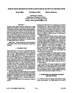
The proposed algorithm consists of the following five stages: Deviation Scoring, Score Clustering, Mask Approximation, Color Segmentation and Region Scoring. Before explaining the steps of the algorithm in detail, we first want to give a brief summary of the complete algorithm. Fig. 2 illustrates the steps of the algorithm. The first stage of the algorithm, called Deviation Scoring, identifies sharp pixel areas in the image. � � Therefore a Gaussian Blur is applied to the original m ˆ (4) (x, y) , (2) HOS (x, y) = min 255, image. The difference between the extracted edges DSF from the original image and the blurred image is then calculated. For each pixel, this difference repre- where DSF represents a down scaling factor of 100 sents a score value, with higher score values indicat- and the forth-order moment m ˆ (4) at (x, y) is given by P 4 ing sharper pixels and lower score values indicating m 1 (4) ˆ (x, y) = Nη (I (s, t) − m ˆ (x, y)) where blurred pixels. (s,t)∈η(x,y) 4
(a) Input Image
(b) Deviation Scor- (c) Score Clustering (d) Mask Approxi- (e) Color Segmenta- (f) Region Scoring ing mation tion
Fig. 2: Illustration of the five stages of our algorithm: Fig. 2a: Input image with low DOF and relatively complex background regions. Fig. 2b: Identify sharp pixels by computing the difference between the edges of the original image and the edges of the blurred version of the image. Fig. 2c: Generate clusters from pixels with a high appropriate score by a density-based clustering algorithm (for a better visual representation we colored each found cluster and surround it with its convex hull). Fig. 2d: Filling all convex hulls from all neighbors of all dense pixels. Fig. 2e: Group pixels 5into regions that contain similar colored pixels in the original image. (For a better visual representation we colored each found region in a random color). Fig. 2f: Removing all color Regions with low relevancy.
m ˆ is the sample mean and defined as in Eq. 3 m ˆ (x, y) =
1 Nη
X
I (s, t) .
(3)
(s,t)∈η(x,y)
Thereby η (x, y) is the set of neighborhood pixels with center (x, y) and is set to size 3 × 3 where Nη denotes its cardinality. Using the HOS map also has the disadvantage that it operates only on gray scale images. Additionally, the HOS map is too sensitive in case of textured background as it only produces reasonable results if the background is significantly blurred. This works for images with very low DOF, but as soon as the DOF is not very small, the HOS map detects too many sharp areas in the background (c.f. Fig. 3c). Thus, we propose the process of Deviation Scoring. Let I be the set of pixels of the processed image. For each pixel p (x, y) ∈ I, the mean color from the pixel’s r-neighborhood is calculated by r ηI(x,y) = {p (x0 , y 0 ) | |x0 − x| ≤ r ∧ |y 0 − y| ≤ r}
(a) Original image
(b) Canny Edge Detection
(c) Higher Order Statistics
(d) Deviation Scoring
with r representing the L1-distance to the pixel p(x, y). The color value of p(x, y) is represented in � the L∗ a∗ b∗ color space and denoted by L∗p , A∗p , Bp∗ . Thus, the mean neighborhood color of p(x, y) in the L∗ -band is determined by � P L∗p r LηI(x,y) =
r p∈ηI(x,y)
r ηI(x,y)
.
The values for the a∗ - and b∗ -band are denoted by r r aηI(x,y) and bηI(x,y) respectively, so that the mean r neighborhood color LabηI(x,y) of a pixel p(x, y) is de� � r r r fined by LηI(x,y) , aηI(x,y) , bηI(x,y) . According to the International Commission on Illumination CIE 1 , the color distance ∆E ∗ (u, v) between two color values u, v in the L∗ a∗ b∗ color space is calculated by using the Euclidean distance: q 2 2 2 ∆E ∗ (u, v) = (L∗u − L∗v ) + (a∗u − a∗v ) + (b∗u − b∗v ) 1 CIE: Commission http://www.cie.co.at
Internationale
de
Fig. 3: Comparison of edge detection techniques.
l’eclairage,
6
values µ ∈ [0, 255] of the edge pixels. Therefore, the score µ(x, y) for an edge pixel p (x, y) is determined by the squared neighbor difference in the images I 0 and Iσ0 at the location of the according pixel: � � �2 � µ (x, y) = min 255, ∆ηIr0 (x,y) − ∆ηIrσ0 (x,y)
(a) HSV (0, 1, 1) increased in component H.
(b) HSV (0, 0, 1) increased in component S.
Due to the limitation to µ(x, y) ≤ 255, we are treating all color changes between I 0 (x, y) and I(x, y) (c) HSV (0, 0, 0) increased in component V . equally where ∆E > 16. This can be justified by human perception, which recognizes two colors u, v Fig. 4: Visualization of the ∆E ∗ color distance within to as rather unsimilar to each other if ∆E ∗ (u, v) > 12 each component of the well known HSV color space, [3]. Thus it can be said, that a ∆E ∗ > 16 indicates with colors c0 , . . . , c9 . Where ci of the i -th square is a significant color change which is also a strong indiincreased in each of the components H (Fig. 4a), S cation for an edge. (Fig. 4b) and V (Fig. 4c) so that ∆E ∗ (ci , ci+1 ) ≈ 16. Afterwards, all edge pixels with a score value greater than the threshold Θscore are treated as canr For each p (x, y), the neighbor difference ∆η(x,y) is didates for the focused region of the image while the score values of all pixels having a score value less than then defined by Θscore are set to 0 and are thus no candidates. The � � resulting candidate set Iscore (x, y), is defined by the r ∆E ∗ LabηI(x,y) ,p following equation: r ∆ηI(x,y) = min 255 · , 255 ∆E max ( 0 µ (x, y) < Θscore Iscore (x, y) = max with ∆E being the maximum possible distance in µ (x, y) else the L∗ a∗ b∗ color space and ∆E ∗ (u, v) being the Euclidean distance of the color values u, v in the L∗ a∗ b∗ An illustration of the candidate set can be seen in space. In Fig. 4 we illustrated a color distance of Fig. 3d and Fig. 2b, where brighter pixels indicate a ∆E ∗ = 16 , by varying one of the three components large score and black pixels indicate a score less than the threshold Θscore . of a base color defined in the HSV color space . In the following, all pixels p (x, y) with a neighbor difference greater than the threshold Θscore ∈ [0, 255] 3.2 Score Clustering are called edges or edge pixels, so that the equation r > Θscore holds for each edge pixel of the In this step, clusters are generated from all points in ∆ηI(x,y) image. Even though the parameter Θscore could be Iscore in order to find compound regions of focused set freely, we recommend a value of 50 (c.f. Tab. 1) areas. Therefore, the density-based clustering algoas it showed the best result. Before calculating the rithm DBSCAN [4] is used. In contrast to the Kscore values of the edge pixels, I is convolved using Means [5], which partitions the image into convex a Gaussian kernel with a standard deviation σ = Θσ clusters, DBSCAN also supports concave structures to remove noise and generally soften the image. We which is more desirable in this case. The following 1 recommend to set the value of Θσ to 10 (c.f. Tab. 1). section gives a short outline of DBSCAN and then deThe resulting image is then denoted by I 0 . scribes how the necessary parameters ε and minP ts Afterwards, another image Iσ0 is created by con- are determined automatically and how DBSCAN is volving I 0 once again by using the same Gaussian used in our segmentation algorithm for further prokernel. I 0 and Iσ0 are then used to compute the score cessing. 7
them relatively to the size of the image andpits score distribution. Thus, ε is calculated by ε = |I| · Θε , In this stage, clusters are generated from all p ∈ Iscore with |I| denoting the total amount of pixels of the by applying DBSCAN, which is based on the two paimage represented by I and Θε ∈ [0, 1]. The second rameters ε and minP ts. The main idea of this clusparameter minP ts is determined by tering algorithm is that each point in a cluster is lo cated in a dense neighborhood of other pixels belong� � X (ε + 1)2 µ(x, y) ing to the same cluster. The area in which the neigh- minP ts = min , 1 , |I| Θdbscan bors must be located is called the ε-neighborhood of a (x,y)∈Iscore point, denoted by Nε (p), which is defined as follows: with the threshold Θdbscan set to 255. Nε (p) = {q ∈ D | dist (p, q) ≤ ε} (4) The result of the DBSCAN clustering is a cluster set C = {c1 , . . . , cn }, with each ci ∈ C representing where D is the database of points and dist (p, q) de- a subset of pixels p(x, y) ∈ I. Due to our assumption scribes the distance measure (e.g. the Euclidean dis- that small isolated sharp areas are treated as noise, tance) between two points p, q ∈ D. we define the relevant score cluster set For each point p of a cluster C there must exist a n maxC o point q ∈ C so that p is within the ε-neighborhood of Cˆ = c ∈ C | |ci | ≥ ⊆ C, 2 q and N (p) includes at least minP ts points. There3.2.1
DBSCAN
ε
fore some definitions are invoked which are described in the following. Considering ε and minP ts, a point p is called directly density-reachable from another point q, if p ∈ Nε (p) and p is a so-called core-point. A point p defined as a core-point if |Nε (p)| ≥ M inP ts holds. If there exists a chain of n points p1 , . . . , pn , such that pi+1 is directly density-reachable from pi , then pn is called density-reachable from p1 . Two points p and q are density-connected if there is a point o from which p and q are both density reachable, considering ε and minP ts. Now, a cluster can be defined as a non-empty subset of the Database D, so that for each p and q, the following two conditions hold:
with maxC = max {|c1 | , . . . , |cn |} being the amount of pixels of the largest cluster. An illustration of this step can be seen in Fig. 2c on page 5 where different clusters are painted in different colors.
3.3
Mask Approximation
ˆ as defined in section The relevant score cluster set C, 3.2, is already a good reference point of the OOI’s location and distribution. In general however, there exists no single contiguous area, but several individual regions of interest representing the focused objects. This stage of the algorithm connects all clusters c ∈ Cˆ to a contiguous area which represents an approximate binary mask of the OOI. This is achieved • ∀p, q : if p ∈ C and q is density-reachable from through the two steps Convex Hull Linking and Morp, then q ∈ C phological Filtering, that will be described in more detail below. • ∀p, q ∈ C : p is density-connected to q
Points that do not belong to any cluster are treated 3.3.1 Convex Hull Linking as noise = {p ∈ D | ∀i : p ∈ / Ci }, where i = 1, . . . , k In the convex hull linking step we first generate and C1 , . . . , Ck are the found clusters in D. the convex hull for all points in the ε-neighborhood NEps (p) of each core point p of the cluster set. 3.2.2 Determination of Parameters Let K = {k1 , . . . , kj } be the set of all core points To provide highest flexibility with respect to the dif- from the score clusters in Cˆ and let convex(P ) be ferent occurrences of the focused area, we do not ap- the convex hull of a point set P . Then we can ply absolute values for ε and minP ts, but compute define the set of convex hull polygons by H = 8
{convex(Neps (k1 )), . . . , convex(Neps (kj ))} which is used to generate a contiguous area. Therefore each p (u, v) ∈ I is checked, if it is located within one of the convex hull polygons of H. If that is the case, we mark this pixel with 1, otherwise with 0. The binary approximation mask Iapp is then given by ( 1 if ∃Hi : p(x, y) ∈ Hi Iapp (x, y) = . 0 otherwise
dilation. The geodesic erosion ε(∞) and dilation δ (∞) of infinite size, called reconstruction by erosion ϕ(rec) and reconstruction by dilation γ (rec) , is then defined as follows ϕ(rec) (I, I 0 ) = ε(∞) (I, I 0 ) = ε(1) ◦ . . . ◦ ε(1) (I, I 0 ) γ (rec) (I, I 0 ) = δ (∞) (I, I 0 ) = δ (1) ◦ . . . ◦ δ (1) (I, I 0 ) Note that ϕ(rec) (·, ·) and γ (rec) (·, ·) converge and achieve stability after a certain number of iterations. Thus it is assured that these functions do not need to be executed indefinitely and so the application is guaranteed to terminate.
Afterwards we apply the morphological filter operations closing and dilation by reconstruction to Iapp for smoothing and closing small holes. 3.3.2
Morphological Filtering
3.3.3
Morphological filters are based on the two primary operations dilation δH (I) and erosion εH (I) where H (i, j) ∈ {0, 1} denoting the structuring element. For a binary image I, δH (I) and εH (I) are defined as in the following equations:
Application
In our approach, we primarily apply a morphological closing operation ϕH (Iapp ) = εH (δH (Iapp )) to the approximate mask. The dimension of the structuring element H therefore is discussed later. Afterwards we use ϕrec (Iapp , δH 0 (Iapp )) to close holes in the approximate mask Iapp . The dimension of the structuring element H is h × h, where h is calculated relatively to the total p pixel count |Iapp | of the image Iapp , so that h = |Iapp | · Θrec , with Θrec ∈ [0, 1]. After this morphological processing, the approximate mask Iapp covers the OOI quite well (c.f. Fig. 2d on page 5). In general however, it includes boundary regions that exceed the borders of the OOI and tend to surround it with a thick border. The following two stages of our algorithm refine the mask by erasing the surrounding border regions.
δH (I) = {(s, t) = (u + i, v + j) | (s, t) ∈ I, (i, j) ∈ H} εH (I) = {(s, t) | (s + i, t + j) ∈ I, ∀ (i, j) ∈ H} The operation morphological closing ϕH , is a composition from the two primary operations, so that ϕH (I) = εH (δH (I)). Thus, the input image I is initially dilated and subsequently eroded, both times with the same structuring element H. In order to define the following operation dilation by reconstruction, some more definitions are required. At first, the primary operations δH (I) and εH (I) are extended to the basic geodesic dilation δ (1) (I, I 0 ) and basic geodesic erosion ε(1) (I, I 0 ) of size one as in the following equations.
3.4
Color Segmentation
In this stage, the pixels from the approximate mask Iapp are divided into groups, so that each group contains pixels that correspond to similar colors in I. ε(1) (I, I 0 ) (u, v) = max {εH (I) (u, v) , I 0 (u, v)} Therefore we process each p (u, v) ∈ Iapp and iteraNote that these basic geodesic operations need an tively include all its neighbors n for which the followadditional Image I 0 , which is called marker, where ing conditions hold: n o the input image I is called mask. Thus, the result of 1 n ∈ (s, t) ∈ η | I (s, t) = I (u, v) = 1 app app Iapp (u,v) a geodesic erosion at position (u, v) is the maximum value of the erosion εH of mask I and the value of the marker image I 0 (u, v) and vice versa for the geodesic ∧ ∆E ∗ (p, n) < Θdist . (5) δ (1) (I, I 0 ) (u, v) = min {δH (I) (u, v) , I 0 (u, v)}
9
The threshold Θdist ∈ [0, 100] is an internal parameter, which specifies the maximum distance between two color values u, v in the L∗ a∗ b∗ color space. Therefore a method expand(x, y, R) is called for each p (x, y) ∈ {(x, y) ∈ Iapp | Iapp (x, y) = 1}, which is not yet marked as visited. R = {(x, y)} here defines a new color region formed by the point p1 (x, y). The method expand(x, y, R) then proceeds as follows: For all neighbors p2 (x, y) of p(x, y) fulfilling Eq. 5 on the preceding page we add p2 to R and mark p (u, v) as visited. Then expand (u, v, R) is called recursively. The resulting set of regions is called Rcolor .
3.5
Region Scoring
eliminate all regions r with a mask relevance value which is too low. The calculation of M Rr is executed iteratively: Let M Rri denote the value M Rr of a region r during the i-th iteration. One iteration cycle computes the corresponding µ for each region r and deletes r from the approximate mask Iapp if M Rri ≤ Θrel . The precise assignment of Θrel and its impact on segmentation quality is discussed later. Once a region r satisfies M Rri ≤ Θrel at iteration i, it will be erased from Iapp , so that ∀ (x, y) ∈ r : Iapp (x, y) = 0. The calculation of M Rri continues for i = 1, . . . m iterations and terminates as soon as there are no more regions to delete. This is the case, as soon as M Rri = M Rri−1 such that ∃m ≥ 1 | ∀r ∈ Rcolor : M Rri = M Rri−1 .
In this step, a relevance value µ is calculated for each region r ∈ Rcolor . The more a region is surrounded by areas with a large score µ, the larger the relevancy value gets. Low relevant regions are removed after- 4 Experimental Results wards which causes an update of µ in the neighboring regions and thus possibly triggers another deletion if The proposed algorithm is designed to be parameterthe relevance of an updated region is not high enough less and thus applicable to different types of images after the according update. without having to adjust parameter values by hand. The quality of the resulting segmentation only de3.5.1 Boundary Overlap pends on the size and resolution of the input image. The boundary overlap BOrR of a region r is a measure In this section we discuss the quality measure for the for the adjacency of r to the approximate mask Iapp comparison of different segmentation algorithms and we show key features, such as the amount of depth and is defined as of field, that affects difficulties in segmentation. FurBOrR = |{(u, v) ∈ Br | ∃r0 ∈ R : (u, v) ∈ r0 }| , ther more, we demonstrate that images with higher where Br is the difference of r to its dilation. The resolution generally lead to be better segmentation mask boundary overlap M BOr of r is then defined results in contrast to the reference algorithms, which Rcolor loose accuracy with growing size of the processed imr . M BOr specifies the ratio of age. as M BOr = BO|B r| the number of outline points located in other regions In 4.3 we describe the internal parameters and to the number of all outline points of r. ˆ threshold values that we determined during our deBO C The score boundary overlap SBOr = |Brr| of r is a velopment and testing phases and show their impact measure for the adjacency of r to the corresponding on the quality of the segmentation result and the perscore values µ. A large SBOr indicates, that r has a formance. neighborhood with large corresponding score values µ. 3.5.2
4.1
Mask Relevance
The mask relevance for a given region r can then be defined as M Rr = SBOr · M BOr . Afterwards, we
Quality measure
To determine the quality of a segmentation mask I we use the spatial distortion d0 (I, Ir ) as proposed in 10
Table 1: Parameters used in the algorithm.
[7]: P d0 (I, Ir ) =
I (x, y) ⊗ Ir (x, y)
(x,y)
P
Ir (x, y)
,
(x,y)
where ⊗ is the binary XOR operation and Ir is the manually generated reference mask that represents the ground truth. The spatial distortion denotes the occurred errors, false negatives and false positives, in relation to the size of the reference mask Ir , which is equivalent to the sum of all true positives and false negatives. Notice that d0 can grow larger than 1 if more pixels are misclassified than the number of foreground pixels in total. Let ï¿œ be a blank mask so that ï¿œ(x, y)=0 for each pixel p (x, y). The number of false negatives is now equal to the foreground mask pixel in I because no pixel in ï¿œ is defined as forground. For each image I, the spatial distortion d (ï¿œ, I) = 1 . Thus we limit d0 to d ∈ [0, 1], so that d (I, Ir ) = min {1, d0 (I, Ir )} .
4.2
Dataset
All experiments were conducted on a diverse dataset of 65 images downloaded from Flickr and created by our own. The images are from different categories with strong variations in the amount of depth of field, as well as in the fuzziness of the background. Also the selection of the images does not focus on certain sceneries, topics or coloring schemes in order to avoid overfitting to certain types of images. In our experiments, we compare the spatial distortion of the proposed algorithm with re-implementations of the works presented in [7], [11] and [18]. The parameters for all algorithms were optimized to achieve the best average spatial distortion over the complete test set.
4.3
Comparison
A major contribution of this algorithm is that none of the parameters introduced in the previous section needs to be hand tuned for an image as all parameters are either independent of the image or determined fully automatically. An overview of the implicit parameters and their default values can be seen in Table 1. 11
Parameter Θscore Θ� Θσ Θdist Θrec Θrel
Value 50 1 40 1 10
25 1 3 2 3
Description Score µ threshold of Iscore Spatial radius of DBSCAN Gaussian blur radius Color similarity distance Relative size of reconstruction Minimum value of relevant regions
To calculate the score image Iscore we use a Gaus1 sian blur with standard deviation of Θσ = 10 . Iscore is then scaled to fit in 400 × 400 pixel to improve the processing speed of the subsequent steps without major impact to accuracy. We set Θscore = 50 so that a score µ must exceed 50 to be processed by the density-based clustering algorithmp DBSCAN that uses a neighborhood distance ε = Θ� |I|, where |I| is the total pixel count of image I and minP ts is calculated in dependence of ε, as described in Sec. 3.2.2. To smooth the approximate mask we use the morphological operation reconstruction p by dilation γ rec with a structuring element H of size |Iapprox | · Θrec where Θrec = 31 . Further we set the maximum distance threshold of similar color values in the L∗ a∗ b∗ color space to Θdist = 25. The refinement of the approximate mask removes all regions with a mask relevance value less than Θrel = 32 . Fig. 6 compares the performance of the reference algorithms with our proposed method. It can be seen that even though the computation time of the proposed algorithm is greater than two of the three reference algorithms, it outperforms the reference algorithms in terms of spatial distortion in all cases. Also, our algorithm has an average spatial distortion error of 0.21 over the complete test set which is less than half compared to the best competing algorithm with an average of 0.51 for the morphological segmentation with region merging [7]. Our algorithm also provides the lowest minimum error of 0.01 in contrast to 0.02 for the fuzzy segmentation algorithm [18]. It should also be noted that in contrast to the reference algorithms, the proposed algorithm shows improved accuracy with larger images whereas the competitors loose accuracy with growing size of the im-
Errror
Table 2: Spatial distortion and run time of the rate segmentation. Images with smaller DOF, homoproposed algorithm compared to the reference algo- geneous defocused regions and variant colors tend to rithms. produce much better segmentation results than images with high DOF, complex defocused regions and Proposed [7] [18] [11] plain colors. The first type of images is commonly Minimum 0.01 0.05 0.02 0.07 used by most of the competitors’ publications to enMedian 0.10 0.48 0.93 1 sure a high segmentation quality of the presented alAverage 0.21 0.51 0.84 0.81 gorithm. Figure 7 shows the minor segmentation difStd.Dev. 0.21 0.26 0.25 0.31 ferences of a small DOF image. A much more chalTime 28s 9s 54.2s 2.7s lenging task is the segmentation of images with complex background as shown in Fig. 8. Thereby our pro1,00 posed algorithm achieves a good segmentation result 0,90 , with a spatial distortion of 0.21 (c.f. Fig. 8b), where 0,80 the other segmentation algorithms [18], [7] and [11] 0 70 0,70 fail with spatial distortion values of each larger than 0,60 0.69 (c.f. Fig. 8c, 8d and 8e). 0 50 0,50 0,40
4.5
0,30 0,20 0,10 0,00 1
11
21
31 41 Image No.
51
61
Fig. 5: Spatial distortion error values of the segmentation with our proposed algorithm for each of the 65 dataset images. age. The minimum, median, average and standard deviation of the spatial distortion error are listed in Tab. 2. In Fig. 5 we illustrate all spatial distortion error values for each segmented image in the dataset.
4.4
Image Types
For each image we can define key features as in table 3. All these features affect the difficulty for an a accuTable 3: Key features of an Image amount of DOF small high
defocused regions homogeneous complex
color plain variant 12
Size of input image
One of the most influential variables on segmentation quality is the resolution of the input image. A comparatively high resolution is needed for a proper segmentation, if for example an image has just a slightly defocused background and thus shows significant texture. Thus we designed the algorithm to be able to handle a large scope of resolutions properly without loss of quality. By using the image of Fig. 8a as input, a spatial distortion value of 0.65 can already be achieved at the relatively small resolution of 200 × 300 pixels. For this particular image, a resolution of 240 × 350 is needed to lower the spatial distortion to 0.42. Fig. 9 shows the diversification of average and standard deviation of the spatial distortion depending on the increase of image size. Because the orientation (portrait or landscape) and aspect ratio (2:3, 4:3, etc.) of the images in our test set varies, we rescale each image so that its longest side equals the value of the resizing operation. In the following we denote the term image size by the longer side of the image. As we increase the input image size from 100 pixels to 200 pixels, we can lower the average spatial distortion from 0.74 to 0.5 and the standard deviation of the spatial distortion from 0.84 to 0.43. As the size of the images reach 600 pixels, the average and standard deviation of the spatial distortion are 0.36 and 0.25,
(a) Original image.
(b) Proposed algorithm. (c) Result of fuzzy seg- (d) Result of morpholog- (e) Result of video segmentation [18] ical segmentation [7] mentation [11]
Fig. 6: Comparing the results of the different algorithms, where the input image has complex defocused regions and small DOF.
(a) Original with ho- (b) Proposed algorithm. (c) Result of fuzzy seg- (d) Result of morpholog- (e) Result of video segmogeneous defocused rementation [18] ical segmentation [7] mentation [11] gions.
Fig. 7: Comparing the results of the different algorithms, where the input image has homogeneous defocused regions, small DOF and variant colors and thus represents an easy task for all algorithms.
(a)
(b)
(c)
(d)
(e)
Fig. 8: Results of different segmentation algorithms applied to an image with complex background (Fig. .8a). The spatial distortions of the applied algorithms are 0.21 for our proposed algorithm (Fig. 8b), 1.0 by applying [18] (Fig. 8c), 0.69 by applying [7] (Fig. 8d) and 1.0 by applying [11] (Fig. 8e).
13
Error Average
Error Std. Dev.
0,8 0,6
8000
, 0,5
6000
0,4 0,3 ,
4000
0,2
2000
0,1 , 0
Parameter Settings
In this section, we describe the internal parameter settings and threshold values. The choice of the parameter values is the result of an extensive evaluation and represents a recommended set of values that produced the best and stable results. Thus, none of these values has to be set by the user. For each parameter we discuss the impact on the average and standard deviation of the spatial distortion error and on the performance by evaluating the segmentation on our data set.
10000
, 0,7 Erro or
5
Runtime Average 12000
Runtime R e (ms)
0,9 ,
0
Image Size (longest side in px)
Fig. 9: Impact of the size of the input image to the er5.1 Blur Radius ror rate of the segmentation measured by the spatial distortion and the average runtime per image. In the first stage, called deviation scoring, the parameter Θσ determines the size of the radius of the Gaussian convolution kernel to remove noise from the respectively. At the same time, the runtime increases input image. The same kernel is used to re-blur the from an average of 686 milliseconds per image at 100 de-noised image to compute the deviation of the mean pixels, to 4155 milliseconds at 300 pixels. In our ex- neighbor difference of each pixel in the de-noised and periments we could also show a significant decrease re-blurred Image. Fig. 11 shows the distribution of of the average spatial distortion and the correspond- the spatial distortion on the primary y-axis with the ing standard deviation up to an image size of about mean execution time of the algorithm in milliseconds 600 pixels. For images larger than 800 pixels, the av- being displayed on the secondary y-axis. If Θσ is set erage spatial distortion and standard deviation still too low, too few noise is removed from the input imimprove, yet at a significantly slower rate than in the age. In addition, edges of the OOI in the re-blurred case of smaller images. In Fig. 9 we summarize the image have a reduced occurrence and thus can be deresults of this experiment. Because the score image termined less effective in contrast to the edges of the Iscore was scaled to fit in 400 × 400 pixels in the score background noise. As illustrated in Fig. 11, a small clustering stage, the exponential runtime of the al- blur radius of Θσ = 0.775 results in a high average gorithm stagnates after reaching image sizes ≥ 400 spatial distortion d > 0.8 compared to results of a segmentation with a more convenient choice of Θσ . pixels for its longest side. We assign Θσ = 0.9 as the best trade-off between runtime (approximately 8s per image) and an average spatial distortion of davg = 0.26. Larger values 4.6 Sample Segmentations of Θσ cause a very intense smoothing operation, so Fig. 10 presents some segmentation results of differ- that the edges of the OOI loose their significance. ent color images. The input image is shown in the first column. In the second column our segmentation 5.2 Score Clustering Threshold result is depicted. The morphological segmentation [7] is placed in the third column, fuzzy segmentation The score clustering threshold Θscore describes the [18] in the fourth column and the video segmentation minimum score value µ, that each pixel has to exceed [11] in the last column. Notice, that in one case the in order to be processed by the DBSCAN clustering. resulting mask covers the entire image (as seen in the This parameter ensures that the clustering algorithm second row of Fig. 10 in the third column). does not have to handle a too large number of pixels 14
15 Fig. 10: Segmentation results of different color images (first column) by applying our proposed algorithm (second column), [7] (third column), [18] (fourth column) and [11] (fifth column).
Error Average
0,8
Runtime Average 14000
16000
0,4
12000
14000
0,35
12000 10000
0,6
8000
0,4
6000
0,2 0
Error Std. Dev.
10000
0,3 0 25 0,25
8000
0,2
6000
0 15 0,15
4000
0,1
2000
0 05 0,05
4000 2000
0
0 0 10 0 20 0 30 0 40 0 50 0 60 0 70 0 80 0 90 0 100 0 110 0 120 0 130 0 140 0 150 0
0
Ru untime e (ms)
1
Error
0,45 ,
Runtime Average 18000
Erro or
Error Std. Dev.
Ru untime (ms)
Error Average 1,2
0,775 0,8 0,825 0,85 0,875 0,9 0,925 0,95 0,975 Blur Radius
Score Clustering Threshold
Fig. 11: Impact of the blur radius Θσ on the spatial distortion error and average runtime per image.
Fig. 12: Impact of the score clustering threshold Θscore on the spatial distortion error and the average runtime per image.
with a score value which is not significant. If Θscore is set too low, DBSCAN will consume more time without improving the segmentation quality significantly. In cases of Θscore < 25 the spatial distortion grows even higher because too many pixels with insignificant score values are considered. Otherwise if Θscore is set too high, too many pixels with a potentially essential score value are not processed and the remaining clusters contain too few points. This results in a smaller mask that does not cover the whole focus area. As can be seen in Fig. 12, Θscore = 50 can be defined as an optimal trade-off between spatial distortion and runtime.
interpreted as noise, as shown in Fig. 13b. As you can see in 13c, Θε = 0.025 produced a much more reliable clustering result and covers the main focus region by not including surrounding noise. If Θε is set too high, too much noise surrounding the OOI is merged with the main cluster (see 13d). The influence of Θε on the segmentation result is shown in figure 14. As optimum distance we set Θε = 0.025, where the average and standard deviation of the spatial distortion are 0.26 and 0.18, and the average runtime< 9000 milliseconds per image is still acceptable.
5.3
5.4
Neighborhood distance
The neighborhood distance Θε directly influences the p size of the ε parameter of DBSCAN, as ε = |I| · Θε . A higher value of Θε increases the spatial radius ε so that a core point has a larger reachability distance. If minP ts, DBSCAN’s second parameter, remains unchanged, an increase in Θε would result in a decreasing number of larger clusters. As minP ts is defined relatively to ε (see Sec. 3.2.2) an increase of Θε would also enlarge minP ts and vice versa. Fig. 13 illustrates the different clustering results when changing this parameter. If Θε is too low, the main focus area is split into many different, mostly small clusters. Thus, important information in Iscore would be 16
Size of the structuring element
The size of the structuring element H is used in our mask approximation stage after the convex hull linking step by morphological filter operations, in order to smooth the current mask. If H is too small, little gaps remain and prevent the following reconstruction by dilation operation γ rec from filling holes in the approximate mask as only dark regions that are completely surrounded by the white mask are treated as holes. As the size of H increases, more gaps are closed and the contour of the OOIs approximate mask gets more fuzzy. The operation reconstruction by dilation γ rec uses a structuring element H 0 . p The size of the structuring element is calculated by |I| · Θrec . In
(a) Iscore from Lena image
(b) Clustering Θε = 0.005
result
with
(c) Clustering Θε = 0.025 .
result
with
(d) Clustering Θε = 0.045
result
with
Fig. 13: Impact of the Θε parameter on score clustering. For better visual distinction, each cluster is represented in a random color and surrounded by its convex hull.
(a)
(b)
(c)
(d)
Fig. 15: Impact of the parameter Θrec on smoothing and filling the approximate mask of the input image (Fig. 15a). Fig. 15b-15d show the approximate masks after reconstruction by dilation with small (Θrec = 0.1), medium (Θrec = 0.25) and large (Θrec = 0.6) structuring elements.
17
Runtime Average 14000
0,8
12000
, 0,7
10000
Error
0,6 0,5
8000
0,4
6000
0,3
4000
0,2
Error Average
Error Std. Dev.
1,2 ,
Runtime Average 45000 40000
1
35000
0,8
30000 25000
0,6
20000 15000
0,4
2000
0,1 0
10000
02 0,2
0
5000
0
0 0
Neighbourhood distance
Ru untime (ms)
Error Std. Dev.
Errorr
Error Average
Runtime (ms) R
0,9 ,
0,1 0,2 0,3 0,4 0,5 0,6 0,7 0,8 0,9 Structuring Element Size
Fig. 14: Impact of the neighborhood distance Θε on Fig. 16: Impact of the neighborhood distance Θrec to the spatial distortion error and the average runtime the spatial distortion error and the average runtime per image. per image. summary it can be said that smaller sizes of H 0 only cause the filling of small holes in the mask, while larger sizes of H 0 fill larger holes also. Fig. 15 shows the operation γ rec with small, medium � � and large structuring elements. For Θrec ∈ 51 , 12 the overall segmentation result of the complete data set is not highly influenced by Θrec as shown in Fig. 16. Values outside of that range produce a higher error rate. As Θrec approaches 1, the average runtime also increases rapidly from around ≈ 10 seconds at Θrec = 12 to 9 > 40 seconds at Θrec = 10 .
5.5
Color similarity distance
The color similarity parameter Θdist describes the distance ∆E ∗ (u, v) that two colors u, v of the L∗ a∗ b∗ color space may not exceed in order to be considered as similar. Thus, the amount of Θdist has direct impact on the amount of color regions which are extracted from the original images. If Θdist is set to a very low value, the resulting color regions are very small. This causes large relative mask relevance values in case of small color regions which are overlapped by a small area of the approximation mask. And thus, less regions are removed in the following region scoring stage. Too large values for Θdist imply that too many regions are merged together and thus the region scoring will become too vague. Fig. 17 shows 18
the different results of the disjoint color regions by altering the parameter Θdist . Fig. 17a is the pixel subset of the original image marked by the smoothed mask which is returned by the mask approximation stage (Sec. 3.3) of the algorithm. If Θdist is set to a small value as in Fig. 17b, a large amount of disjoint color regions is created compared to Fig. 17c where Θdist = 25. Very few color regions are constructed if a large value like Θdist = 40 is applied to the color segmentation stage. This is illustrated in Fig. 17d. Usually, this makes the region scoring stage (Sec. 3.5) more vague. The reason for this is that in the case of a large Θdist it is more likely that n > 1 regions r1 , . . . , rn with high score variation min {M Rr1 , . . . , M Rrn } � max {M Rr1 , . . . , M Rrn } are merged together in one larger region r = r1 ∪ . . . ∪ rn , where M Rri , i = 1 . . . n denotes the mask relevance introduced in Sec. 3.5. The deletion of r would then generate more false negatives, which means that the resulting final mask does not cover the entire OOI. The inclusion of r would generate more false positives, so that more background is finally included. As illustrated in Fig. 18, an increasing value of Θdist also causes an increased processing time. For our tests, we chose Θdist = 25.
(a)
(b)
(c)
(d)
10000
0,2
9800
0,15
9600
80000
0,2 60000
0 15 0,15
40000
0,1
0
0,9 975
0,9 950
0,9 925
0,9 900
0,8 875
0,8 850
Region Scoring Relevance
Fig. 19: Impact of the region scoring parameter Θrel on the spatial distortion error and the average runtime per image.
20000
0,05
0,8 825
9000 0,8 800
9200
0 0,7 775
9400
0,7 750
01 0,1 0,05 0,6 625
100000
Ru untime (ms)
0,3 03 Errorr
0,25
120000
0,25
Error Std. Dev.
0,7 725
0,35
10200
0,7 700
Runtime Average 140000
0,3
0,6 675
0,4 ,
Error Std. Dev.
Runtime Average 10400
0,6 650
Erro or
Error Average
Error Average
0,35 ,
R Runtime e (ms)
Fig. 17: Impact of the parameter Θdist on grouping the smoothed approximation mask into regions of similar colors of the input image (Fig. 17a). Fig. 17b-Fig. 17d show the approximate mask with small (Θdist = 5), medium (Θdist = 25) and large (Θdist =40) values. For better visual distinction, each region is represented in a random color.
0 0
10
20 30 40 50 60 70 Color Similarity Distance
80
90
5.6
Region Scoring Relevance
In the region scoring stage we delete each region r Fig. 18: Impact of the color similarity distance Θdist from the smoothed approximate mask Iapp at the i -th on the spatial distortion error and the average runiteration if M Rri ≤ Θrel . Fig. 19 shows the impact of time per image. Θrel on the segmentation quality. Low values of Θrel lead to a lower number of deleted regions, leaving the final mask of the OOI surrounded with a thin border in most cases. Thus the total amount of false positives is increased as well as the spatial distortion. The overall influence of Θrel is rather low because it only affects the refinement step Region Scoring (see Sec. 3.5). 19
6
Impact of DOF on Similarity
eagle, airplane, car, fox, apple, ladybird, lion, milk, redtulp, yellowtulp and sunflower. Measuring the similarity between two images is an Let Ii,j be the j-th image of the i-th class Gi . We essential step for content-based image retrieval [17] then define the inner-class distance of an image Ii,j (CBIR). If the image database contains a significant to be the distance of the image Iij to all other images amount of low DOF images, a DOF-based segmen- Iik , k 6= j of the same class Gi tation algorithm can improve the classification acX 1 curacy because the extraction of features can be re· d (h (J) , h (Ii,j )) , distinner (Ii,j ) = stricted to the subset of pixels contained in the OOI |Gi | − 1 J∈Gi /Ii,j of the images. Given for example two images I1 and I2 which are where d is the distance, which is set to the Euclidean containing two semantically different objects O1 and Distance d2 in our case. For a given distance meaO2 in their particularly focussed area in front of a sure d, the average inter-class distance distinter of an comparatively similar background. In this case, the image Iij is the average distance to all other images distance between image I1 and I2 should be signifiJ∈ / Gi cantly lower than between the extracted Objects O1 X and O2 , such that d (O1 , O2 ) � d (I1 , I2 ). 1 d (h (J) , h (Ii,j )) . Fig. 20 shows two sample images that practically distinter (Iij ) = |J ∈ Gj6=i | · J∈Gj6=i display the same scene with a different distance of the lens to the focal plane so that different OOIs are displayed sharply. As our main focus does not lie In case of a classification task, it is required, that the in the evaluation of best possible feature descriptors average inner-class distance is smaller than the interor distance measures, we use the well known color class distance of an image. To further improve the histograms for the classification of the data set. For classification, it is thus desirable to increase the difeach image we thus create a color histogram h with 12 ference between inter-class and inner-class distance. In the following experiment, we measured the bins. Between the color histograms h (I1 ) and h (I2 ) we can now measure the Minkowski-form Distance inner- and inter-class distance for all classes withd2 . For two histograms Q and T , dp is defined as in out any segmentation. Afterwards we applied the Eq. 6 which corresponds to the Euclidean distance in proposed segmentation algorithm to the images, repeated the experiment and computed the relative case of p = 2. changes of the inner- and inter-class distances. ! p1 In Fig. 21 we summarize the result of the experiN −1 X p (6) ment. It can be seen that the inner-class distance is dp (Q, T ) ´= (Qi − Ti ) decreased to an average of 67% of its original value, i=0 which is significantly smaller than the decrease of The distance between the color histograms of the the inter-class distance which decreases to an avercomplete images d2 (h (I1 ) , h (I2 )) = 334 is con- age of 81% of its original value. Thus, the difference siderably lower (3.8 times) than the distance be- between inter-class and inner-class distance was imtween the histograms of their extracted OOIs proved by an average of 14% throughout the data set d2 (h (O1 ) , h (O2 )) = 1277 (see Fig. 20c and with a maximum of 27% in the case of the fox class Fig. 20d). This leads to the assumption, that a CBIR and a minimum of 3% in the case of the (glass of) system could profit from an automatic segmentation milk class. These differences between the inner-class of OOIs in low DOF images to improve search quality. distances and the inter-class distances are illustrated For a brief verification of this hypothesis, we cre- in Fig. 22. So it can be said that an CBIR task can ated a database containing 114 diverse DOF images profit from the DOF segmentation if the data set condivided into 17 classes: bird, bee, cat, coke, deer, tains enough low DOF images. 20
(a)
(b)
(c)
(d)
Fig. 20: Comparing the results of the different algorithms, where the comparatively similar input images I1 , I2 (Fig. 20a/20b) have homogeneous defocused regions, small DOF and variant colors. The segmentation results O1 and O2 (Fig. 20c / 20d) show rather few similarity.
Comp plete Im mage D Distance Ratio o
inner-class
7
inter-class
Conclusion
100% 90%
In this paper a new robust algorithm for the segmentation of low DOF images is proposed which does 70% not need to set any parameters by hand as all neces60% sary parameters are determined fully automatically 50% 40% or preset. Experiments are conducted on diverse sets 30% of real world low depth of field images from various 20% categories and the algorithm is compared to three reference algorithms. The experiments show that the algorithm is more robust than the reference algorithms on all tested images and that it performs well even Fig. 21: Impact of the DOF segmentation on the if the DOF is growing larger so that the background begins to show considerable texture. We also demoninner- and inter-class distance of a test dataset. strated the positive impact of low DOF segmentation to image similarity in case of CBIR. In our future 30% work, we plan to improve processing speed and accu25% racy of the algorithm. Furthermore, we plan to apply the algorithm to movies and to apply an automatic 20% detection, whether an image is low DOF or not. A 15% Java WebStart demo of the algorithm can be tested online2 . We also plan to publish the test data as far 10% as image licensing allows to do so as well as the set 5% including the reference masks for the ROIs. The im0% plementation of the reference algorithms will be made available as ImageJ [1] plugins for download also at the demo URL. We also plan to publish the proposed algorithm as an ImageJ plug-in in the near future. Inner-Inte er-Class Decrease Ratio
80%
Fig. 22: Amount of percent points that the innerclass distance was lowered more than the inter-class 2 http://www.dbs.ifi.lmu.de/research/IJCVdistance. ImageSegmentation/ 21
Acknowledgements
[9] Kim, C., Park, J., Lee, J., Hwang, J.: Fast extraction of objects of interest from images with low depth of field. ETRI journal 29(3), 353–362 (2007)
This research has been supported in part by the THESEUS program in the CTC and Medico projects. They are funded by the German Federal Ministry of Economics and Technology under the grant number [10] Kovács, L., Szirányi, T.: Focus area extraction by blind deconvolution for defining regions of 01MQ interest. Pattern Analysis and Machine Intel07020. The responsibility for this publication lies ligence, IEEE Transactions on 29(6), 1080–1085 with the authors. (2007) We would like to thank Philipp Grosselfinger and Sirithana Tiranardvanich for their ImageJ plug-in implementations of the fuzzy segmentation [18] and [11] Li, H., Ngan, K.: Unsupervized video segmentation with low depth of field. IEEE Transactions video segmentation [11]. on Circuits and Systems for Video Technology 17(12), 1742–1751 (2007)
References
[12] Li, J., Wang, J., Gray, R., Wiederhold, G.: Multiresolution object-of-interest detection for images with low depth of field. In: Image Analysis and Processing, 1999. Proc. International Conference on, pp. 32–37. IEEE (2002)
[1] Abramoff, M., Magelhaes, P., Ram, S.: Image processing with ImageJ. Biophotonics international 11(7), 36–42 (2004)
[2] Canny, J.: A computational approach to edge detection. Readings in computer vision: issues, [13] Park, J., Kim, C.: Extracting focused object from low depth-of-field image sequences. In: problems, principles, and paradigms 184 (1987) Proceedings of SPIE, vol. 6077, pp. 578–585 [3] Chung, R., Shimamura, Y.: Quantitative analy(2006) sis of pictorial color image difference. In: TAGA, pp. 333–345. TAGA; 1998 (2001) [14] Tsai, D., Wang, H.: Segmenting focused objects in complex visual images. Pattern Recognition [4] Ester, M., Kriegel, H., Sander, J., Xu, X.: A Letters 19(10), 929–940 (1998) density-based algorithm for discovering clusters in large spatial databases with noise. In: Proc. [15] Won, C., Pyun, K., Gray, R.: Automatic object KDD, vol. 96, pp. 226–231 (1996) segmentation in images with low depth of field. In: Image Processing. 2002. Proceedings. 2002 [5] Hartigan, J.A.: Clustering Algorithms (1975) International Conference on, vol. 3, pp. 805–808. IEEE (2002) [6] Kavitha, S., Roomi, S., Ramaraj, N.: Lossy compression through segmentation on low [16] Ye, Z., Lu, C.: Unsupervised multiscale focused depth-of-field images. Digital Signal Processing objects detection using hidden Markov tree. In: 19(1), 59–65 (2009) Proceedings of the International Conference on Computer Vision, Pattern Recognition, and Im[7] Kim, C.: Segmenting a low-depth-of-field image age Processing (IEEE Press, 2002), pp. 812–815 using morphological filters and region merging. IEEE Transactions on Image Processing 14(10), [17] Zhang, D., Lu, G.: Evaluation of similarity mea1503–1511 (2005) surement for image retrieval. In: Neural Net[8] Kim, C., Hwang, J.: Video object extraction works and Signal Processing, 2003. Proceedings for object-oriented applications. The Journal of of the 2003 International Conference on, vol. 2, VLSI Signal Processing 29(1), 7–21 (2001) pp. 928–931. IEEE (2004) 22
[18] Zhang, K., Lu, H., Wang, Z., Zhao, Q., Duan, M.: A Fuzzy Segmentation of Salient Region of Interest in Low Depth of Field Image. Advances in Multimedia Modeling pp. 782–791
23