ROBUST AUDIO WATERMARK DECODING BY NONLINEAR CLASSIFICATION S. Kırbız, Y. Yaslan, B. Günsel Multimedia Signal Processing and Pattern Recognition Lab. Dept. of Electronics and Communications Eng. Istanbul Technical University 34469 Istanbul, Turkey , email:
[email protected] web: http://www.ehb.itu.edu.tr/~bgunsel/mspr
ABSTRACT This paper introduces an audio watermark (WM) decoding scheme that performs a Support Vector Machine (SVM) based supervised learning followed by a blind decoding. The decoding process is modelled as a two-class classification procedure. Initially, wavelet decomposition is performed on the training audio signals, and the decomposed audio frames watermarked with +1 and -1 constitute the training sets for Class 1 and Class 2, respectively. The developed system enables to extract embedded WM data at lower than -40dB Watermark-to-Signal-Ratio (WSR) levels with more than 95% accuracy and it is robust to degradations including audio compression (MP3, AAC), and additive noise. It is shown that the proposed audio WM decoder eliminates the drawbacks of correlation-based methods.
information about the embedded data are obtained by Quadrature Mirror Filters (QMF) and then these statistics are used for the SVM training and classification of watermarked images. In [7], without extracting the WM information, the SVMs are used for classifying the watermarked and un-watermarked audio signals, based on some audio quality features. Unlike the existing methods, this paper proposes a SVM based audio watermark decoding scheme which is capable of correctly extracting the WM bits. Test results demonstrate that performance of the introduced WM decoding technique outperforms state-of-the-art correlationbased decoding techniques [2, 4] and it is robust to attacks such as additive noise and audio compression, i.e., mp3 and AAC. Obtained results encourage its usage in on-line monitoring and authentication applications.
1. INTRODUCTION Recently, distribution of audio data in digital form became easier and more extensive, that makes the copyright protection much more difficult. Audio watermarking techniques are proposed to ensure the IP rights by embedding ownership information into the host data, while preserving originality. Accurate decoding of the embedded watermark (WM) information is a challenging problem in audio watermarking and many techniques have been proposed for this. In the literature, correlation-based decision rules are used in most of the WM decoding methods, because of their simplicity [1,2,3,4]. The lack of these systems is that, the WM decoding performance relies on the accuracy of the calculated correlation between watermarked and embedded key signals. Higher the correlation, lower the unextracted WM data. On the other hand, there is a trade-off between the correlation and the audibility. In this paper, supervised learning of embedded WM data is proposed and it is shown that performance of the developed SVM-based audio WM decoder outperforms the existing correlation-based decoders. Due to the good learning capability, SVMs are used in the training stage. In the literature, there are some preliminary works that use SVMs for image watermark decoding, i.e. it is used for logo detection where the intensity level differences of the pixels’ blue components are used for the training of SVMs [5]. In [6], higher-order statistical deviations that give
2. ADAPTIVE WATERMARK EMBEDDING An adaptive spread spectrum audio watermarking scheme [2, 3] that is compatible to MPEG Layer 3 Model 2 (MP3) audio compression standard is used for embedding the WM information. Let si refers to the ith frame of the input audio signal. At each instant, the encoder takes an original audio frame, si, as its input and transmits the corresponding watermarked frame, s i , over the communication channel. The waWM
termarked audio frame is formulated as in Eq.(1), si = s i + w j f (s i , k ) = s i + w j k m , WM
i
i = 1,..., ( LxRP ) , j = 1,..., L (1) where Refresh Period (RP) refers to the number of block insertions. In Eq.(1), WM bit wj can be either +1 or -1, where j=1,…L and L is the length of the watermark block. k refers to the secret key sequence with zero mean generated by a Pseudo Noise generator (PN). f (s i , k ) is a nonlinear function of the input audio signal, si, and the secret key k that models the watermark generation. Our encoder applies an iterative approach that allows specifying a nonlinear f(.) in a data adaptive way [2, 3]. In [4], an analytic approach to analyze a linear f(.) is introduced. In Eq.(1), w j k m models i
the nonlinear distortions, where k m is the modulated key i
embedded into audio frame i after multiplied by w j . The WM encoder generates k m by shaping the secret key sei
quence k according to masking thresholds obtained by psychoacoustic masking of s i .
3. AUDIO WATERMARK DECODING BY SVMs The developed SVM-based decoding scheme describes the WM decoding as a pattern recognition problem, and brings a new approach to the audio WM extraction.
3.2. Extraction of Training Vectors The proposed decoding algorithm first performs wavelet decomposition on the audio signals collected in the training data set. The idea behind using the wavelet decomposition is that the embedded WM data are dominant in the detail parts of the wavelet transformed signal [2]. Consequently, the N dimensional ith training vector t i can be obtained by taking the inverse wavelet transform of the detail coefficients described as: -1
⎛ ⎝
t i = W ⎜ ds i
WM
⎞, ⎟ ⎠
i=1,..,l
(2)
where W-1 denotes the inverse Wavelet transform, and ds refers to the detail coefficients of the watermarked iWM
audio signal. The feature vectors, t i , i=1,..,l, constitute the N dimensional training vectors for the SVM classifier, where l refers to the number of training vectors.
3.2. Training the SVM for Watermark Decoding Due to the good learning capability, SVMs are used in the training stage. Originally, the SVM classifier is designed for two-class classification [8]. Given a training set T={ ( t1 , y1 ), ..., ( t l , yl ) }, where
ti ∈ R
N
is an N-
dimensional feature vector and y i ∈ {−1, +1} is a class label, the aim of the SVM training is to find an optimal hyper-plane, a ⋅ t + b = 0 , where a is normal to the decision hyper-plane, 2 / | a | is the margin, and | b | / || a || is the perpendicular distance from the decision hyper-plane to the origin. The optimal SVM classifier that maximizes the margin is designed by maximizing the Wolfe dual [8] of the Lagrange functional given in Eq.(3), ⎛⎜ ⎞⎟ ⎟⎟ ⎜⎜ l l ⎟⎟ 1 ⎜⎜ ⎟⎟ K( ) αα ⋅ y y t t max W(α) = max ⎜⎜ ∑α− ∑ i i j i j i j ⎟⎟ 2 α α ⎜⎜i=1 i, j=1 ⎝ ⎠⎟⎟
(3)
grange multiplier, α i , i = 1,…, l. In this work, because of the nonlinear nature of the audio watermark decoding problem, a nonlinear SVM classifier is designed by using a Gaussian Radial Basis Function (RBF) kernel. The Gaussian RBF kernel is defined as −||ti −t j ||2 /2σ 2 , where σ is the width of the RBF K(ti , t j ) = e kernel. In the proposed WM decoding method, the decoding process is modeled as a two-class classification procedure, i.e., audio frames watermarked by +1, by -1 are labeled as Class 1 and Class 2, respectively. The training set
{
}
T= (t1 , y1),...,(t l , yl ) is formed by assigning the class label
yi ∈{+1, −1} to each training vector ti, obtained by the wavelet decomposition of ith audio frame. The SVM classifier is trained with the training vectors coming from two classes. The hyper-plane parameters a and b, that determine the decision surface, and the support vectors t s ∈ SV , that correspond to α s > 0 where SV ⊆ T are obtained. In order to evaluate the classification performance tendency to selection of the training vectors, the training set T is formed in two different ways. In the first case, all of the training vectors are collected from a single audio clip, and training of the SVM classifier is achieved where l is determined with the best adaptation between the classification accuracy and the computational complexity. In the second case, l / 10 training vectors are collected from 10 different audio files. It is shown that, performance of the introduced audio WM decoder does not rely on the selection of the training samples. 3.3. Classification of the Audio Frames Let S = {t1 , ..., t u } denote our test set where t v , v = 1, ..., u , is an N-dimensional test vector. In order to obtain the test vector t v , the received signal s v is first R
decomposed into its detail d s
vR
and approximation e s
vR
parts by wavelet transform. In order to eliminate channel noise, the detail coefficients of decomposed signal, d s , vR
are thresholded before taking the inverse wavelet transform as in Eq. (5); tv = W
subject to constraints l ∑ αi yi = 0 , 0 ≤ α i ≤ C , i = 1,…, l , i=1
deviations of the misclassified samples from the decision boundary is controlled by the misclassification cost parameter C where C defines an upper bound for the La-
-1
⎛ ⎛ ⎞ ⎞ ⎜ Λ h ⎜ d sv ⎟ ⎟ , ⎝ R ⎠ ⎠ ⎝
v = 1 , ..., u
(5)
(4)
where Λ h refers to the thresholding operation thus elimi-
where α i is the ith Lagrange multiplier corresponding to
nates the coefficients less than a threshold h. The classification of the test vectors is performed according to Eq.(6),
the ith training vector. If the training set is not separable,
⎛
⎞
F ( t v ) = sg n ⎜⎜ ∑ α s y s K ( t s , t v ) + b ⎟⎟ ⎝ ⎠
(6)
s∈ SV
where F(.) describes the decision rule of the binary classifier, t v is the considered test vector, SV is the support vector set determined at the training stage, t s ∈ SV is the support vector that correspond to α s > 0 , and b is the bias term obtained by the SVM training.
the adaptive WM encoder with a WM sequence of length L = 15 bits. Watermark decoding performance is reported in terms of True Classification ratio (TC) and False Classification ratio (FC) versus WSR and SNR. TC, FC, WSR and SNR are described by equations (10) through (13). Number _ of _ Correctly _ Classified _ Bits (10) TC = Number _ of _ Total _ Bits
FC =
4. CORRELATION-BASED AUDIO WM DECODING
This section briefly describes the state-of-the-art audio WM decoder that uses the correlation-based decision rule [2,4]. Eq.(7) defines the correlation function between the received audio frame, s i , and the secret key signal k, for R
ith frame; N
ri = ∑ k (n) si (n) R
n =1 N
N
n =1
n =1
N
(7)
= ∑ k (n) si (n) + ∑ w j k (n)km (n) + ∑ k (n)n(n) i
n =1
Since k is a PN signal which should be un-correlated with N
N
n =1
n =1
si and n, in ideal ∑ k ( n ) si ( n) ≈ 0 and ∑ k ( n )n( n) ≈ 0 . Therefore, Eq.(7) can be simplified as: N
ri ≈ w j ∑ k(n)k m ( n) n=1
i
(8)
Consequently, wj , the WM bit embedded into frame i can be estimated according to the decision rule given in Eq.(9): N ⎧ ⎪1, if w j ∑ k ( n ) kˆm ( n )≥ 0 i ⎪ n =1 wj = ⎨ N ⎪ −1, if w ˆ j ∑ k ( n ) k mi ( n )≤ 0 ⎪ n =1 ⎩
(9)
where w j kˆ m is estimated by using Wavelet denoising. In i
Eq.(10), if the correlation value is greater than zero, wj is extracted as +1, if it is lower than zero, wj is extracted as 1. Thus the extracted WM bit highly depends on the threshold value. Furthermore, in practice, neither k and si, nor k and n can be chosen as uncorrelated, that also reduces the WM extraction accuracy of the decoder. However, these fundamental problems of the existing correlation-based decoders are eliminated by the introduced SVM-based decoder.
5. TEST RESULTS 5.1. Test Data and Performance Measures A test data set is prepared by sampling various speech and music files at 44.1 kHz (16 bits/sample, N=1024). The test set consists of watermarked and un-watermarked audio files in total length of 15 hours. Robustness to compression is evaluated on the same test data after MP3 and AAC compression (96kbps). Watermark embedding within a 2-22050 Hz frequency band is achieved by using
(
WSR
Number _ of _ False _ Positive _ Bits Number _ of _ Total _ Bits
⎛⎜ N−1 ⎜⎜ ⎜⎜ ∑[si (n)−si (n)]2 ⎜ WM ⎜ si , si =10log10 ⎜⎜⎜ n=0 N−1 WM ⎜⎜⎜ ∑[si (n)]2 ⎜⎜⎜ ⎝ n=0
)
2 ⎛ N ⎡ ⎤ ⎜ ∑ ⎣ siWM (n) ⎦ SNR = 10 log10 ⎜ n =1N 2 ⎜ ∑ [ n(n)] ⎜ ⎝ n =1
⎞ ⎟ ⎟ dB ⎟ ⎟ ⎠
(11) ⎞⎟ ⎟⎟⎟ ⎟⎟ ⎟ ⎟⎟⎟ dB ⎟⎟⎟ ⎟⎟ ⎟⎟ ⎠⎟
(12)
(13)
The SVM based classification has been performed by using RBF kernel with the parameters σ = 22 and C = 1.
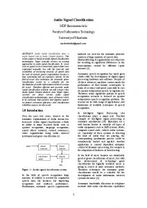
5.2. Performance versus WSR and SNR In order to observe WM decoding performance, performance at different WSRs has been examined for two-class classification. The SVM classifier is trained by an audio file of length about 139 sec. It is observed that the decoding performance does not depend on selection of the training data. Thus, test results reported in this section are obtained by the training data collected from a single audio clip. Distribution of TC versus WSR for un-compressed, MP3 compressed and AAC compressed files are compared and reported in Fig. 1 and Fig. 2. Note that, the FC ratios of Class 1(+1) and Class 2(-1) are obtained nearly the same, thus we reported the arithmetic mean of them. The SVM-based and correlation-based results are obtained by using a test set of length about 2.5 hours. As it is observed from Fig. 1 and Fig. 2, for un-compressed audio files, true classification performance of the correlation method and the SVM based method are similar and the decoding accuracy remains greater than 95% when WSR>-40 dB. However, the superiority of the proposed scheme can be seen in compressed domain. For the mp3 compressed audio, the proposed SVM–based decoding provides about 10% gain at WSR = -45 dB, while it is about 6% for the AAC compressed audio. In both compressed and un-compressed domain, TC ratio reaches to 100% for both decoding scheme when WSR ≥ -20 dB. In order to evaluate the WM decoding accuracy at noisy communication channels, the same test audio files are distorted by i.i.d. Gaussian noise. The reported performance is obtained on a test set of length about three hours. The SVM training is performed on a training set of length about 278 sec. As it is seen from Fig. 3, distribution of TC versus SNR is almost the same for correlation
based and SVM based decoding schemes. Decoding accuracy exceeds 90% at SNR = 15 dB, and reaches 99% at SNR = 20 dB. 6. CONCLUSION
This paper proposes a blind audio watermark decoding scheme based on supervised learning of the watermarked audio signals. Performance of the proposed decoder is superior to the classical correlation based method in both uncompressed and compressed domains. The developed watermark decoding method is also robust to channel noise.
REFERENCES [1] F. Hartung and M. Kutter, ”Multimedia Watermarking Techniques,” in Proc. of the IEEE, vol 87, no 7, pp. 10791107, 1999. [2] Y. Yaslan and B. Gunsel, “An Integrated Decoding Framework for Audio Watermark Extraction,” Proc. of the ICPR 2004, Cambridge, UK, 2004, pp. 879-882. [3] S. Sener and B. Gunsel, “Blind Audio Watermark Decoding Using Independent Component Analysis,” Proc. of the ICPR 2004, Cambridge, UK, 2004, pp. 875-878. [4] H. S. Malvar and D. F. Florencio, “Improved Spread Spectrum: A New Modulation Technique for Robust Watermarking,” IEEE Trans. On Signal Processing, vol. 51, no. 4, pp. 898-905, 2003. [5] Y. Fu, R. Shen and H. Lu, “Optimal Watermark Detection Based on Support Vector Machines,” Lecture Notes in Computer Science, vol. 3137, pp. 552-557, 2004. [6] S.Lyu and H. Fardi, “Detecting Hidden Messages Using Higher-Order Statistics and Support Vector Machines,” Lecture Notes in Computer Science, vol.2578, pp.340-354, 2002. [7] H. Ozer, I. Avcibas, B. Sankur, and N. Memon, “Steganalysis of audio based on audio quality metrics,” Proceedings of the IS&T/SPIE's 15th Annual Symposium on Electronic Imaging, vol. 5020, Santa Clara, CA, US, January 2003, pp.55-66. [8] V. N. Vapnik, Statistical Learning Theory: John Wiley, New York, 1998
Fig. 1. TC versus WSR for wav and mp3 files
Fig. 2. TC versus WSR for wav and AAC files.
Fig. 3. TC versus SNR.