automatic classification of audio data using nonlinear neural response ...

AUTOMATIC CLASSIFICATION OF AUDIO DATA USING NONLINEAR NEURAL RESPONSE MODELS J¨org-Hendrik Bach+ 

Arne-Freerk Meyer+

J¨orn Anem¨uller

Carl-von-Ossietzky University Oldenburg, Oldenburg, Germany † Colorado School of Mines, Golden, Colorado, USA

ABSTRACT Physiologically inspired feature extraction for audio classification often uses simplified parametric models of auditory processing. We employ linear and nonlinear neuron models directly derived from neural responses in zebra finches as feature extraction front-ends. The most important features were identified using automatic feature selection techniques. This allows both a quantitative evaluation of neural features for sound classification tasks in terms of classification accuracy and a qualitative analysis of the auditory features that are most relevant. It turned out that a relatively small subpopulation of neural responses is sufficient to achieve reasonable classification performance. For linear as well as for nonlinear neuron models, we found three different shapes of spectro-temporal features to be archetypical. The relation of these to analytic approaches (such as Gabor filters) is discussed. The overall classification rates in a 6-class task reached up to 94 % accuracy. Nonlinear models provided up to 15 % benefit over linear models, indicating the importance of nonlinearities in classification with physiologically motivated features. Index Terms— audio classification, biological systems, physiologically motivated feature extraction 1. INTRODUCTION Humans reliably identify many different classes of acoustic objects, despite considerable natural variability within each class and even in noisy and reverberant environments, factors that limit the performance of even the best classification algorithm. For this reason, science has been turning its attention towards biological systems, trying to mimic their processing in order to reach an equally high level of performance in identification of virtually any type of sensory stimulus. The most popular candidates of such physiologically motivated feature extractors in the auditory system are spectro-temporal filter approaches such as Gabor filters [1]. Simpler models only include temporal modulations (such as RASTA or Traps filters or amplitude modulation spectrograms [2, 3]) or only spectral modulations (such as mel-frequency cepstral coefficients). + These

Duncan McElfresh†

2. FEATURES We used predicted neural response rates as features for audio classification. The predictions are done by running the audio data through neuron models (Sec. 2.1), which have been trained using single-unit recordings from multiple auditory areas in male zebra finches for conspecific vocalizations1 as described in [7]. 2.1. Neural Model We employed the Linear-Nonlinear Poisson (LNP) cascade ([8], see Figure 1) as a model for neural reponses. It consists 1 freely

authors contributed equally to this work.

978-1-4673-0046-9/12/$26.00 ©2012 IEEE

These approaches have successfully been used in automatic speech recognition (ASR), non-speech audio classification and other fields. In this paper, we propose to use features directly derived from neural recordings from auditory areas. Neuron models based on the spectro-temporal receptive field (STRF) are used as feature extraction front-ends by implementing them as spectro-temporal filters. The parameters of the models are estimated using neural recordings from different auditory areas of zebra finches. Zebra finches are highly sensitive to natural sounds with spectro-temporal properties similar to human speech rendering them as suitable candidates to study auditory feature extraction [4]. We expect to obtain neural spectro-temporal representations that are comparable to those in humans. In addition to the linear estimate, we also implement more realistic nonlinear models in the form of a linear-nonlinear cascade. Approaches based on linear STRFs have previously been applied to ASR [5] and segmentation problems [6]. The features for object classification tasks are generated by predicting neural responses to acoustic stimuli using the obtained neural models. Feature selection is employed to identify the most salient STRFs for classification of a small set of everyday sounds. Modulation analysis and clustering in modulation space are used to identify clusters of STRFs that are similar in their shape and function.

357

available at http://crcns.org/

ICASSP 2012

2.3. Feature calculation




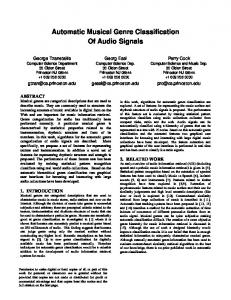
Fig. 1. The Linear-Nonlinear Poisson cascade model. (a) Linear features, (b) nonlinear features and (c) spikes created using a Poisson process implicitly assumed for STRF estimation. of a linear filter stage (STRF), followed by a static nonlinearity and a Poisson spike generation process. The STRF of a neuron acts as a matched filter and describes the acoustic pattern that elicits maximum response. The subsequent static memoryless function accounts for response nonlinearities and transforms the output of the linear stage into the instantaneous spike rate. For STRF estimation, a probabilistic model using an inhomogeneous Poisson process is assumed after the nonlinear stage. The Poisson assumption of independent spikes is a good approximation as long as the refractory period of the neuron is smaller than the temporal resolution of the neuron model (here: 2 ms). After training the LNP models with neural recordings, features can be extracted from audio data using the linear or nonlinear branch of the models (see Figure 1 (a) and (b)). 2.2. STRF estimation A well-known approach to estimate the STRF is reverse correlation between stimulus and response [8]. If the stimulus contains correlations across time or frequency the reverse correlation function Qsr can be decorrelated using the autocorrelation matrix Qss of the stimulus yielding [7] h = Q−1 ss Qsr .

(1)

Qsr and Qss are estimated as XXT and Xy, respectively, and h is the resulting estimate of the STRF of that specific neuron. X is the matrix that contains the stimulus vectors as columns and y is a vector containing the corresponding response values. Without loss of generality, X and y are assumed to have zero mean. To avoid overfitting along the undersampled stimulus dimensions a regularization scheme based on Principal Component Analysis (PCA) was used. As described in [8], the nonlinear function was estimated by dividing the output values of the model into N = 50 bins and mapping each bin to the mean value of the actual responses elicited by the corresponding stimulus examples. The nonlinearities were smoothed with a 5-point Gaussian window. Typical nonlinearities fitted this way often show tanh-like (compressive) or quadratic (expansive) shapes.

358

Of all available stimulus-response sets (199) we used those STRFs that produced a mean coherence between predicted and recorded spike rate greater than 0.25 resulting in 94 STRFs. The stimuli used in recording of the neural data contain most of their energy above 1 kHz. Consequently, the STRFs do not reflect any response patterns below 1 kHz. To cover low frequencies, too, we generated further STRFs by shifting the estimated STRFs by 5 channels (on a Bark scale) towards lower frequencies. The resulting 188 neuron models were used to compute auditory features as follows: the spectrogram of the audio input was correlated with each STRF to obtain the linear feature set. The nonlinear feature set was obtained by applying the corresponding static nonlinearity (cf. Figure 1 (b)) to the output of the linear stage. 3. FEATURE SELECTION To identify the most important STRFs, we used sequential forward search (SFS) with 5-fold cross-validation accuracy as cost function. SFS finds the single feature that provides best accuracy in the cross-validation task, keeps that one, and iteratively adds more features until the whole feature space is used up. For speed and simplicity, we used Naive Bayes classifiers in the process. The 188-dimensional feature space was processed in its entirety, resulting in a list of feature channels ordered by the importance of the corresponding neuron models. This is different to [5], where mutual information-based FS on linear STRF features was used to optimize phoneme recognition in ASR. 4. CLASSIFICATION Six classes of everyday sounds were used: speech (from the TIMIT database), telephone, coffee grinder, electrical toothbrush, water tap, and glass clinks (all from in-house recordings). Approximately 10 min of data per class was used for training, and 5 min for testing. Three different classifiers were used in this work: Naive Bayes (NB), Gaussian Mixture Models (GMM), and Support Vector Machines (SVM). NB classifiers assume a Gaussian distribution of the data and conditional independence of all feature dimensions (i.e., a diagonal covariance matrix). GMMs fit a set of Gaussian distributions to the data. In pilot experiments, we obtained the best results with diagonal covariance matrices and 10 components in each model. SVMs were trained using radial basis functions as kernels (“Gaussian” kernels). 5. RESULTS AND DISCUSSION Figure 2 shows the classification accuracy of all three classifiers over the number of features included. Using only one




    







 

 

 








   !


  



   

  
     





     

Fig. 2. Classification accuracy of all three classifiers over the number of features used. Dark lines show performance on linear features, light lines show performance on nonlinear features.







     





  









feature already results in 40–50 % accuracy (chance level for 6 classes is 1/6 ≈ 16.7 %). Performance increases with increasing number of features for all classifiers; however, NBs reach a peak with about 30 features at just below 70 % accuracy, GMMs saturate after 15–20 features at about 80 % accuracy. Only SVMs gain performance beyond 30 features. Experiments with linear-kernel SVMs showed rather poor performance (not shown). Feature selection was carried out using NB classifiers (and not individually for each classifier) due to computational cost. Since SVMs are discriminative classifiers, the features selected with NB classifiers are obviously better suited to NB and the similar GMM models than SVMs, which explains that SVMs start at a lower performance than GMMs. We expect that using SVM-based feature selection would shift the SVM curves towards earlier convergence at the same value (≈ 94 %). It turns out that a set of 15-20 neurons selected using FS is sufficient to attain good performance even with comparatively simple classifiers. This is significantly less than the 65 × 6 optimal STRFs found in ASR [5], which on the other hand contains more classes. NB and GMM seem to cope better with linear features than nonlinear ones, quite the opposite to SVMs. The nonlinear stage changes the distribution of the data to higher or lower kurtosis (corresponding to expansive and compressive nonlinearities, respectively), possibly violating the Gaussian assumption of the NB and, to a lesser extent, the GMM. Since the estimated nonlinearity maps the linear filter output onto a recorded spike rate which only assumes positive values, it has the additional effect of halfwave rectification. The resulting distribution of the features is highly asymmetric with a steep cut-off at zero, which is hard

     

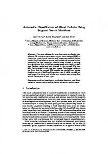
Fig. 3. Classification performance of the 6 best selected filters. Legend identical to Figure 2. Dark lines correspond to linear features, light grey lines to nonlinear features. The selected filters are plotted above (linear feature set) and below (nonlinear) the graph. Note that the pool of possible filters was identical for linear and nonlinear features, but different ones were chosen as salient in the feature selection process. to model with Gaussians. Correlation analysis of the STRFs revealed that the primarily selected filters are less correlated than those added later. Therefore the independence assumption of the NB is only met for the first few FS steps, which explains the low or even negative contribution of the later filters. Figure 3 is a zoom on Figure 2, showing the first 6 selected features and their actual filter shapes. It can be seen that both linear (top row) and nonlinear (bottom row) feature extraction cause similar types of filters to be selected: frequency-specific narrow-band filters, narrow- and broad-band onset detectors and temporal modulation filters, as well as sporadic more complex spectro-temporal patterns. Additionally, the downshifted STRFs are often selected, which is likely caused by the low-frequency content of some of the classes (the coffee grinder, for example). Figure 4 shows the space of temporal and frequency modulations covered by the STRFs. Each STRF is plotted as a dot at the position of its maximal modulation, i.e. the peak of the magnitude of the 2D Fourier transform of the timefrequency filter. Cluster analysis revealed the occurance of typical shapes: fitting a GMM to the distribution of the data in

359

in order to successfully learn from auditory processing, the apparent nonlinearities should not be neglected. 7. ACKNOWLEDGEMENTS The authors are indebted to Sarah Woolley and Thane Fremouw for providing the database of neural recordings. We also thank Angela Josupeit for conducting the first pilot experiments and Hendrik Kayser for fruitful discussion and for proofreading the manuscript. This work was supported by the DFG and the DAAD.



 

     !    " 



8. REFERENCES 

[1] S. Chu, S. Narayanan, and C.C.J. Kuo, “Environmental Sound Recognition With Time–Frequency Audio Features,” IEEE Tran. Aud. Sp. Lang., vol. 17, no. 6, pp. 1142–1158, 2009.

 








    

 





Fig. 4. Clustering of the STRF filters in modulation space. One blue dot for each STRF, orange dots refer to the first 20 STRFs as obtained in the linear feature selection task. Almost all of the 188 filters can be attributed to one of three major clusters whose centers are indicated by the green triangles. Exemplary STRFs located most closely to the center of these clusters are shown above the figure. They exhibit spectral (left), spectro-temporal (center) and temporal (right) modulations. modulation space results in three distinct clusters. Each Gaussian (green triangles labelled ‘center’) corresponds roughly to one of the three dominant shapes, a typical example of which is plotted above the cluster plot. We also experimented with higher numbers of clusters, which led to several of those to be lumped together to effectively form three clusters again. 6. CONCLUSION We demonstrated that spectro-temporal neural filters can be used to extract features from audio data with promising success in classification tasks. The employed nonlinearities in the neural models can improve performance significantly. Feature selection and clustering analysis showed that a small number of distinct typical shapes (purely temporal, purely spectral, diagonal, and more complex filters) are most relevant to distinguish everyday sounds. Some of these shapes are similar to parametric approaches such as Gabor filters, but others would not be captured by a comparatively simple filter bank. The nonlinearity of the model proved beneficial when classification rates reached competitive levels, indicating that

360

[2] A. Adami, L. Burget, S. Dupont, H. Garudadri, F. Grezl, H. Hermansky, P. Jain, S. Kajarekar, N. Morgan, and S. Sivadas, “Qualcomm-ICSI-OGI features for ASR,” in Proc. ICSLP, 2002, number 1, pp. 1–4. [3] J.-H. Bach, B. Kollmeier, and J. Anem¨uller, “Modulation-based detection of speech in real background noise: Generalization to novel background classes,” in Proc. ICASSP, 2010, pp. 41–44. [4] S.M.N. Woolley, T.E. Fremouw, A. Hsu, and F.E. Theunissen, “Tuning for spectro-temporal modulations as a mechanism for auditory discrimination of natural sounds.,” Nat. Neurosci., vol. 8, no. 10, pp. 1371–1379, 2005. [5] S. Thomas, K. Patil, S. Ganapathy, N. Mesgarani, and H. Hermansky, “A phoneme recognition framework based on auditory spectro-temporal receptive fields,” in Proc. Interspeech, 2010, pp. 2458–2461. [6] M. Coath and S.L. Denham, “Robust sound classification through the representation of similarity using response fields derived from stimuli during early experience,” Biol. Cybern., vol. 93, pp. 22–30, 2005. [7] P. Gill, J. Zhang, S.M.N. Woolley, T. Fremouw, and F.E. Theunissen, “Sound representation methods for spectrotemporal receptive field estimation.,” J. Comput. Neurosci., vol. 21, no. 1, pp. 5–20, 2006. [8] E. J. Chichilnisky, “A simple white noise analysis of neuronal light responses.,” Network, vol. 12, no. 2, pp. 199– 213, 2001.