the dynamics anonymity and joints stiffness/damping variations. ... a KUKA LWR moving in free space with its joints stiffness and damping vary with time in sine ...
Conference ISR ROBOTIK 2014
Robust Direct Adaptive Fuzzy Control of Flexible Joints Robots with Time-Varying Stiffness/Damping Parameters Ibrahim F. Jasim, Peter W. Plapper Faculty of Science, Technology, and Communication, University of Luxembourg, Luxembourg
Summary/Abstract In this article, we address the problem of controlling unknown flexible-joint robots with unknown time-varying stiffness and damping parameters. We propose a Robust Direct Adaptive Fuzzy Control (RDAFC) strategy that accommodates the dynamics anonymity and joints stiffness/damping variations. The RDAFC strategy relies on the synergy of the concepts of fuzzy logic approximation and the Sliding Mode Control (SMC). The fuzzy logic approximation relaxes the need for knowing the robot dynamics and the SMC accommodates the parameters variations. We also modify the RDAFC strategy to be suited to the KUKA Lightweight Robot (LWR) and propose a control strategy that can accommodates dynamics anonymity, uncertainty and joints elasticity variations. Experimental results are performed on a KUKA LWR moving in free space with its joints stiffness and damping vary with time in sine and cosine waveforms respectively. From the experiments, we can see that excellent tracking performance is obtained when using the RDAFC strategy despite the joints elasticity parameters time-variance and the robot dynamics unavailability.
1
Introduction
Flexible Joints Robots (FJR) are applied nowadays in many vital applications like industry, medicine, space, ...etc. Joints flexibility adds safer operation of robots for different applications. However, such joints flexility results in more complex control situations. Despite their complexity, the derivation of the control strategies for the FJR attracted interests of many researchers from all over the world. In the framework of singular perturbation, Spong et. al. proposed a control strategy that relies on the concept of integral manifold in realizing the strategy and promising results were obtained [1]. In the FJR, the number of variables is more than the control actions and this urged researchers of using model reduction along with the singular perturbation in enhancing the control performance of the FJR [2]. Simplified PD controller was efficiently used in controlling the FJR with compensating the joints friction torques [3]. In [4, 5, 6], adaptive control was employed in accommodating possible parameters uncertainty in the control problem of the FJR. H∞ control design was suggested for the FJR and the effect of the external disturbance was attenuated below a certain level [7]. In [8, 9, 10], universal approximators like fuzzy and neural systems were used in building control strategies for such robot systems and good performance was obtained despite the dynamics uncertainties. Online gravity compensation is proposed along with a PD controller and only the motor side position and velocity are needed [11]. Passivity-based control strategy is suggested that can guarantee stable performance for the FJR using the motor side position and stiffness torque feedback [12]. One of the most important aim of almost all researchers is to enable the robot mimicking the human in its behavior since such resemblance would enable the robot of doing
ISBN 978-3-8007-3601-0
more complex tasks. If we consider the assembly tasks as an application example, we can see that human operator can perform such tasks simply because of the human high capability of the environment recognition and excellent arm muscles control. If we focus on the arm muscles control, we can notice that a human operator changes his arm joints elasticity with time so that smoother and safer tasks are performed and possible environment elasticity are accommodated [13, 14]. Of course such a change in joints elasticity are done unintentionally and acquired with human experience. Furthermore, if the human performs a certain task and shifts to another one, then his arm joints elasticity may also be varied (unintentionally) to accommodate such a change (if required). Stemming from this motivation one may need the variation of the joints elasticity parameters in a robot according to the task requirements. A FJR is a nonlinear system and when we have the elasticity terms are time-varying, then we would have a time-varying nonlinear system. In this article we suggest a Robust Direct Adaptive Fuzzy Control (RDAFC) strategy for unknown FJR with timevarying stiffness/damping parameters. The fuzzy logic approximation and the Sliding Mode Control (SMC) are used in accommodating the dynamics anonymity and the time-variance of the joints elasticity. Then we modify the RDAFC strategy to be suited to the KUKA Lightweight Robot (LWR) with unknown time varying joints elasticity parameters. We will consider the current joint specific controller as a diffeomorphism that relates the the joints state variables (joints position and velocity) to the input added torques which results in an unknown mapping with time-varying parameters and the RDAFC strategy would be used in controlling such a robot system. The rest of the paper is organized as follows. In section 2, we describe the control problem in hand and section 3 will lodge preliminary concepts and definitions. In sec-
149
© VDE VERLAG GMBH · Berlin · Offenbach
Conference ISR ROBOTIK 2014
3
tion 4, the RDAFC strategy will be presented and section 5 will contain the RDAFC strategy for the KUKA LWR. Experimental validation will be shown in section 6 and section 7 will conclude the article with pinpointing the recommendations for future works.
2
Before exhibiting the main control strategy suggested in this paper, we will explain the concept of fuzzy logic approximators along with other preliminary concepts, properties and assumptions.
Problem Statement
3.1
A Flexible Joint Robot (FJR) can be described by the following dynamics [15]:
(2)
Where q ∈ Rn is the links position vector, M (q) ∈ Rn×n is the inertia matrix, C(q, q) ˙ q˙ ∈ Rn is the centripetal and Coriolis vector, G(q) ∈ Rn×n is the gravity vector, τm ∈ Rn is the torque vector produced by the actuator, K ∈ Rn×n is a diagonal matrix whose main diagonal elements ki are the joints stiffness, qm ∈ Rn is the actuator side position, D ∈ Rn×n is a diagonal matrix whose main diagonal elements di are the joints damping. ˙ One Suppose that x1 = q, x2 = q, ˙ x3 = θ, and x4 = θ. can describe (1) as: x˙ 1 x˙ 2 x˙ 3 x˙ 4
If u1 is Ai1 and u2 is Ai2 and... and u2n is Ai2n Then yf = yfi
yf = θT h(u)
(7)
with:
(3) where X ∈ R4×n : X = (x1 , x2 , x3 , x4 )T , f1 (X) = M −1 (x1 )(K(x3 − x1 ) + D(x4 − x2 ) − C(x1 , x2 )x2 − G(x1 )), f2 (X) = B −1 (K(x1 − x3 ) + D(x2 − x4 )), and g = B −1 . (3) can be written in the following compact form:
µi (u) =
2n Y
Aij (uj )
j=1
µ2 (u) µL (u) µ1 (u) , PL , ..., PL ) h(u) = ( PL i=1 µi (u) i=1 µi (u) i=1 µi (u)
X˙ = F (X) + G(τm + K(x1 − x3 ) + D(x2 − x4 )) (4)
µi (u) ≥ 0
with F (X) ∈ R4×n : F (X) = (x2 , f1 (X), x4 , f2 (X)) and G = (0, 0, 0, g)T . For time-varying damping/stiffness parameters, (4) would be:
L X
X˙ = F (X) + G(τm + K(t)(x1 − x3 ) + D(t)(x2 − x4 )) (5) For unknown robot dynamics, (5) results in unknown time-varying nonlinear system and the objective of this article is to propose a robust adaptive fuzzy controller for such kind of robot systems. We will consider the case of a KUKA Lightweight Robot (LWR) as a case study and modify the suggested strategy to be applicable to such a robot system with time-varying joints stiffness and damping parameters.
(6)
with i = 1, 2, ..., L; L is the total number of the If-Then rules; Aij (i = 1, 2, ..., L; j = 1, 2, ..., m) are the premise fuzzy sets; and yfi is crisp output of the k th rule. Through using a singleton fuzzifier along with the product inference, the overall output for the fuzzy system above can be computed as [16, 17]:
= x2 = f1 (X) = x4 = f2 (X) + gτm + K(x1 − x3 ) + D(x˙ 1 − x˙ 3 )
ISBN 978-3-8007-3601-0
Fuzzy Logic Approximators
One of the vital applications of the fuzzy set theory is the functions approximation. It gives a feasible way of approximating unknown smooth functions through the use of T-S fuzzy models. Suppose that we desire to approximate the control action of (5), and consider that (q1 , q˙1 , ..., qn , q˙n ) = (u1 , u2 , ...., u2n ). Let’s assume that the output of each mapping, that will be approximated, is yf . Such approximation would be feasible in the context of fuzzy If-Then rules as: Controller Rule i:
M (q)¨ q + C(q, q) ˙ q˙ + G(q) = K(qm − q) + D(q˙m − q) ˙ (1)
B q¨m + K(qm − q) + D(q˙m − q) ˙ = τm
Preliminaries
µi (u) > 0
i=1
and: θ = (yf1 , yf2 , ..., yfL ) Hence, the control action τm of (5) can be approximated through a fuzzy logic controller τf = (yf 1 , ..., yf n ) and this is called direct fuzzy control [17]. That is: τf (q, q|θ) ˙ = θT h(q, q) ˙
150
(8)
© VDE VERLAG GMBH · Berlin · Offenbach
Conference ISR ROBOTIK 2014
3.2
4
Properties and Assumptions
Below properties are common between robot manipulators [15]: P1. For all robot manipulators, M (q) is a positive definite and symmetric matrix. P2. For all robot manipulators, the matrix M˙ (q) − 2C(q, q) ˙ is a skew symmetric matrix, that is for all x ´ : x ´ ∈ Rn and x ´ 6= 0, we have x ´T (M˙ (q) − 2C(q, q))´ ˙ x = 0. Define the error vector to be: x ˜1,3 = x1,3 − xd1,d3
w = Fˆ (X|θ) − F (X)
(17)
The minimum approximation error w∗ is defined to be:
(10)
w∗ = Fˆ (X|θ∗ ) − F (X)
(11)
Where θ∗ is the optimal parameter vector of θ that is defined as:
with γ > 0. (10) can be rewritten as: s = x˙ 1,3 − x˙ r1,r3
Since the dynamics of the robot is assumed to be unknown then F (X), G, K(t), and D(t) would be unknown. We use the fuzzy logic in approximating F (X) and we will denote such an approximation as Fˆ (X|θ). Suppose that the approximation error is w, that is:
(9)
and consider the filtered error vector to be described as: s=x ˜˙ 1,3 + γ x ˜1,3
Robust Direct Adaptive Fuzzy Control (RDAFC) Design
where:
(18)
θ∗ = arg min|θ|∈Mθ [supX∈MX Fˆ (X|θ) − F (X)] (19) x˙ r1,r3 = x˙ d1,d3 − γ x ˜1,3
(12)
Note 1. It has been shown that the filtered error described by (10) has the following properties: (i) the equation s(t) = 0 defines the time-varying hyperplane in Rn , on which the tracking error vector x ˜1,3 decays exponentially to zero.(ii) if x ˜1,3 (0) = 0 and |s(t)| ≤ ε with constant ε, x ˜ (t) i−1 i−2 γ ε, i = 1, 2} for then x ˜1,3 (t) ∈ Ωε = { 1,3 x ˜1,3 ≤ 2 ∀t ≥ 0 and (iii) if x ˜1,3 (0) 6= 0 and |s(t)| ≤ ε then x ˜1,3 (t) (n−1) will converge to Ωε within a time constant of γ [18]. Taking the time derivative of (11), we obtain: s˙ = x ¨1,3 − x ¨r1,r3
(13)
Despite the robustness of the SMC, a possible chattering may deteriorate the control performance and may even drive the system to be unstable. Therefore, a modified filtered error [19] is introduced that can be expressed as: s sε = s − εtanh( ) ε
and Fˆ (X|θ) = θT h(q, q) ˙ Let’s introduce the following control action: ˆ −1 [−(w ¯ˆ 1 − x3 | + DG| ¯ˆ x˙ 1 τm = G ˆ + KG|x sε ˆ + X˙ d ] −x˙ 3 |)tanh( ) − Kd s − F (X|θ) ε
(22)
ˆ˙ = η2 sε τm G
(23)
(15) η3 |sε |
if(|w| ˆ < Mw ) or (|w| ˆ = Mw and w ˆ˙ = η3 |sε | ≤ 0) P (η |s |) if(| w| ˆ = Mw and 3 ε η3 |sε | > 0)
(16)
¯ and DG ¯ are the upper bounds of KG Suppose that KG and DG respectively. We will design the control strategy relying on the modified filtered error (14). However, before we proceed in explaining the suggested control strategy, below assumptions are needed to be satisfied: A1. The signals x1,3 , x˙ 1,3 , and x ¨1,3 are available for measurement. A2. The signals xd1,d3 , x˙ d1,d3 , and x ¨d1,d3 are bounded and piecewise continuous. A3. All joints stiffness and damping parameters are bounded.
ISBN 978-3-8007-3601-0
˙ θˆ = η1 sε h(q, q) ˙
(14)
and |di (t)| ≤ dui
(21)
with Kd = diag(kd1 , ..., kd2n ); kd1 , ..., kd2n are positive constants. The control action (21), with parameters update laws described by (22)-(26) below, can be shown to provide globally stable performance for the FJR described by (5). The parameters update laws are:
Let’s define k(t) = (k1 (t), ..., kn (t))T and d(t) = (d1 (t), ..., dn (t))T . All joints stiffness and damping are assumed to be bounded. That is: |ki (t)| ≤ kui
(20)
ˆ¯˙ = KG
151
η |s | 4 ε
(24)
ˆ¯ < M ) or if(|KG| KG ˆ¯ = M (|KG| KG and
η4 |sε | ≤ 0) ˆ¯ = M P (η |s |) if(| KG| 4 ε KG and η4 |sε | > 0)
(25)
© VDE VERLAG GMBH · Berlin · Offenbach
Conference ISR ROBOTIK 2014
and
ˆ¯˙ = DG
η5 |sε |
ˆ ¯ < MKG ) or if(|DG| ˆ ¯ = MDG and (|DG|
η5 |sε | ≤ 0) ˆ ¯ = MKG and P (η5 |sε |) if(|DG| η5 |sε | > 0)
τf (q, q|θ) ˙ = θT h(q, q) ˙ (26)
with Mw , MKG , and MDG are design parameters that ˆ ˆ ¯ and DG ¯ respectively. specify the bounds of w, ˆ KG, The stable performance of the strategy above can be shown through considering the Lyapunov candidate V = T 1 T ˜ ˜¯ ˜ 1 G ˜ T G+ ˜ 1 w ¯ KG+ ˜ T w+ ˜ 1 KG (sε sε + 1 θ˜T θ+ 2
2η1 T 1 ˜ ˜¯ ¯ 2η5 DG DG).
2η2
2η3
5
with Mq and Mq˙ are the allowable sets of q and q˙ respectively. Let’s introduce kˆu and dˆu to be parameter vectors compensating for ku and du respectively. We will assume that |w| ˆ ≤ Mw , |kˆu | ≤ Mk , and |dˆu | ≤ Md , i.e. the parameter vectors w, ˆ kˆu and dˆu are required to remain within prescribed sets. Let’s consider the control action to be composed of two terms; a fuzzy control action τf and a bounding term τb , that is:
2η4
Then it can be proved that the time derivative of this Lyapunov candidate is decreasing along the RDAFC control strategy above, i.e. V˙ ≤ −sTε Kd sε . Hence all closed loop signals are bounded with the modified filter to be zero within a small time constant as detailed in Note 1. Nextly, we will modify the RDAFC and make it suitable for one of the industrial robots which is the KUKA LWR.
RDAFC Strategy for The LWR
The dynamics of the KUKA LWR can be described by [21]: f (q, q, ˙ q¨) = τ + K(t)(qF RI − q) + D(t)(q˙F RI − q) ˙ (27) f (q, q, ˙ q¨) is the unknown dynamics function and qF RI is the desired position values. For the case of time-varying joints stiffness and damping, one can write (27) as: f (q, q, ˙ q¨) = τ + K(t)(qd − q) + D(t)(q˙d − q) ˙
∗
∗
w = τf (q, q|θ ˙ )−
∗ τm
Where θ∗ is the optimal parameter vector of θ that is defined as:
(34)
if(|dˆu | < Md ) or (|dˆu | = Md and ˙ˆ ˙ ε | ≤ 0) du = η2 |Zs ˆ ˙ P (η2 |Zsε |) if(du = Md and ˙ ε | > 0) η2 |Zs θ˙ = −η3 sTε h(q, q) ˙
w ˆ˙ =
(36)
(37)
η4 |sε |
if (|w| ˆ < Mw ) or (|w| ˆ = Mw and η4 |sε | ≤ 0) P (η4 |sε |) if (|w| ˆ = Mw and η3 |sε | > 0) (38)
where η1 , η2 , η3 , η4 > 0, Z ∈ Rn×n , Z = diag(qd1 − q1 , ..., qdn − qn ) and P (.) is the projection function, that is:
∗ θ∗ = arg min|θ|∈Mθ [supq∈Mq ,q∈M τ (q, q|θ ˙ ∗ ) − τm ] ˙ q˙ f (31)
ISBN 978-3-8007-3601-0
τb = −Kd s(t) − Γ(kˆu + dˆu + w) ˆ
˙ ε| η2 |Zs
(29)
(30)
(33)
Kd = diag(kd1 , kd2 , ..., kdn ) with kd1 , kd2 , ...,kdn are positive constants, and Γ = diag(tanh( εs11 ), tanh( εs22 ), ..., tanh( εsnn )). Therefore, the need for knowing the robot dynamics is relaxed through the use of the control action (33). In order to guarantee the stable performance for the suggested RDAFC strategy, the parameters vectors kˆu , dˆu , θ, and w ˆ are updated according to the following laws: η1 |Zsε | if(|kˆu | < Mk ) or (|kˆu | = Mk and ˙ ˆ (35) ku = η1 |Zsε | ≤ 0) ˆ P (η1 |Zsε |) if(|ku | = Mk and η1 |Zsε | > 0)
(28)
The minimum approximation error w∗ is defined to be:
τ = τf + τb Where:
In order to modify the RDAFC strategy to be applicable to the KUKA LWR, we introduce the error signal to be q˜ = q − qd and the filtered error to be s = q˜˙ + γ q˜. Likewise to the RDAFC strategy derived in section 4, we can say that s = q˙ − q˙r with q˙r = q˙d − γ q˜. Furthermore, we introduce the modified filtered error to be sε = s − εtanh( εs ). Now, let’s suppose that the control strategy that stabilizes (28) is described by τ ∗ . We propose a fuzzy controller τf that approximates such a stabilizing controller with w to be the error between τf and τ ∗ . That is: ∗ w = τf (q, q|θ) ˙ − τm
(32)
P (η1 |Zsε |) = η1 |Zsε | − η1 |Zsε |(
152
kˆuT kˆu ) |kˆu |2
© VDE VERLAG GMBH · Berlin · Offenbach
Conference ISR ROBOTIK 2014
Figure 1: (a) KUKA Lightweight Robot (LWR); (b)The waveforms of the KUKA LWR ith joint stiffness (blue) and damping (green).
˙ ε |) = η2 |Zs ˙ ε | − η2 |Zs ˙ ε |( P (η2 |Zs
P (η4 |sε |) = η4 |sε | − η4 |sε |(
dˆTu dˆu ) |dˆu |2
w ˆT w ˆ ) |w| ˆ2
The stability of the RDAFC strategy can be ascertained through considering the Lyapunov candidate V = 1 ˜T ˜ 1 T 1 ˜T ˜ 1 ˜T ˜ 1 ˜ T w, ˜ 2 sε M (q)sε + 2η1 ku ku + 2η2 du du + 2η3 θ θ+ 2η4 w with k˜u = kˆu − ku , d˜u = dˆu − du , θ˜ = θ − θ∗ and w ˜=w ˆ − w∗ and it can be shown that the time derivative of V is decreasing along the strategy above. Therefore, sε → 0 as t → ∞ and from (37) we can say that θ˙ → 0 as t → ∞. Hence, θ will be always bounded and there is no need to use the projection function used for the update laws of the other parameters. For (35), (36), and (38) the right hand side is greater than or equal to zero that may cause the proliferation of their parameters with time. Therefore, the use of the projection function was inevitable to force those parameters for remaining within a certain bound.
6
Experimental Results
In order to see the performance of the suggested RDAFC strategy, we used it in controlling a KUKA Lightweight Robot (LWR) with time-varying joints stiffness and damping parameters. The KUKA LWR is a 7-DOF industrial robot and the key features of the KUKA LWR is detailed in [22]. For research purposes, a Fast Research Interface (FRI) is available in the robot hardware that makes its joints control strategy customizable by the user through a C++ platform hence allowing researchers to apply their own control schemes in controlling the robot joints [20]. Through its platform, we programmed the joints stiffness and damping to vary in sine
ISBN 978-3-8007-3601-0
and cosine waveforms respectively, that is for the ith joint ki (t) = 20 + 10sin(t) and di (t) = 20 + 10cos(t). Figure 1.a shows the KUKA LWR that we used in our experiments and Figure 1.b shows the waveforms of the variations of the joints stiffness and damping parameters. Figure 2.a-f show the desired pose signals of the KUKA LWR end effector and the corresponding joint position signals are shown in Figure 3.a-g. The control actions when using the RDAFC strategy in commanding the joints of the given robot are shown in Figure 3.h-n. The RDAFC strategy was used with the following details: Kd = diag(15, 12, 12, 15, 10, 5, 4) εT = [0.005, 0.07, 0.06, 0.05, 0.04, 0.09, 0.04]T γ T = [80, 80, 80, 50, 12, 12, 5]T MkT = [2.3, 3.3, 2.0, 3.4, 2.4, 2.2, 2.2]T MdT = [2.1, 3.0, 3.0, 2.0, 2.0, 2.0, 1.7]T MwT = [0.002, 0.017, 0.007, 0.0005, 0.0007, 0.00012 , 0.0007]T η1 = 0.001, η2 = 0.01, η3 = 0.0001, and η4 = 0.0001. Gauss membership functions of the form: Aij (uj ) = exp(−
(uj − c)2 ) 2σ 2
(39)
are used in the premise of the ith If-Then rule of the RDAFC. c and σ are the center and width of the gauss membership function. The joints position and velocity, say q and q˙ respectively, are considered the input variables for the fuzzy logic controller, and each one of those state variables is assigned with two membership functions for the premise part of the if-then rules. For simplicity, we will describe each Gauss membership function described by (39), with an ordered pair (c, σ). Below are the parameters of the fuzzy sets of the variables considered in the RDAFC, say q and q: ˙ q1 : (−0.7, 0.0849) and (−0.9, 0.0849) q2 : (−0.4, 0.0849) and (−1, 0.0849) q3 : (0.3, 0.0849) and (0.2, 0.0849) q4 : (1.6, 0.0849) and (1.2, 0.0849)
153
© VDE VERLAG GMBH · Berlin · Offenbach
Conference ISR ROBOTIK 2014
Figure 2: The manipulated object signals: (a) x (in mm); (b) y (in mm); (c) z (in mm); (d) Θ (in degree); (e) Ψ (in degree); (f) Φ (in degree); (g) ex (in mm); (h) ey (in mm); (i) ez (in mm); (j) eΘ (in degree); (k) eΨ (in degree); (l) eΦ (in degree).
Figure 3: Joints position and velocity signals: (a) qd1 (in mrad); (b) qd2 (in mrad);(c) qd3 (in mrad); (d) qd4 (in mrad); (e) qd5 (in mrad); (f) qd6 (in mrad); (g) qd7 (in mrad); (h) τ1 (in N.m); (i) τ2 (in N.m); (j) τ3 (in N.m); (k) τ4 (in N.m); (l) τ5 (in N.m); (m) τ6 (in N.m); (n) τ7 (in N.m); (o) q˜˙ 1 (in mrad); (p) q˜˙ 2 (in mrad); (q) q˜˙ 3 (in mrad); (r) q˜˙ 4 (in mrad); (s) q˜˙ 5 (in mrad); (t) q˜˙ 6 (in mrad); (u) q˜˙ 7 (in mrad). q5 : (−0.1, 0.0849) and (−0.4, 0.0849) q6 : (−0.7, 0.0849) and (−1.1, 0.08494) q7 : (−2, 0.0849) and (−2.3, 0.0849) q˙1 : (0.14, 0.0849) and (−0.1, 0.0849) q˙2 : (0.6, 0.0849) and (−0.5, 0.0849) q˙3 : (0.05, 0.0849) and (−0.06, 0.0849) q˙4 : (0.3, 0.0849) and (−0.3, 0.0849) q˙5 : (0.3, 0.0849) and (−0.6, 0.0849) q˙6 : (0.4, 0.0849) and (−0.6, 0.0849) q˙7 : (0.6, 0.0849) and (−0.2, 0.0849) As per using the suggested RDAFC control strategy in section 5, the joints control actions were graphed in Fig-
ISBN 978-3-8007-3601-0
ure 3.h-n that resulted in the joints position error signals shown in Figure 3.o-u. We can see that the RDAFC strategy is of excellent joint space performance. Figure 2.g-l show the pose error signals and we can notice that the excellent joint space tracking performance had a direct reflection on that of the task space. Furthermore, we graphed the filtered error and the modified filtered error and as shown in Figure 4. Figure 5 shows the estimate of the ith joint approximation error w ˆi , stiffness bound kui , and damping bound dui . We can see that all signals involved in the design are bounded and excellent tracking performance is achieved despite the time variance of the
154
© VDE VERLAG GMBH · Berlin · Offenbach
Conference ISR ROBOTIK 2014
Figure 4: Joints filtered error and modified filtered error: (a)s1 ; (b) s2 ; (c) s3 ; (d) s4 ; (e) s5 ; (f) s6 ; (g) s7 ; (h) sε1 ; (i) sε2 ; (j) sε3 ; (k) sε4 ; (l) sε5 ; (m) sε6 ; (n) sε7 ;
Figure 5: (a)w ˆ1 ; (b) w ˆ2 ; (c) w ˆ3 ; (d) w ˆ4 (e) w ˆ5 ; (f) w ˆ6 ; (g) w ˆ7 ; (h) kˆu1 ; (i) kˆu2 ; (j) kˆu3 ; (k) kˆu4 ; (l) kˆu5 ; (m) kˆu6 ; (n) ˆ ˆ ˆ ˆ ˆ ˆ ˆ ˆ ku7 ; (o) du1 ; (p) du2 ; (q) du3 ; (r) du4 ; (s) du5 ; (t) du6 ; (u) du7 . joints stiffness and damping parameters.
7
Conclusion
The control problem of the Flexible Joint Robots (FJR), with unknown dynamics and unknown time-varying joints stiffness and damping, was addressed and a Robust Direct Adaptive Fuzzy Control (RDAFC) strategy is proposed for such robot systems. RDAFC strategy is a synergy of the concepts of fuzzy logic approximation and the Sliding Mode Control (SMC). The fuzzy approximator relaxes the need for knowing the robot dynamics and the SMC accommodates the variations of the joints
ISBN 978-3-8007-3601-0
elasticity parameters. Then we modify the RDAFC strategy to be suited for the KUKA Lightweight Robot (LWR) with the joints stiffness and damping parameters to be time-variant. The stable performance of the suggested RDAFC strategy is shown and experiment is performed on the KUKA LWR with varying the joints stiffness and damping in sine and cosine waveforms and the efficiency of the suggested approach is shown.
8
Acknowledgement
This work is supported by the Fonds Nationale de Recherche (FNR) in Luxembourg under grant no. AFR
155
© VDE VERLAG GMBH · Berlin · Offenbach
Conference ISR ROBOTIK 2014
2955286.
References
[11] De Luca, A.; Siciliano, B.; Zollo, L.: PD control with on-line gravity compensation for robots with elastic joints: theory and experiments, Automatica, Vol. 41, pp.1809-1819, 2005.
[1] Spong, M.W.; Khorasani, K.; Kokotovic, P.V.: An integral manifold approach to the feedback control of flexible joint robots, IEEE Journal of Robotics and Automation, Vol. RA-3, No. 4, pp.291-300, 1987.
[12] Albu-Schäffer, A.; Ott, C.; Hirzinger, G.: A unified passivity-based control framework for position, torque and impedance control of flexible joint robots, International Journal of Robotics Research, Vol. 26, No. 1, pp.23-39, 2007.
[2] Siciliano, B.; Book, W.J.: A singular perturbation approach to control of lightweight flexible manipulators, International Journal of Robotics Research, Vol. 7, No. 4, pp.79-90, 1988.
[13] Perreault, E.J; Kirsch, R.F.; Crago, P.E.: Multijoints dynamics and postural stability of the human arm, Experimental Brain Research, Vol. 157, pp.507-517, 2004.
[3] Lozano, R.; Valera, A.; Albertos, P.; Arimoto, S.; Nakayama, T.: PD control of robot manipulators with joint flexibility, actuators dynamics and friction, Automatica, Vol. 35, pp.1697-1700, 1999.
[14] Sakaguchi, S.; Venture, G.; Azevedo, C.; Hayashibe, M.: Active joint visco-elasticity estimation of the human knee using FES, Proceedings of the 2012 IEEE/EMBS International Conference on Biomedical Robotics and Biomechatronics, 2427 June, pp.1644-1649, 2012.
[4] Khorasani, K.: Adaptive control of flexible-joint robots, IEEE Transactions on Robotics and Automation, Vol. 8, No. 2, pp.250-267, 1992. [5] Nicosia, S.; Tomei, P.: Output feedback control of flexible joint robots, Proccedings of the 1993 IEEE International Conference on Systems, Man, and Cybernetics, Le Touquet-France, 17-20 October, pp.700-704, 1993. [6] Lin, T.; Goldenberg, A.: Robust adaptive control of flexible joint robots with joint torque feedback, Proccedings of the 1995 IEEE International Conference on Robotics and Automation, Nagoya-Japan, 21-27 May, pp.1229-1234, 1995. [7] Moghaddam, M.: On robust H∞ -based control design for flexible joint robots, Proccedings of the 1996 IEEE International Conference on Control Applications, Dearborn-MI, 15-18 September, pp.522-527, 1996. [8] Malki, H.A.; Misir, D.; Feigenspan, D.; Chen, G.: Fuzzy PID control of a flexible-joint robot arm with uncertainties from time-varying loads, IEEE Transactions on Control Systems Technology, Vol. 5, No. 3, pp.371-378, 1997. [9] Tang, W.; Chen, G.; Lu, R.: A modified fuzzy PI controller for a flexible-joint robot arm with uncertainties, Fuzzy Sets and Systems, Vol. 118, pp.109119, 2001. [10] Chatalanagulchi, W.; Meckl, P.H.: Intelligent control of a two-link flexible-joint robot, using backstepping, neural networks, and direct method, Proceedings of the 2005 IEEE/RSJ International Conference on Intelligent Robots and Systems, AlbertaCanada, 2-6 August, pp.1594-1599, 2005.
ISBN 978-3-8007-3601-0
[15] Spong, M; Hutchinson, S.; Vidyasagar, M.: Robot Modeling and Control, John Wiley and Sons,Inc.,2006. [16] Wang, L.X.: Adaptive Fuzzy Systems and Control: Design and Stability Analysis, Prentice-Hall, Englewood Clifs, NJ, 1994. [17] Spooner, J.; Maggiore, M.; Ordonez, R.; Passino, K.: Stable Adaptive Control and Estimation for Nonlinear Systems: Neural and Fuzzy Approximator Techniques, John Wiley Sons, 2002. [18] Slotine, J.-J.: Sliding controller design for nonlinear systems, International Journal of Control, Vol. 40, pp.435-448, 1984. [19] Jasim, I.F.: Improved observer-based robust adaptive control for a class of nonlinear systems with unknown deadzone, Proceedings of the IMechE Part I: Journal of Systems and Control Engineering, Vol. 227, No. 2, pp.184-197, 2013. [20] Bischoff, R.; Kurth, J.; Schreiber, G.; Koeppe, R.; Albu-Schäffer, A.; Beyer, A.;Eiberger, O.; Haddadin, A.; Stemmer, A.; Grunwald, G.; Hirzinger, G.: he KUKA-DLR Lightweight Robot arm-a new reference platform for robotics research and manufacturing, Proceedings of the 41st ISR/Robotik 2010, Munich-Germany, 7-9 June, pp.1-8, 2010. [21]
KUKA Fast Research Interface 1.0, Version: KUKA.FRI 1.0 V2 en, KUKA Roboter GmbH, 16 September, 2011.
[22] Lightweight Robot 4+ Specification, Version: Spez LBR 4+ V5 en, KUKA Roboter GmbH, 22 December, 2011.
156
© VDE VERLAG GMBH · Berlin · Offenbach