Hybrid Fuzzy Adaptive Control of LEGO Robots Ján Vaščák Department of Cybernetics and Artificial Intelligence, Technical University in Košice, Letná 9, 042 00 Košice, Slovakia, E-mail:
[email protected]
Abstract: The main drawback of "classical" fuzzy systems is the inability to design and maintain their database. To overcome this disadvantage many types of extensions adding the adaptivity property to those systems were designed. This paper deals with one of them a new hybrid adaptation structure, called gradient-incremental adaptive fuzzy controller connecting gradient-descent methods with the so-called self-organizing fuzzy logic controller designed by Procyk and Mamdani. The aim is to incorporate the advantages of both principles. This controller was implemented and tested on the system of LEGO robots. The results and comparison to a 'classical' (non-adaptive) fuzzy controller designed by a human operator are also shown here. Keywords: Fuzzy adaptive controller, Gradient-descent methods, Jacobian, Gradientincremental adaptation.
1. Introduction Fuzzy logic has found many successful applications, especially in the area of control, but there are some limits of its use that are connected with the inability of the knowledge acquisition and adaptation to changed external conditions or parameters of the controlled system. To overcome this problem there were published lots of papers, e.g. [4, 9, 10], which deal with structures of Adaptive Fuzzy Controllers (AFC) using mostly approaches based on many variations of gradient-descent methods, the least square method [8], linear and non-linear regression or the linguistically based rule extraction. Of course, this list would be incomplete without mentioning neural networks and evolutionary algorithms [13]. Further, we will focus our attention only on 'pure' AFC. The main reason why to deal with this type of AFC is that they are with their nature and calculus the most similar systems to the non-adaptive (classical) FC. The properties of FC are well known, more than in the case of neural networks or genetic algorithms, in general. Fuzzy logic is able to simulate the human vague thinking very efficiently and therefore it seems to be very advantageous only to add the ability of the
knowledge acquisition to 'classical' fuzzy systems and nearby to preserve their properties. In this paper we will show the design of a hybrid control structure compound from two essential adaptation ways the well known Gradient-Descent Adaptation (GDA) and the so-called Self-Organizing Fuzzy Logic Controller (SOFLC) proposed by Procyk and Mamdani [11] with the aim to connect their advantages. In the section 6 we will show the implementation of this controller into the LEGO robots as well as some experiments with the evaluation of its efficiency.
2. Adaptation principles of fuzzy controllers The adaptation task of FC consists in the adjusting parameters of its knowledge base to fulfill the general goal of control, i.e. to eliminate the difference between the desired w(k) and real output y(k) of the system to be controlled. In other words to eliminate the control error e(k)=w(k)-y(k) (k as sampling step related to the time t, t=T.k where T is the sampling period). Other criteria concerning, e.g. transition time, energy consumption, overshoots, etc. can be taken into consideration, too. In principle, the values of knowledge base parameters can be obtained in two ways: either by identifying the parameters of the controlled system or by measuring the control quality. The first way defines the so-called parameter-adaptive systems and the second one performance-adaptive systems. In the first case, the information about the controlled system obtained in such a way is then to be transformed into the form of fuzzy rules of the controller. Therefore the methods of this kind are known as indirect methods, too (see [1, 6]). The performance adaptive systems transform the measured control quality directly to the controller parameters excluding the need of the system identification. They enable also to include another criteria where the minimal control error (control task) seems to be only a special criterion. The methods mentioned in the above are able to adjust either the parameters of membership functions (MF) or structure of rules or both. Mostly, they differ from the calculus used or other restriction conditions (type of MF, rule structure, etc.). However, most of them are based on minimizing the control error. As a gradient determines the shortest "descent" of this error in accordance on the knowledge base parameters it seems to be the most powerful adaptation method if there are no such application-dependent circumstances avoiding its use. SOFLC is also a special form embedding this calculus since it utilizes Jacobian what can be seen very clearly in (4). In the following we will describe both GDA and SOFLC used in our hybrid structure that can be included to direct methods.
3. Gradient-descent based adaptation of the knowledge base Each GDA is based on searching for a minimum (in the best case for the global one) of the error function E(k). We will define it as E(k)=e(k)2/2 and for the sake of simplicity we will omit the sampling step k in several formulae. Individual methods differ from one another by searching the minimum, defining the learning factor or other restriction conditions concerning, e.g. the shape of MF, etc. We will describe two ways of GDA here. Let us consider a TSK controller (Takagi-Sugeno-Kang) with n inputs xi and one output u of the j-th constant value bj (u=bj) with the product operator as the aggregation operator as well as MF in the symmetrical triangular form characterized by its center ai,j and support si,j (limit points of the support are ai,jsi,j/2 and ai,j+si,j/2) where i and j denote the i-th input and the j-th linguistic value for this input, respectively [2]. If there each input variable xi has li linguistic values and the output variable m values then we will get in total m + 2.TN parameters where TN = ll + … + ln is the total number of input MF. It can be proved their partial derivatives are in the form of (1) [5] where p = 1, ..., Nbj refer to all rules with the consequent bj and p = 1, …, NAij to all rules with MF Ai,j in their premises. Nr is the total number of rules and αp is the strength of the p-th rule.
Δa i , j
N Ai , j ⎛ N Ai , j ⎞ ⎜ ∑α p ⋅ bp − y ⋅ ∑α p ⎟ ⎜ p =1 ⎟ p =1 ⎠ = 2 ⋅ ( w − y ) ⋅ sgn( x i − a i , j ) ⋅ ⎝ N r ∑ α p ⋅ si , j ⋅ μ Ai , j ( xi ) p =1
Δs i , j
N Ai , j ⎛ N Ai , j ⎞ ⎜ ∑α p ⋅ bp − y ⋅ ∑α p ⎟ ⎜ p =1 ⎟ p =1 ⎠ = ( w − y ) ⋅ (1 − μ Ai , p ( xi )) ⋅ ⎝ N r ∑ α p ⋅ si , j ⋅ μ Ai , j ( xi ) p =1
Nb j
Δb j
=
∑α p =1
p
⋅ (w − y)
Nr
∑α p =1
p
(1)
It is evident the knowledge base parameters to be adjusted are ai,j, si,j and bj. If we compute partial derivatives of E(k) by these parameters in each sampling step k then considering the well known properties of the gradient we will get for next step k+1 the following values of ai,j, si,j and bj as shown in (2).
a i , j (k + 1) = a i , j ( k ) + K a ⋅ Δa i , j (k ) s i , j ( k + 1) = s i , j (k ) + K s ⋅ Δs i , j (k ), bi , j (k + 1)
=
(2)
bi , j (k ) + K b ⋅ Δbi , j (k )
where Ka, Ks and Kb are the learning factors. If we introduce an additional condition of maintaining fuzzy partitions and ai,j < ai,2 < … < ai,li [3] then the support si,j will be given by ai,j+1 – ai,j-1 and the system of equations (1) will be modified as described in (3) where r = 1, …, Nr.
⎧ y−w ⎡ μ A ( xi ) ⎪ ⋅ ⎢ i, j ⋅ ⎪ ai , j − ai , j −1 ⎢⎣ μ Ai , j −1 ( xi ) ⎪ N Ai , j −1 N Ai , j ⎤ ⎪⋅ ⋅ − − ⋅ − α ( b y ) α ( b y ) ⎥ ∑ ∑ p p p p ⎪ p =1 p =1 ⎥⎦ ⎪ ⎪if ai , j −1 < xi < ai , j ; ⎪ Δα i , j = ⎨ y − w ⎡ μ Ai , j ( xi ) ⋅ ⋅ ⎢ ⎪ ⎪ ai , j − ai , j +1 ⎢⎣ μ Ai , j +1 ( xi ) N Ai , j ⎪ N Ai , j +1 ⎤ ⎪⋅ α ⋅ ( b − y ) − α ⋅ ( b − y ) ⎥ ∑ p p p p ⎪ ∑ p =1 p =1 ⎥⎦ ⎪ ⎪if ai , j < xi < ai , j +1 ; ⎪⎩0 otherwise . Δbr = α r ⋅ ( y − w)
(3)
This method in contrast to (1) avoids generating uncovered parts of the universe of discourse by MF and shows mostly a better convergence. Further, the total number of parameters is Nr + TN and in most cases less than in (1) (if m + TN > Nr).
4. Structure of SOFLC The control circuit with a performance-adaptive AFC known as SOFLC is shown in fig. 1. As already mentioned this structure enables incorporating also another criteria than only the minimal control error. Control criteria are contented in the block of performance measure where the quality is evaluated by the performance index p(k) which expresses the magnitude and direction of changes to be performed in the knowledge base of the controller. The basic design problem of AFC consists in the design of M, where for each time sample t=K.T (K=0,1, …) a simplified incremental model of the controlled system M=J.T (J - Jacobian) is computed. It represents a supplement to the original model to reach a zero control error and is analogous to the linear approximation of the first order differential equation or in other words to gradients, too. As Jacobian (4) is a determinant of all first derivatives of the system with n equations f1, …, fn of n input variables x1, …, xn it means J is equal to the determinant of the dynamics matrix, i.e. it is a numerical value describing all n gradients in the sense of a characteristic value.
Figure 1: Self-organizing fuzzy logic controller. Now we need to transform this incremental description of a controlled system to the description of a controlling system, i.e. a controller. Considering the properties of the feed back connection we can see that y(k) ≈ e(k) (w(k) is known). As inputs and outputs of a controlled system change to outputs and inputs of a controller, respectively we can get the controller description like the inverse function of y(k) = fM(u(k)), i.e. the model of the controller is u(k) = f-1M(y(k)). Because J is a number, then M-1 is the reverse value of J.T. The reinforcement value r(k) is computed as r(k) = M-1.p(k).
J
=
∂f1 ∂x1 ∂f n ∂x1
∂f1 ∂x2 ∂f n ∂x2
L M L
∂f1 ∂xn ∂f n ∂xn
grad f1 =
L
(4)
grad f n
The knowledge base adaptation can be either relation-based or rule-based. For our purposes we will use the second way of adaptation. In general (for both methods), it is based on removing such rules Rnew(k) that caused a 'bad' control in the previous time step Rbad(k) and including new 'reinforced' rules, i.e. for next time step k+1 we will get:
R(k + 1) = ( R(k ) I Rbad (k )) U Rnew (k )
(5)
Each fuzzy rule rp (p = 1, …,Nr) of n inputs and one output represents their Cartesian product and is also a fuzzy relation Rp = A1,p x … x An,p x Bp. The knowledge base R is then a union of such rules (fuzzy relations) and after substituting into (5) it will be changed to (6). Rbad(k) can be a union of all previously fired rules, too. However, for the sake of simplicity we will consider only one rule with the greatest strength α and therefore Abad1 x … x Abadn is its premise. Reinforcement value r(k) corrects only the consequent of such a rule and Bnew is the fuzzified result of y(k)+r(k), i.e. fuzz(y(k)+r(k)). The simplest fuzzification is in the form of singletons but in general, other forms are possible, too. B
⎡ Nr ⎤ bad ⎢U ( A1, p ∩ A1 ) x K x An , p x B p ⎥ U ⎣ p =1 ⎦ Nr ⎡ ⎤ K U ⎢U A1, p x K x ( An , p ∩ Anbad ) x B p ⎥ U ⎣ p =1 ⎦ R ( k + 1) = ⎡ Nr ⎤ U ⎢U A1, p x K x An , p x ( B p ∩ B bad ) ⎥ U ⎣ p =1 ⎦ bad bad new U ( A1 x K x An x B ) 1444424444 3 Rnew
(6)
5. Hybrid gradient-incremental adaptive fuzzy controller In the above-described methods have their advantages and also drawbacks. GDA should be the fastest adaptation and it should converge after the minimal number of steps. However, there are two basic problems. First, an error function E(k) may be of a complex shape and hereby characterized by a number of local minima. It is very difficult in advance to estimate their number and possible place of the global minimum, i.e. optimal solution. Further, the absence of such estimation disables the determination of the learning factor value, too. If it is too small the convergence will be too slow and if it is too big there will be a risk the global minimum will be 'jumped over'. Secondly, there is possibility to minimize only one criterion – error function but in the practice there are also other control criteria. SOFLC is more practice-oriented but it is sensitive to external signals such as disturbances, noises and set-point changes because of their inability to distinguish whether the parameters of the controlled system are changed or an external signal entered the system. A negative effect can occur if the adaptation proceeds although it is not more necessary. So some wrong changes in the knowledge base may be performed. This state is caused by the wrong understanding if e.g. an external error occurs and AFC will evaluate it as a parameter change. Therefore, we tried to connect these two methods to one hybrid MISO structure to avoid their drawbacks as seen in the fig. 2 and named it as Gradient-Incremental adaptive Fuzzy Controller (GIFC).
Figure 2: Structure of a gradient-incremental adaptive fuzzy controller. The adaptation process can be described in following steps: 1. Definition of input and output variables 2. Defining of term sets for variables in the step 1
3. Design of initial membership functions (not necessary) 4. Processing GDA by (3) until the threshold of e(k) is reached 5. Processing SOFLC until the control error is greater than the threshold of e(k) 6. Processing GDA by (1) until the threshold is reached and repeated switching to the step 5 The main idea is that GDA is the fastest method if the threshold of the control error as the most important criterion is not too strict. In such a case we can choose a greater learning factor and speed up the adaptation. After this 'rough' adaptation we can switch the control to SOFLC to minimize the control error to be as small as possible and at this same time to include other criteria, too. GDA by (3) maintains fuzzy partitions. This condition owns several suitable properties but on the other hand side it is certain restriction in the adaptation process. Therefore, SOFLC does not hold this condition. However, if the control error increases again it will not more possible to switch adaptation to GDA by (3). From this reason it will be switched to GDA by (1). From (6) it is evident the so-called problem of rule expansion can occur as each 'bad' rule can be replaced by up to n+1 new rules, i.e. if in each step just one rule is replaced the knowledge base will be expanded by n further rules. To prevent this effect a garbage collection mechanism was designed. Its task is to remove replaced and identical rules. If there are rules with identical premises but different consequents occur the older rule will be removed.
6. Experiments The proposed hybrid control algorithm GIFC was implemented and tested on LEGO robots. Its results were compared also with a non-adaptive FC designed by a human operator. The control task was the so-called parking problem, i.e. to park a mobile robot at a given place and direction. This task was solved with and without obstacles. The process monitor (see fig. 2) evaluates the parking process by two criteria: parking error EP - more important corresponding with the control error and trajectory error ET- considered only in SOFLC which is computed as division of the real trajectory length and optimal trajectory length. The optimal trajectory is the shortest distance between the robot and the goal. The first criterion is in the form:
E P = (φ f − φ ) 2 + ( x f − x ) 2 + ( y f − y ) 2
(7)
where (x,y) are coordinates of the robot φ is the turning angle of wheels and (xf, yf, φf) are position and direction of the goal (parking place). Similar description is used for starting (initial) points, too.
In the case of obstacles the strategy of their avoiding depends on two light sensors. The existence of an obstacle is determined (supposed) if the light intensity of at least one sensor decreases under given threshold. There are two possibilities either the left or right direction and such a direction is chosen where the light intensity is higher. It supposes this way is shorter than another one to go round the obstacle. If the light intensity of both sensors is equal then the direction may be chosen randomly. In this case it is possible to define still one criterion - number of impacts on the obstacle. In figures 3, 4 and 5 results of several experiments for different starting points are depicted.
Figure 3: Comparison of trajectories for a non-adaptive FC (20, 80, 260) (a) and GIFC (20, 80, 260) (b).
Figure 4: Comparison of trajectories with an obstacle for a non-adaptive FC (60, 70, 150) (a) and GIFC (80, 80, 260) (b). In the table 1 we can see that first two criteria EP and ET are better fulfilled at a non-adaptive FC. There are two reasons. First, EP and ET are not totally independent. Both are quantitative and EP influences ET directly proportionally. If EP increases then also the trajectory will be more different from the optimal length but the shape may be in spite of that of 'better' what is also this case. It can be seen especially at the obstacle avoidance fig. 4 and 5. This assertion is supported by a smaller number of impacts at GIFC than at non-adaptive FC. Secondly, reinforced
rules are fired till in next steps after the error already occurred and in such a way delay influences the efficiency of GIFC negatively. Shortening the sampling period T can eliminate this problem. There are only hardware limitations.
Figure 5: Comparison of trajectories with an obstacle for a non-adaptive FC (80, 80, 260) (a) and GIFC (40, 80, 110) (b). Type NAFC GIFC NAFC GIFC
EP 0.407 6.545 0.568 4.706
ET 1.131 1.162 1.450 1.521
Number of impacts 3.15 1.33
Table 1: Comparison of the control quality for non-adaptive FC (NAFC) and GIFC. Conclusions The principal advantage of this approach is the substitution of a human expert in the design of a fuzzy controller, which is the most serious disadvantage of standard fuzzy systems. The design presented enables fuzzy systems to move in an unknown outer area that can be changed, e.g. autonomous vehicles among obstacles. Experiments showed that the most important criterion of number of impacts is better than at non-adaptive FC designed by a human operator. The quality of other two criteria may be improved by reinforcing the garbage collection mechanism. Many rules are not yet removed from the knowledge base and they are more information noise than contribution. It is possible to improve it by removing rules with MF their average grade of membership is small further by merging rules with similar premises or by considering partial contradiction of rules with identical premises. This experiment only demonstrated potential of such a method. It seems there may be many application cases of its use, for instance in aviation like discussed in [7] or in situational control [9].
References [1]
W. L. Baker, J. A. Farrell, “An introduction to connectionist learning control system,” IN: D. A. White, D. A. Sofge (Eds.), Handbook of Intelligent Control-Neural, Fuzzy and Adaptive Approaches, van Nostrand Reinhold Inc., New York, 1992.
[2]
H. Bersini, J.P. Nordvik, A. Bonarini, “A simple direct adaptive fuzzy controller derived from its neural equivalent,” see IEEE, 1993, pp. 345-350.
[3]
F. Guély, P. Siarry, “Gradient descent method for optimizing various fuzzy rule bases,” see IEEE, 1993, pp. 1241-1246.
[4]
C. J. Harris, C. G. Moore, “Intelligent identification and control for autonomous guided vehicles using adaptive fuzzy-based algorithms,” Engineering Applications of Artificial Intelligence 2, 1989, pp. 267-285.
[5]
R. Jager, Fuzzy Logic In Control (PhD. thesis), Technical University of DELFT, Holland, 1995.
[6]
Y. T. Kim, Z. Bien, “Robust self-learning fuzzy controller design for a class of nonlinear MIMO systems,” Int. Journal Fuzzy Sets and Systems, Elsevier Publisher, Holland, N. 2, Vol. 111, 2000, pp. 17-135.
[7]
P. Kováčik, H. Tóth: Artificial Neural Nets and Parametric Aeroplane Control, In: 2nd Slovak Conference on artificial neural networks, 1012.11.1998, Smolenice, s.83-88.
[8]
M. Ma, Y. Zhang, G. Langholz, A. Kandel, „On direct construction of fuzzy systems,” Int. Journal Fuzzy Sets and Systems, Elsevier Publisher, Holland, N. 1, Vol. 112, 2000, pp. 165-171.
[9]
L. Madarász, “Perspective accesses in Control of Complex Systems Situation Control” (In: Symposium: Engineers education on FEI TU in Košice in study branch Control engineering and Automation. History development - presence - perspectives). ÚVZ Herľany, June 1998, Publisher University Press ELFA Košice, ISBN 80-887 86-87-8, pp. 43-62.
[10] H. R. Nauta Lemke, W. De-Zhao, “Fuzzy PID supervisor,” IN: Proceedings of the 24-th IEEE Conference on Decision and Control, Fort Lauderdale, Florida, USA, 1985. [11] T. J. Procyk, E. H. Mamdani, “A linguistic self-organizing process controller,” Automatica N. 15, 1979, pp. 15-30. [12] Y. Shi, M. Mizumoto, “Some considerations on conventional neuro-fuzzy learning algorithms by gradient descent method,” Int. Journal Fuzzy Sets and Systems, Elsevier Publisher, Holland, N. 1, Vol. 112, 2000, pp. 51-63. [13] I. Zelinka, J. Lampinen, “Evolutionary Identification of Predictive Models”, In: The 20th International Symposium on Forecasting, Lisbon, Portugal, 2000.