Robust Face Super-Resolution via Locality-constrained ... - IEEE Xplore

This article has been accepted for publication in a future issue of this journal, but has not been fully edited. Content may change prior to final publication. Citation information: DOI 10.1109/ACCESS.2017.2717963, IEEE Access 1

Robust Face Super-Resolution via Locality-constrained Low-rank Representation Tao Lu, Zixiang Xiong, Yanduo Zhang, Bo Wang and Tongwei Lu

Abstract—Learning based face super-resolution relies on obtaining accurate a priori knowledge from the training data. Representation based approaches (e.g., sparse representation based and neighbor embedding based schemes) decompose the input images using sophisticated regularization techniques. They give reasonably good reconstruction performance. However, in real application scenarios, the input images are often noisy, blurry or suffer from other unknown degradations. Traditional face super-resolution techniques treat image noise at the pixel level without considering the underlying image structures. In order to rectify this shortcoming, we propose in this work a unified framework for representation based face super-resolution by introducing a locality-constrained low-rank representation (LLR) scheme to reveal the intrinsic structures of input images. The low-rank representation part of LLR clusters an input image into the most accurate subspace from a global dictionary of atoms, while the locality constraint enables recovery of local manifold structures from local patches. In addition, low-rank, sparsity, locality, accuracy, and robustness of the representation coefficients are exploited in LLR via regularization. Experiments on the FEI, CMU face database, and real surveillance scenario show that LLR outperforms state-of-the-art face super-resolution algorithms (e.g., convolutional neural network based deep learning) both objectively and subjectively. Index Terms—Face super-resolution, low-rank representation, locality constraint, alternating direction method of multiplier.

I. I NTRODUCTION Uper-resolution techniques are widely used for enhancing the quality of low-resolution (LR) images to go beyond the limited resolution of sensing systems, and they are playing more and more important roles in applications such as remote sensing, medical imaging, and images processing. In the case of surveillance video, the interested faces are often far away from the cameras, which result in face images that are of too low resolution to provide any important clues to criminal investigations. In fact, the LR nature of these face images severely hinders their effectiveness in identifying suspects or potential eyewitnesses. In order to alleviate this problem, face super-resolution, which is also referred to as “face hallucination”, is usually used to enhance the image resolution and improve the quality of LR face images [1]. There is a body of recent theoretical and applied work on face hallucination. Wang et al. [1] reviewed state-of-the-art

S

T. Lu, Y. Zhang and TW. Lu are with the Wuhan Institute of Technology, Wuhan, 430070, China; E-mail:[email protected]. Z. Xiong and B. Wang are with Texas A&M University. E-mail: [email protected]. T. Lu and Z. Xiong are both corresponding authors. This work is supported by the National Natural Science Foundation of China (61502354, 61671332, 41501505), the Natural Science Foundation of Hubei Province of China (2015CFB451, 2014CFA130, 2012FFA099, 2012FFA134, 2013CF125), Scientific Research Foundation of Wuhan Institute of Technology.

face super-resolution algorithms and classified them into two categories: learning- and reconstruction-based approaches. The former gives higher quality images with larger magnification factor than the latter and has been widely used in vision-based applications because of the a priori information provided by the training data [2]. Mathematically, learning-based face hallucination is a typical ill-posed inverse problem whose performance depends on the a priori knowledge in the training data. In order to reconstruct high-quality high-resolution (HR) images, how to model the most proper prior from the training data is of great importance. From this perspective, classical face super-resolution can be generally divided into two classes: global- and local- face image based approaches. Global-face image based approaches utilize the facial structure information by treating each input face image as a whole. The representative work is “eigentransformation” proposed by Wang et al. [3] using global “eigenface” to reconstruct HR images. Although locality preserving projections [4], negative matrix factorization [5], and orthogonal canonical correlation analysis [6] have also been utilized recently to improve the performance of whole image based approaches, the size (or dimension) of face images is usually larger than the number of samples, this leads to ghosting artifacts and aliasing around edges due to under-fitting. Local-face image based approaches hallucinate HR image by combining small patches. Many statistical models (e.g., nonparametric Markov random field [7], ridge regression, and Gaussian regression [8] models) have been used to build the mapping between LR and HR image patches. However, representation learning based models [9], [1] explore image priors more intuitively and efficiently, leading to their wide use in real applications. When the whole image is divided into small patches, the patch size is much smaller than the number of dictionary atoms. In this scenario, how to obtain the optimal regularization so as to eliminate over-fitting of representation weights (contribution of atoms in image reconstruction) is a key issue in face super-resolution. The most effective localface super-resolution approaches include neighbor embedding (NE) and sparse representation (SR) schemes. NE assumes that LR and HR patches from low-dimensional nonlinear manifolds share similar local geometry. Chang et al. [10] first applied manifold learning to super-resolution, which embeds k most similar neighborhood patches to represent the input face. Jiang [11] proposed a dictionary learning scheme with locality-constrained iterative neighbor embedding to obtain more accurate priors. Recently, HR patch manifold constrained regression method presented in [12] simultaneously considers the local geometry of LR and HR manifold

2169-3536 (c) 2016 IEEE. Translations and content mining are permitted for academic research only. Personal use is also permitted, but republication/redistribution requires IEEE permission. See http://www.ieee.org/publications_standards/publications/rights/index.html for more information.

This article has been accepted for publication in a future issue of this journal, but has not been fully edited. Content may change prior to final publication. Citation information: DOI 10.1109/ACCESS.2017.2717963, IEEE Access 2

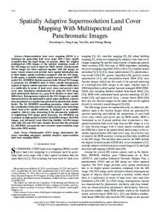
spaces. Other variants such as similarity constraints [13], DCTdomain priors [14], and local pixel structure constraint [15] have also been considered for better reconstruction performance. These NE based approaches yield decent visual image quality in noise-free scenarios. Since they eliminate overfitting by selecting k compact neighbors (or a single manifold), when the input face images are contaminated by noise, they could be embedded into multi-manifolds, leading to oversampled manifolds and hence performance degradation. SR based approaches integrate various regularization terms to handle the under- or over-fitting problem in representation schemes. The goal is to learn better a priori knowledge from the input images. Yang et al. [16] used raw patches in an over-complete dictionary while assuming invariant HR and LR sparse representation weights. Ma et al. [17], [18], [19] proposed a least-square representation based hallucination method to extract the prior from the same facial position patches. Jung et al. [20] utilized sparse representation based superresolution to avoid over-fitting in position-based hallucination. Jiang et al. [21] argued that locality-constrained representation introduces both locality and sparsity. Wang et al. [22] introduced an adaptive regularization term (in lq norm) to enhance the sparsity of representation coefficients. Gao et al. [23] used dual-low-rank representation on reconstruction error and representation coefficients for effectively hallucinating. The above representation based approaches, assume that the inputs and primary dictionary atoms lie in one subspace and use either sparsity regularization [16], [20], [22], [24] or locality regularization [10], [11], [21], [14], [25] to discover a priori from sample space. However, these approaches do not exploit the structural prior from multi-subspace (multimanifold) which include smooth patches, texture patches, edge patches etc. When the inputs are near the intersection of multiple subspaces, they could be selected into wrong subspace, leading to performance degradation. As illustrated in Fig.1, where it is assumed that the space spanned by the dictionary atoms has two subspaces: subspace 1 (red dots) of smooth patches and subspace 2 (blue triangles) of texture patches. In Fig.1 (a), sparsity regularization focuses on randomly selecting a few atoms (e.g., only 3 atoms) to represent the test sample, and these three atoms are randomly chosen from both subspace 1 and subspace 2. However, random selection leads to unstable solution that similar inputs may have totaly different selected dictionary atoms in sparse representation. Whereas locality regularization seeks a few distance-inducing nearest atoms to represent the test sample, as shown in Fig.1 (b), when one smooth patch is selected to synthesize testing texture patch, it may degrade the texture of output patch. From above observation, there is no guarantee that the selected atoms and test samples will share similar structural patterns while lying in the same subspace. As illustrated in Fig. 1 (c), one optimized selection of atoms to perfectly represent the test sample is choosing a few (sparsity), nearest (locality) and subspace consistent (low-rank) atoms. Candes et al. [26] proved a stable subspace that provides structure constraint and against noise and outliers can be perfectly recovered by low-rank minimization. After that, low-rank representation has been used in unsupervised sub-

Fig. 1. Different regularization terms select different dictionary atoms to represent the test sample. Shapes in red indicate selected atoms.

space clustering to classify data into different subspace with stable structural constraints [27], [28], [29], [30], achieving promising results in various vision-based tasks. Inspired by these work, we propose a novel approach based on localityconstrained low-rank representation (LLR) to reveal the intrinsic structures of multi-subspace from samples. The aim of LLR is to exploit the low-rank (subspace constraint) and manifold structures (locality constraint) to boost the reconstruction performance. We introduce a low-rank regularization term into locality-constrained representation scheme to simultaneously exploit multi-manifold structural and local priors from sample space. By imposing a low-rank constraint on the dictionary atoms that lie in the vicinity of the input patches, we are able to cluster patches into nearly stable independent linear subspaces for better exploiting subspace structural prior. The main contributions of this paper are summarized as following: 1) We develop a novel low-rank representation framework with a locality constraint, termed LLR, to exploit the subspace structural prior from sample space for face super-resolution. 2) LLR extends neighbor embedding based approaches from a single smooth manifold space to multiple manifold spaces without the need of fine tuning the number of embedding neighbors. 3) LLR can be viewed as a generalization of representation based methods i.e. least squares representation [17], sparse representation [16], and locality-constrained representation [21]. Furthermore, the multi-layered nature of LLR leads to its better performance for super-resolution. We extend our preliminary work [31] with more technical details of LLR, including its multi-layered nature that is partially responsible for its superb performance, and analysis on the low-rank, locality, accuracy, and robustness properties of LLR. The rest of this paper is organized as follows. Section II gives the notation and background of representation schemes. Section III introduces our proposed LLR based hallucination as well as its optimization. Section IV addresses the low-rank and sparsity properties of LLR and analyzes LLR’s accuracy and robustness capabilities. Experimental results are presented in Section V and conclusion is drawn in Section VI. II. R ELATED WORK In representation based super-resolution scheme, each input image patch is represented as a linear combination of atoms from a well-designed compact dictionary (e.g., of wavelet bases) or an over-complete sparse representation dictionary. Given an l-dimensional testing sample y ∈ Rl×1 and a p-atom

2169-3536 (c) 2016 IEEE. Translations and content mining are permitted for academic research only. Personal use is also permitted, but republication/redistribution requires IEEE permission. See http://www.ieee.org/publications_standards/publications/rights/index.html for more information.

This article has been accepted for publication in a future issue of this journal, but has not been fully edited. Content may change prior to final publication. Citation information: DOI 10.1109/ACCESS.2017.2717963, IEEE Access 3

dictionary Φ ∈ Rl×p , the linear representation coefficients can be generally formulated in a Lagrangian form as α = arg min{||y − Φα||22 + λΩ(α)}, α

(1)

where α ∈ Rp×1 is the representation coefficient vector, whose entries are weights signifying contribution of associated atoms in the dictionary. Different regularization terms yield different results by varying the prior function Ω(α).

low-rank constraint on A will cluster the testing sample yi ’s into intrinsic subspaces. In face hallucination, if we assume that face images from a person with varying illumination, expression or even corruption lie in a linear subspace, then the subspace of clean images which represent intrinsic structure information should have low rank, thus in this low-rank subspace, features are robust to noise or outliers. III. P ROPOSED M ETHOD

A. Sparse Representation Mathematically, a sparse coding of y can be obtained by solving an `0 -minimization problem with α = arg min ||α||0 s.t. ||y − Φα||22 ≤ ε, where || · ||0 is a pseudo α norm that counts the number of non-zero entries in α and ε a small constant controlling the approximation error. It is well known that `0 -minimization is NP hard, thus itPis often relaxed p to a convex `1 -minimization with ||α||1 = i=1 |αi |. Then sparse representation can be formulated as 2

α = arg min{||y − Φα||2 +λ||α||1 }, α

(2)

where λ is the regularization parameter. Iteration thresholding [32] and Bregman split algorithms [33] can be employed to efficiently solve `1 -minimization problems. B. Locality-constrained Representation Locality-constrained representation (LCR) introduces a manifold regularization on coding vector. The objective function is formulated as 2

α = arg min{||y − Φα||22 + λ||d ⊗ α||2 } s.t. 1T α = 1, (3) α

where ⊗ is the element-wise product operator and d = [d1 , d2 , ..., dp ]T a locality metric vector, with each element di describing the similarity between the input patch y and the i-th atom φi in the dictionary, the constraint 1T α = 1 ensures shift-invariance of LCR, and λ > 0 is a regularization parameter. With local smooth sparsity [34], LCR leads to superior reconstruction. Moreover, an analytical solution to (3) can be easily obtained by solving a regularized least square problem [21]. C. Low-rank Representation Recently, low-rank representation (LRR) has been widely used in data segmentation and classification tasks [27], [29], [28]. Given a testing sample matrix Y = [y1 , y2 , ...yN ] ∈ Rl×N , where each column vector yi represents an ldimensional testing sample and N is the number of samples, LRR seeks a low-rank coefficient matrix A = [α1 , α2 , ...αN ] ∈ Rp×N that is the solution to arg min ||A||∗ s.t. Y = ΦA, A

(4)

Pmin{p,N } where Φ is the dictionary, ||A||∗ = σi denotes i=1 nuclear norm which relaxes the low-rank optimization [27] to a convex problem, and σi ’s are the singular values of A. Each column vector αi provides a representation of the input sample yi using atoms of the dictionary Φ. As a result, the

A. Locality-constrained Low-rank Representation LCR introduces a local manifold constraint via a similarity metric between the input patch and dictionary atoms to reveal prior information from nearest atoms in the Euclidean distance. However, locality constraint ignores the subspace structural prior that input images and dictionary atoms lie in a subspace with structure similarity. Moreover, when the input patch is corrupted by noise, Euclidean pixel-wised similarity metric may fail to recover the intrinsic manifold. In order to rectify these shortcomings, we propose a locality-constrained low-rank representation (LLR) to exploit intrinsic subspace structural priors. The idea of LLR on atom selection is illustrated in Fig. 1 (c). Whereas SR favors sparsity and ignores local manifold priors and LCR emphasizes nearest atoms in the subspace, LLR discovers both intrinsic subspace structural and local manifold prior. The idea of LLR on atom selection is illustrated in Fig. 3. Whereas SR favors sparsity and ignores local manifold priors and LCR emphasizes nearest atoms in the subspace, LLR balances both local manifold and intrinsic structural priors. In Section IV-A, we show that both SR- and LCR-based approaches can be treated as special cases of LLR. In order to reveal intrinsic subspace structures, we cluster the input patch into a low-rank subspace with the most similar dictionary atoms. Inspired by TraceLasso [35], [36], [30], we introduce a low-rank regularization term: ||Φdiag(α)||∗ which provides subspace structural constraint to further constrain the LCR objective function (3) as arg min{||y − Φα||22 + λ||Φdiag(α)||∗ +β||d ⊗ α||22 }, (5) α

where α is again the low-rank coding vector, λ and β are balancing parameters for controlling contributions from low||y−φi ||22 ) rank and locality regularization terms, and di = exp( σ is the locality metric, with σ being a constant that adjusts the speed of weight decay. For the sake of robustness, we normalize di to a fractional number between 0 to 1. Note that nuclear norm in (5) is always used as a convex substitute for rank operation. The columns of matrix Φdiag(α) represent the weighted vectors to reconstruct the input patch. Rank minimization of this matrix amounts to selecting the most accurate dictionary atoms to reconstruct patch y against noise. The columns of matrix Φdiag(α) represent the weighted vectors to reconstruct the input patch. Rank minimization of this matrix amounts to selecting the most accurate dictionary atoms to reconstruct patch y against noise. As shown in Fig. 2, suppose dictionary Φ is a full rank matrix (rank(Φ) = 6), LLR representation

2169-3536 (c) 2016 IEEE. Translations and content mining are permitted for academic research only. Personal use is also permitted, but republication/redistribution requires IEEE permission. See http://www.ieee.org/publications_standards/publications/rights/index.html for more information.

This article has been accepted for publication in a future issue of this journal, but has not been fully edited. Content may change prior to final publication. Citation information: DOI 10.1109/ACCESS.2017.2717963, IEEE Access 4

Fig. 2. Subspace structural constraint term Φdiag(α) is low-rank. Zero elements from α shrink Φdiag(α) into low-rank.

coefficient α = [0.3, 0.1, 0, 0, 0, 0.6]T , then subspace structural constraint matrix Φdiag(α) only contains 3 non-zero columns to represent input patch y, zero elements in α multiply corresponding dictionary columns, thus these columns in Φdiag(α) are all transferred into zeros (white columns in Fig. 2), then rank of subspace structural constraint matrix (rank(Φdiag(α)) = 3) is lower than rank of dictionary. For visual comparison of above algorithms how to select atoms, as shown in Fig. 3, we display 8 largest representation weights relevant atoms from three regularization schemes, LLR candidate atoms (first two rows) obviously have similar structure, the red boxes are atoms with different pattern indicate missing-matched pathes, the second and third columns of SR obviously have different texture pattern with input pathes, some totally different direction patterns (fifth and seventh columns of first input patch, second and fourth columns of second input patch) are chosen by LCR. It confirms that subspace structural constraint is more essential than sparsity and locality for obtaining better structural priors from the dictionary atoms.

where tr(·) is the trace operator, k·kF the Frobenius norm, ∆ the Lagrange multiplier, µ the penalty parameter, and λ and β parameters for balancing different regularization terms. The first step of ADMM is to optimize the low-rank matrix Λ while fixing α (and other variables). As in [37], this is done by formulating the optimization problem of 1 λ arg min{ ||Λ||∗ + ||Λ − G||2F }, Λ µ 2

(8)

T where G = Φdiag(α) + ∆ be the SVD µ . Let G = U ΣV decomposition of G, then the solution to (8) is given by softthresholding the singular values of G, leading to [28]

Λ∗ = U S λ (Σ)V T ,

(9)

µ

where S λ (Σ) = max(0, Σ − µλ ). µ The second step of ADMM is to fix Λ in (7) at the optimal low-rank matrix Λ∗ in (9) while optimizing the representation vector α via arg min{||y − Φα||22 + β||d ⊗ α||22 α µ +tr(∆T(Φdiag(α)−Λ∗ ))+ ||Φdiag(α)−Λ∗ ||2F }.(10) 2 The above problem can be reformulated in Frobenius norm as arg min{||y − Φα||22 + β||d ⊗ α||22 α

1 ∆ + ||Λ∗ −(Φdiag(α)+ )||2F }, 2 µ

(11)

where α appears in both a vector form and a matrix form diag(α). It is in general not easy to directly perform matrix optimization. However, since the objective function of (11) is in quadratic form, we can treat α and diag(α) as two separate variables, and minimization of such an objective function is achieved when its partial derivatives with respect to both variables are zero at the same time. We thus break the problem in (11) into two sub-problems: arg min{||y − Φα||22 + β||diag(d)α||22 } α

Fig. 3. Visual dictionary atoms selected by different regularization schemes. We show the 61-st and 121-st patches from the testing image in first column of each subfigure, the following 8 columns are the atoms with 8 largest representation weights. The red boxed atoms are obviously different with pattern of input patches.

and arg min {||Λ∗ −(Φdiag(α)+ diag(α)

∆ 2 )|| }. µ F

The first one can be solved by linearly constrained leastsquares [34] with solution

B. Optimization We rewrite the optimization problem of (5) as

(ΦT Φ + βdiag(d)T diag(d))α = ΦT y,

arg min{||y − Φα||22 + λ||Λ||∗ +β||d ⊗ α||22 } α,Λ

s.t. Λ = Φdiag(α)

(6)

and solve it by the alternating direction method of multiplier (ADMM) with the following augmented Lagrange function [29] arg min{||y − Φα||22 + λ||Λ||∗ +β||d ⊗ α||22 α,Λ

µ +tr(∆T(Φdiag(α)−Λ))+ ||Φdiag(α)−Λ||2F }, (7) 2

and the second one has analytical solution µΦT Φdiag(α) = µΦT Λ∗ − ΦT ∆. Noting that diag(α)1T = α, we combine the above two solutions into one, yielding α∗

= (ΦT Φ + βdiag(d)T diag(d) + µΦT Φ)−1 (ΦT y + µΦT Λ∗ 1T − ΦT ∆1T ).

(12)

2169-3536 (c) 2016 IEEE. Translations and content mining are permitted for academic research only. Personal use is also permitted, but republication/redistribution requires IEEE permission. See http://www.ieee.org/publications_standards/publications/rights/index.html for more information.

This article has been accepted for publication in a future issue of this journal, but has not been fully edited. Content may change prior to final publication. Citation information: DOI 10.1109/ACCESS.2017.2717963, IEEE Access 5

Finally, the Lagrange multiplier ∆ and penalty parameter µ are updated as follows [28] ∆ ← ∆+µ(Φdiag(α∗ ) − Λ∗ ), µ ← min(ρµ, µ),

(13)

where ρ is a constant that adjusts the speed of updating µ. The resulting ADMM algorithm for solving our LLR problem is summarized in Algorithm 1. Algorithm 1 ADMM algorithm for solving LLR Require: Input image y, pre-learned dictionary Φ, and the balance parameters λ and β; Ensure: Initialize α = ∆ = Λ = 0, ρ = 5, µ = 106 , ε = 10−8 ; 1: Step1: update Λ according to (9) while fixing others; 2: Step2: update α according to (12) while fixing others; 3: Update ∆ and µ according to (13); 4: Check for convergence ||Φdiag(α) − Z||∞ > ε Go to step 1; 5: Output the LLR coding coefficient vector α.

C. Face super-resolution via LLR We utilize LLR to improve the reconstruction performance of patch-based face hallucination algorithm. In patch-based face hallucination scenario, both training and testing images are divided into patches by position. Given an LR face image Y ∈ Rm×n , the goal of face super-resolution is to generate an HR image X ∈ Rtm×tn with a scale factor t. The √ image √ Y is divided into a set of overlapping patches of size l × l with overlapped pixels. Then the resulting patches are reshaped into column-vector in lexicological order and sorted as vector yi ∈ Rl×1 , where i ∈ [1, b] indicates the index of position patch . Respectively, we prepare p HR database images with size of tm × tn pixels and LR ones with size of m × n in same order as the training database. For i-th patch, all p patch vectors are combined to form a pair of coupled HR and LR dictionaries 2 as Hi ∈ Rt l×p and Li ∈ Rl×p , where p is the number of dictionary atoms, i represents the patch index. The position patch with index i is used to super-resolve the LR position patch yi . This setup is in line with the position-patch based method published in [21]. For input patch yi , corresponding representation weights can be solved by

Fig. 4. The outline of multi-layer LLR based face hallucination. The green arrows indicate dictionary updating phase and red arrows indicate representation weights updating phase.

D. Multi-layer LLR enhancement for face super-resolution Inspired by deep learning [38], and multi-layer superresolution [11] approaches, we cascade multiple layers of LLR to further boost the performance. As shown in Fig. 4, dictionaries and representation weights are alternately updated in each layer, then results from the previous layer are fed into next layer as input. Updating the weights: Without loss of generalization, we define m as the number of layers. Thus, for the m-th layer, the weights of i-th position patch can be generally formulated in the following Lagrangian form: (m)

αi

(m−1)

= arg min {||Xi (m) αi

(m)

λ||Li

(m)

diag(αi

(m)

− Li

(m)

)||∗ +β||di

(m) 2 ||2

αi

+

(m) 2 ||2 },

⊗ αi

(16)

(0)

it is worth to notice that Xi = yi . Thus, based on manifold consistency assumption, the corresponding i-th underlying HR (m) patch Xi are rendered by (m)

Xi

(m)

= Hi

(m)

αi

.

(17)

Updating next layer dictionary: Once getting the reconstructed HR patches from previous layer, we update the next layer LR dictionary with LLR by Leave-one-out strategy. Each time we take one image from training database to hallucinate, all the rest of training images are used as dictionary atoms, a new LR dictionary is updated after traversing the whole αi = arg min{||yi −Li αi ||22 +λ||Li diag(αi )||∗ +β||di ⊗αi ||22 }, datebase. Once LR dictionary updating is done, atoms in αi (14) updated dictionary and original HR dictionary become more with support of LR dictionary Li . Thus the latent HR image consistent, in that the LR and HR weights get more coupled patch is rendered with isometric weights by Xi = Hi αi . as well. Furthermore, all latent HR patch Xi s are stitched together to Two, three and four layers LLR are verified to signifiform a whole HR image by cantly improve the super-resolution performance. However, more layers cost more computing time, as a tradeoff between b X X = arg min{ ||Ri X − Hi αi ||22 }, (15) time and performance, we only set m = 2 to reveal the X effect of multi-layer LLR in the experiments. The face superi=1 resolution algorithm via multi-layer LLR can be summarized where Ri represents an operation matrix that extracts patch in Algorithm 2: Xi from image X at i-th position. 2169-3536 (c) 2016 IEEE. Translations and content mining are permitted for academic research only. Personal use is also permitted, but republication/redistribution requires IEEE permission. See http://www.ieee.org/publications_standards/publications/rights/index.html for more information.

This article has been accepted for publication in a future issue of this journal, but has not been fully edited. Content may change prior to final publication. Citation information: DOI 10.1109/ACCESS.2017.2717963, IEEE Access 6

Algorithm 2 Face super-resolution via multi-layer LLR Require: LR testing image Y , Training set {Hi }b1 and {Li }b1 , patch size l , scale factor t , regularization parameter λ and β, layer number m. Ensure: HR hallucinated face image X (m) 1: INITILIZATION Divide each training images and the LR input image into p patches by location of face images. 2: For each layer: j = 1 to m. 3: For patch yi : i = 1 to b. (j) 4: Calculate the optimal weight vector αi for LR input (j) patch with LR dictionary Li by formulate (16) in the first layer. (j) 5: Construct the HR patch Xi by formulate (17) as the input of second layer. (j+1) (j+1) 6: Update the second layer dictionaries Li and Hi . 7: End for i 8: End for j 9: Integrate b reconstructed HR patches into the original position by formulate (15) and generate the final output X (m) .

IV. L OW- RANK ,

ACCURACY AND ROBUSTNESS OF

LLR

Why low-rank enhances the performance of face hallucination method? The reason is justified in this section, first, we prove that low-rank is equivalent to sparsity in diagonal matrix, then check the low-rank and locality of different representations (e.g. LLR, LCR, SR and LSR) through qualitative and quantitative analysis, moreover, we analyze the accuracy and robustness of LLR in noise scenario. From both theory and experiments, simulation results verify the validity of LLR. A. Low-rank and locality 1) Low-rank and sparsity: From the perspective of matrix, the sparsity of matrix is always known as low-rank. so we here investigate sparsity of representation coefficients instead of low-rank. Proposition 1: If α ∈ Rp×1 , then rank(diag(α)) = ||α||0 . T For a vector α= [α1 ,α2 ,...αp ] ∈ Rp×1 , p is the length of this vector. Then define a diagonal matrix A ∈ Rp×p whose diagonal elements aii come from vector α , thus   a11 0 0 0  0 a22 0 0    A= (18) . ..  0 . 0 0  0

0

0

app

For diagonal matrix A, when i 6= j, ai,j = 0, if i = j, then aij = αi , if αi = 0, the column or row contains this aij can be eliminated during rank computing, so rank(A) = ||α||0 .

(19)

As we know, `0 -norm indicates the number of non-zero elements in vector α, so the rank of diagonal matrix is equal to the sparsity of diagonal vector. In order to check rank of the representation coefficients for different approaches (e.g. LCR-, SR-, LSR- and LLR-based approaches), we use sparsity of the vector to

replace the rank measure. For quantitative analysis, we use representation coefficients from simulation experimental section, details of configuration of experiments are the same with sectionV-A. We plot the concatenated optimal weight vector c of different representation methods. The optimal weight c is formed by concatenating the optimal weight vector of each patch of all 40 test face images. c = [c1 , c2 , ...cn ], n = (the number of test f ace images) × (the length of the optimal weights) × (the number of position patches). Furthermore, we quantitatively evaluate the sparsity measure of different representation-based approaches. Hoyer Measure (HM) index is a normalized version of the `1 /`2 ratio which is widely used to measure the sparsity of a given signal [39]. HM index is normalized and assumed to have values between 0 and 1 for any vector1 . HM index is defined as: √ n − l1 /l2 , (20) HM (c) = √ n−1 pPn Pn 2 where, l1 = i=1 |ci |, l2 = i=1 ci represent `1 -norm and `2 -norm of c. TABLE I H OYER M EASURE (HM) INDEX FOR DIFFERENT REPRESENTATION METHODS . Methods Hoyer Measure

LLR 0.6773

LCR 0.5908

SR 0.8106

LSR 0.3043

Table1 gives HM index results of four different representation methods. It indicates that SR method achieved the sparest representation, and LSR method gets least sparse solution. Comparing to LCR, LLR improves the HM index by 14.6%. HM index of LLR is almost two times larger than LSR based method. Comparing with SR based approach, HM index of LLR reduces 0.1333. However as we known, SR based method favors the solution on sparse and may cause unstable solution. So a suitable low-rank (sparsity) can improve the reconstruction performance in super-resolution. 2) Locality: In order to test the locality of different methods, we combine all the distance between every patches of all 40 test images to form a n-dimensional distance vector d, then the sorted version as ds = [ d[1] , d[2] , ..., d[n] ],

(21)

where d[1] ≤ d[2] ≤ ... ≤ d[n] , according to the sorted distance ds , we sort the concatenated weights vector c to form a new weight vector as cd = [c[1] , c[2] , ..., c[n] ].

(22)

We plot ds as x-axis and cd vectors as y-axis as shown in Fig. 5, it is obvious that with the increase of distance, weight decreases correspondingly. LSR method treats every atoms equally results in scattering weights to all atoms. While SR method concentrates on less atoms resulting larger intensity 1 HM index 0 is for the least sparse signal with all the coefficients having equal energy, and 1 is for the sparest one which has all the energy concentrated in just one coefficient.

2169-3536 (c) 2016 IEEE. Translations and content mining are permitted for academic research only. Personal use is also permitted, but republication/redistribution requires IEEE permission. See http://www.ieee.org/publications_standards/publications/rights/index.html for more information.

This article has been accepted for publication in a future issue of this journal, but has not been fully edited. Content may change prior to final publication. Citation information: DOI 10.1109/ACCESS.2017.2717963, IEEE Access 7

Fig. 5. The weight vectors of different representation approaches according to distance. From top to bottom, LCR based, LLR based, SR based and LSR based methods.

but still scatters to larger distance scale, LCR introduces locality constraint with closer distance, so the weights concentrates on small distance. Compared with these methods, our method further concentrates on more compact distance space which enhances the locality of LLR. In order to further check the locality of proposed method, we use an evaluation metric of locality called K-MeanDistance (K-MD) defined by [21]. Based on the definition of K-MD, the locality of a representation approach is measured by calculating the distance between the input LR patch and the K largest weight patches in the representation of the inference patch. Thus, the smaller K-MD value, the better locality. Fig. 6 gives the K-MD results of different representation based methods, from which we find that the average value of K-MD for LLR is smaller than all other methods (no matter what value of K (20,40,80)). Therefore, LLR captures better locality property than LCR, LSR and SR. In the same time, K-MD means of SR and LSR are much bigger than LCR and LLR, this further indicates that locality constraint plays an important role in representation schemes. Comparing with LCR, K-MD means of LLR are smaller in K=20,40 and 80 configurations, this indicates that our method enhances the locality by introducing low-rank representation regularization.

Proposition 2: If vectors αh , αl indicate HR and LR representation coefficients, the accuracy of representation coefficients defined as “acc”, then acc ∝ (αh )T αl . Suppose, X, Y as HR and LR patches, H,L as HR and LR dictionaries, intuitively, we get LR and HR representation coefficients αl and αh by equation(12). However, the observed HR image patch X is not available in super-resolution scenario, as a result, corresponding HR representation coefficient αh is also unavailable, in order to render the latent HR patch, we use observed LR patch Y to generate its αl , who replaces αh to render HR patch X. Thus a model error err = ||H(αh − αl )||22 occurs, it can be rewritten as ||H(αh − αl )||22 = (αh − αl )T H T H(αh − αl ).

(23)

For a fixed dictionary H, the error is determined by function T T f = (αh − αl )T (αh − αl ) = (αh ) αh + (αl ) αl − P T T T p (αh ) αl − (αl ) αh . As we know, αh αh = i=1 (αih )2 , Pp Pp lT l l 2 hT l h l α α = i=1 (αi ) , α α = i=1 (αi αi ), here, αi s inT dicate the i-th element in vector αs. Thus, f ∝ (−(αh ) αl ), this means reconstruction error is in inverse with the correlation function (αh )T αl . Since acc ∝ (−f ), then acc ∝ (αh )T αl , this means that a large correlation value results in a small error and improves reconstruction accuracy for superresolution. So we set the relevance in terms of correlation as accuracy metric in solution domain. For simulation, we use the original HR images to calculate the HR weights αh , then down-sampling by 4 and adding average blur to simulate the image degradation process, respective LR images can be got with the same way. To verify whether low-rank constraint promotes the accuracy of solution, boxplots of coefficients from different representation methods are listed in Fig. 7. Then it is clear that the low-rank constraint really reveals the structure information and regularizes the solution which remarkably promotes the accuracy of coefficients. It is worth to note that the value of relevance function itself does not mean anything but shows an advantage index for comparing the accuracy of representation coefficients. LLR improves the mean value by 17.4% than LCR which is the second best approach, and improves the mean value by 31.4% and 22.2% than SR and LSR based approaches. As a result, LLR enables the most accuracy solution comparing with other representation-based approaches.

Fig. 6. Histograms matrix of the K-mean distance for different representation methods. From top to bottom: K=20, K=40 and K=80. From left to right: LCR, LLR, SR and LSR approaches.

B. Accuracy In [40], sparse coding errors are minimized as accurate as possible to faithful reconstruct the original image, so it is reasonable to measure the accuracy of representation coefficients by their reconstruction error. In order to testify the accuracy of the representation coefficients, we need to analyze the reconstruction errors of LLR. In this work, we consider the relevance of HR and LR coefficients to evaluate the accuracy of representation coefficients.

Fig. 7. Boxplots of different representation based super-resolution methods. Y-axis represents the value of the correlation function which means larger value results in better accuracy for coefficients.

C. Robustness Robustness always means super-resolution performance stability in noise scenario. Especially, in real applications, noise

2169-3536 (c) 2016 IEEE. Translations and content mining are permitted for academic research only. Personal use is also permitted, but republication/redistribution requires IEEE permission. See http://www.ieee.org/publications_standards/publications/rights/index.html for more information.

This article has been accepted for publication in a future issue of this journal, but has not been fully edited. Content may change prior to final publication. Citation information: DOI 10.1109/ACCESS.2017.2717963, IEEE Access 8

may degrade the reconstruction performance seriously. In order to measure the robustness ability to input noise for different regularization terms, we check the relevance of coefficients between original noise-free images and noise contaminated images. Proposition 3: If vectors αw , αn represent noise-free and noise representation coefficients, the robustness of representation coefficients define as “rob”, then rob ∝ (αw )T αn . For simple illustration, we drop out the penalty terms keep the ordinary linear regression problem as y = Φα. Usually, we minimize the residual as α= arg min{||y − Φα||22 } with

Fig. 8. Correlation function values of different representation based face hallucination methods in noise situation.

α

closed-form solution. For a fixed dictionary Φ ∈ Rl×p , let Φ = U ΣV T as the SVD decomposition of the dictionary. Where U ∈ Rl×l and V ∈ Rp×p are orthogonal matrices and Σ ∈ Rl×p is a diagonal matrix with diagonal entries σ1 ≥ · · · ≥ σr > σr+1 = · · · = σmin{l,p} = 0 , r=rank(Φ) . Using the orthogonality of U and V we have: 2

||Φα − y||2 = ||U T (ΦV V T α − y)||22 ,

(24)

let z = V T α, recall Φ = U ΣV T , then above formulate can be rewritten as p r X X 2 2 T 2 T T −U y|| = (σ z − u y) + (uTi y) , ||Σ V α i i 2 i | {z } i=1

=z

i=r+1

(25) when zi∗ = σi , i = 1, ..., r, zi∗ = 0, i = r +1, ..., p, formulate (25) achieves the minimum value. Recall that z = V T α , since V is orthogonal, we can find that ||α||2 = ||V V T α||2 = ||V z||2 . Thus minimum norm solution of the linear least squares problem formulate (24) is given by uT i y

α∗ =V z ∗ =

r X uT y i

i=1

σi

vi .

(26)

From this formulate, when the value of σi is small, even a small error in the input image y will magnify the entry of α. So, rank operation such as singular value thresholding operation shrinks small value of σi to improve the robustness to input noise. Suppose, αw and αn denote noise-free and noise representation coefficients, similar to previous section, reconstruction error function f = (αw − αn )T (αw − αn ), then T T f ∝ (−(αw ) αn ). Since rob ∝ (−f ), then rob ∝ (αw ) αn , this means large correlation value usually results in small reconstruction error which indicates power robustness to noise. It is worth to note that the value of correlation is no related to reconstruction performance of super-resolution methods, but the relative value of correlation function indicates the ability of suppressing noise. In simulation experiments, we add gaussian noise with zero mean and standard deviation σ = 5 to simulate the input noise. As shown in Fig. 8, four different approaches are listed. With the structure information is used, both LRR and LCR achieves bigger correlation function value than regular LSR and SR methods. Furthermore, LLR has evidently larger correlation function values than LCR approach. This means LLR gets lower reconstruction errors than all the other comparing methods and indicates its robustness against input noise.

V. E XPERIMENTAL RESULTS In this section, we intensively investigate some state-ofthe-art face super-resolution algorithms and the proposed LLR and multi-LLR approaches both on simulated and realworld databases. These algorithms include Locally Linear Embedding (LLE) [10], Least Squares Representation (LSR) [17], Sparse Representation (SR) [41], Locality-constrained Representation (LCR) [21]. Especially, to the best of our knowledge, LCR is currently the best representation-based algorithm reported from face super-resolution literature. Furthermore, newest deep learning based super-resolution using convolutional neural networks (SRCNN) [38] is set as another baseline. Simulation experiments are conducted on FEI Database2 and details are provided in next subsection. In order to evaluate the objective quality of the reconstructed HR images, Peak signal-to-noise ratio (PSNR), structural similarity (SSIM)[42] index are selected as the objective metrics, and feature similarity (FSIM) [43] index is used to measure the low-level features for recognition tasks. Furthermore, noise simulation experiments and real world images experiments are conducted to verify the superiority of LLR and multi-LLR over other approaches. A. Database and Experimental Setting Simulation experiments in this paper are all conducted on the frontal images of FEI Face database [44]. This database includes 400 images of 200 individuals (100 male and 100 female) and every person has two frontal view images, one with neutral expression and the other with a smiling expression. All the facial images are previously aligned to a common template so that the pixel-wise features extracted from the corresponding images are roughly in the same positions. HR face images are cropped to size of 120 × 100 pixels. We randomly select 360 images (180 individuals) as the training database, the rest 40 images (20 individuals) as the testing database. We use average filter with size 5 × 5 to simulate point spread function (system blur), and down-sample the HR images with amplification factor 4. Then size of LR images is 30 × 25 pixels. For a fair comparison with other representative methods, we set the parameters for their best performance from their papers. HR patch size is set to 12 × 12 pixels with overlapped 8 pixels, and corresponding LR patch size is 3 × 3 pixels 2 http://fei.edu.br/

cet/facedatabase.html

2169-3536 (c) 2016 IEEE. Translations and content mining are permitted for academic research only. Personal use is also permitted, but republication/redistribution requires IEEE permission. See http://www.ieee.org/publications_standards/publications/rights/index.html for more information.

This article has been accepted for publication in a future issue of this journal, but has not been fully edited. Content may change prior to final publication. Citation information: DOI 10.1109/ACCESS.2017.2717963, IEEE Access 9

with overlapped 2 pixels. For Chang ’s neighbor embedding method, the number of neighbors is set to 100. For Yang ’s SR method, error tolerance is set to 0.001 during seeking SR optimal solution. For Jiang ’s LCR method, balance parameter is set to 0.04 for the best performance. In SRCNN, we use 320 face images as training data and 40 images as validation data and the rest as testing data to train a network. 4 pixels border is shaved to have the best performance, so that image size of output from SRCNN is 116 × 96 pixels, 109 backpropagations are set as a check point to evaluate the performance of SRCNN, training time is about 344 hours (more than 2 weeks) with GPU GTX1070. In our method, same setup is used that we use as above patch-based approaches. The input noise is simulated with Gaussian distribution with zero mean and different variances. B. Parameters Configuration In this section, we further analyze the connections between LLR and other representation based approaches. In LLR, there are two parameters: low-rank parameter λ and locality parameter β rather than one in other position-based methods. These two parameters are used to balance the different contribution of regularization terms. With different regularization parameter configurations, our method can be thought into four different cases. It is easy to see LLR can be considered as an unified framework for position-based face super-resolution methods. 1) λ = 0, β 6= 0: When λ = 0 , objective function (5) drops the low-rank constraint term ||Φdiag(α)||∗ . Then the objective function only contains locality-constrained term, so our method is equivalent to LCR based method. 2) β = 0, λ 6= 0: When β = 0, objective function (5) drops the locality constraint term ||d ⊗ α||22 . The objective function only contains low-rank constrained regularization term. We prove that rank of diagonal matrix is equivalent to l0 -norm. For function (5), as we know, the dictionary Φ is fixed in advance and with rank no more than min{l, p}. Usually, l < p, then rank(Φdiag(α)) ≤ l. However dictionary matrix Φ is fixed in advance, this means α should be l-sparse. This further indicates that low-rank regularization is a general form for sparse representation. 3) λ = 0, β = 0: When λ = 0 and β = 0 , objective function (5) only contains data error term. So the objective function degrades to a regular Least Squares problem. The proposed method is equivalent to LSR based approach. Furthermore, without regularization term, if the number of atoms (K) in dictionary (Neighbor Embedding scheme uses K-nearest neighbors patches to make up the dictionary) is a variable, then the proposed method is equivalent to LLE based approach. 4) λ 6= 0, β 6= 0: When two regularization parameter are both non-zero, it means that both low-rank and localityconstrained are applied in the reconstruction. However, how to determine these two parameters is still hard-to-deal. We carefully fine-tune the parameters by experience, from Fig. 9, PSNR, SSIM and FSIM are plotted by different λ and β. For a fixed β, vary λ until PSNR, SSIM and FSIM all achieves the peak. On the other hand, for a fixed λ, vary β.

TABLE II PARAMETERS SETTING

FOR DIFFERENT FACE SUPER - RESOLUTION METHODS WITH DIFFERENT NOISE LEVELS

Noise level σ=0 σ=5 σ=10 σ=15 σ=20

LLE K 100 100 60 50 20

λ 0 0 0 0 0

LSR λ 0 0 0 0 0

SR λ 0.001 0.0015 0.01 0.02 0.029

LCR λ 0.04 0.6 2.5 5.5 8.5

LLR λ 0.01 0.013 0.019 0.022 0.025

β 0.4 45 50 60 69

As a result, at λ = 0.01 β = 0.4 all the three measure metrics reach the peak. Table.2 gives all the parameter setting for different face super-resolution methods with different noise levels. Where for LLE-based method, K is the number of embedding patches, λ = 0. For the other methods, K = 360. In LLE and LSR based methods, they do not use regularization terms, λ set at 0. In SR-based approach, λ is the reconstruction error which controls the sparsity. In LCR, λ is locality regularization parameter uses as the best performance. For the proposed approach, λ and β increase as the noise level increases. This means that these two regularization terms play important roles in noise scenario. As we know, low-rank singular value thresholding operation shrinks small value of singular value, so λ should not be too big. C. Simulation on FEI database In this part, we conduct simulation experiments on FEI database with both noise and noise free two different configurations. As usual, we adopt the same assessment methods (PSNR, SSIM and FSIM) to measure the objective and subjective qualities of the reconstructed images with other algorithms. 1) Experiments without noise: As shown in Fig. 10, we list five facial images for comparing the subjective quality of each algorithm. For the proposed methods, we only utilize the second layer (LLR2) output as final results. We can find that our method is better than other methods in subjective quality. LLE approach suffers under-fitting, facial image has blurring effects in details of mouths and eyes. LSR approach suffers over-fitting and also lack enough detail about facial location. SR and LCR approaches have similar subjective performance, and SRCNN yields good subjective images with second best PSNR. Remarkably, our method yields more details in mouth and eye regions, which are more identical with original images. Furthermore, we list average PSNR, SSIM and FSIM of all 40 testing images in Table 3. We compare our first layer results (LLR1)with other representation based methods and list the second layer resluts (LLR2) to compare with deep learning based SRCNN approach. We bold the best and second best performance values for easy comparing. In noise-free scenario, LLR1 has average 0.20 dB higher than LCR. LLR2 has average 0.18 dB higher than SRCNN and 0.42dB higher than LCR. In the same time, LLR2 improve SSIM and FSIM by 0.0077 and 0.004 compare to the second best method SRCNN. Therefore, we can conclude that our method has better performance both in objective and subjective than stateof-the-art methods with noise free scenario.

2169-3536 (c) 2016 IEEE. Translations and content mining are permitted for academic research only. Personal use is also permitted, but republication/redistribution requires IEEE permission. See http://www.ieee.org/publications_standards/publications/rights/index.html for more information.

This article has been accepted for publication in a future issue of this journal, but has not been fully edited. Content may change prior to final publication. Citation information: DOI 10.1109/ACCESS.2017.2717963, IEEE Access 10

Fig. 9. PSNR ,SSIM and FSIM of LRR with different low-rank regularization parameter λ and locality-constrained regularization parameter β. TABLE III P ERFORMANCE COMPARISON OF DIFFERENT SUPER - RESOLUTION METHODS WITH DIFFERENT NOISE LEVELS . Methods Bicubic

LLE

LSR

SR

LCR

SRCNN

Fig. 10. Comparison of results based on different methods. From left to right: Input LR faces, Hallucination images by LLE [10], LSR [17], SR [41], LCR [21],SRCNN [38], LLR2. The last column is original HR faces.

LLR1

LLR2

Remarks 1 In noise-free scenario, although LLR1 has less PSNR than SRCNN, it still yields better SSIM and FSIM among competitors, furthermore, LLR2 further improves the performance. The reason for this is that the second layer dictionary updating overcomes the resolution gap between LR and HR. 2) Robustness against noise: In order to test the robustness of proposed methods, we conduct experiments on noise situations with zero mean Gaussian noise and standard deviation (σ) from 5, 10, 15 to 20. Average evaluation measures of all the 40 testing images are listed in table.3. During noise situation, the reconstruction qualities of all these super-resolution methods reduce when the input noise intensity increases. LSR treats all the dictionary atoms equally, when input patches contaminated by noise, intrinsic pixel-wise features and noise features are represented in the same time without discrimination. Although sparse representation has good performance in image reconstruction, when input images patches are contaminated by noise, the representation coefficients seek the sparsest atoms rather than reducing noise bias. So SR based approach does not get satisfied results in noise scenario. LLE based approach uses less dictionary atoms for coding the input patch, the embedded atoms are more related to the input patches resulting reasonable reconstruction quality. However, less embedded atoms reduce reconstruction ability

Noise level PSNR SSIM FSIM PSNR SSIM FSIM PSNR SSIM FSIM PSNR SSIM FSIM PSNR SSIM FSIM PSNR SSIM FSIM PSNR SSIM FSIM PSNR SSIM FSIM

σ=0 27.49 0.8417 0.8793 31.35 0.8974 0.9185 32.04 0.9083 0.9266 32.50 0.9142 0.9332 32.89 0.9186 0.9373 33.13 0.9188 0.9398 33.09 0.9208 0.9373 33.31 0.9265 0.9438

σ=5 26.91 0.7970 0.8593 29.71 0.8382 0.8973 28.48 0.7641 0.8594 29.73 0.8390 0.8993 30.23 0.8475 0.9083 28.27 0.7388 0.8546 30.32 0.8519 0.9161 30.58 0.8651 0.9190

σ = 10 25.60 0.6994 0.7485 27.06 0.7275 0.8515 24.36 0.5588 0.7486 27.39 0.7765 0.8704 28.29 0.8006 0.8873 23.32 0.4806 0.7111 28.39 0.8033 0.8881 28.75 0.8296 0.8983

σ = 15 24.08 0.5954 0.6559 24.79 0.6194 0.8022 21.36 0.4048 0.6560 25.80 0.7115 0.8432 27.03 0.7703 0.8726 19.80 0.3133 0.6002 27.24 0.7747 0.8740 27.58 0.8088 0.8858

σ = 20 22.61 0.5027 0.5845 23.01 0.5315 0.7591 19.11 0.2990 0.5845 24.40 0.6365 0.8103 26.06 0.7444 0.8602 17.35 0.2146 0.5216 26.33 0.7522 0.8625 26.64 0.7903 0.8750

of LLE. Manifold structure improves the discriminative ability of representation coefficients, thus LCR approach selects the nearest dictionary atoms, resulting better reconstruction performance, while noise intensity is relative large (σ ≥ 10), it is hard to distinguish noise during coding and reconstruction. Additionally, SRCNN does not achieve satisfied reconstruction performance in noise scenario, even worse than representationbased methods, because we do not add noise into the training databases. For LLR, low-rank of coefficients trap the atoms in intrinsic structure subspace, especially, LLR automatically embeds stable subspace to support reconstruction against input noise, moreover, multi-layer LLR further filters input noise layer by layer to provider better results. Consequently, the proposed methods indeed improve the reconstruction performance better than LCR and other patch-based methods and even typical deep learning based method (SRCNN). For visual comparison of different super-resolution methods in noise situations, we list several representative face images to show the subjective reconstruction image quality. As shown in Fig. 11 (σ = 10) and Fig. 12 (σ = 20). In noise situation, outputs of LSR look similar to input noise images since noise is simultaneously reconstructed as normal pixels. LLE gives better visual performance than LSR

2169-3536 (c) 2016 IEEE. Translations and content mining are permitted for academic research only. Personal use is also permitted, but republication/redistribution requires IEEE permission. See http://www.ieee.org/publications_standards/publications/rights/index.html for more information.

This article has been accepted for publication in a future issue of this journal, but has not been fully edited. Content may change prior to final publication. Citation information: DOI 10.1109/ACCESS.2017.2717963, IEEE Access 11

due to less atoms are used in reconstruction. As a prestigious method, SR based approach reconstructs images with ring effect, especially at edges of face, distortion is obvious due to unsmooth solution in noise scenario. Results from LCR seem more reliable than previous methods with less ghosting. However, block effects are still evident due to biased solution from input noise. SRCNN does not yield satisfied subjective images due to no noise in training data, the trained noise-free networks are incapable to against input noise. Comparing with all other methods, our approaches render smoother images with less block effect and more details, it testifies low-rank of representation is a robust tool to deal with noise. In the same time, multi-layer LLR reduces the noise to produce better subjective image quality layer by layer. From Fig. 12, when input noise intensity increases, the visual quality declines, however, our approach still gives satisfied outputs. These experiments prove that the proposed method achieves better performance and is more robust than other comparing face super-resolution algorithms. Remarks 2 LLR1 behaves robustness against input noise, and yields both better subjective and objective images than several representative face super-resolution algorithms, LLR2 further improves image reconstruction qualities layer by layer to clean up noise gradually. This asserts the role of low-rank during super-resolution in noise scenario: the worse noise the larger gain than other methods. The reason SRCNN does not achieve good results in noise scenario is that training data includes only clean data rather than noisy training samples. Because training data of all algorithms in this paper are the same clean version, for fair comparing, noise should not be added into training data for SRCNN. D. Real-world Experiments Furthermore, we perform two more experiments: 1). experiment on real-world scenario (CMU Frontal Face database [45]), 2). experiment on real surveillance scenario to testify our methods with real world images. Testing images from realworld setup are shown in Figs. 12 and 14.

Fig. 11. Visual comparison of different face hallucination methods with noise level σ = 10. From left to right, inputs with noise, Chang et al.’s LLE [10], Ma et al.’s LSR [17], Yang et al.’s SR [41], Jiang et al.’s LCR [21], Dong et al.’s SRCNN [38],proposed LLR approach and original HR images.

Fig. 12. Visual comparison of different face hallucination methods with noise level σ = 20 . From left to right, inputs with noise, Chang et al.’s LLE [10], Ma et al.’s LSR [17], Yang et al.’s SR [41], Jiang et al.’s LCR [21], Dong et al.’s SRCNN [38],proposed LLR approach and original HR images.

Fig. 13. Testing face images from CMU frontal face database. The red mask regions are cropped as input testing samples.

1) CMU face database experiment: We extract the testing samples from CMU Frontal Face database and align the input face images to the training database according to two center points of eyes. As shown in Fig. 13, we crop six representative face images in red boxes in their original size, then, these aligned images are normalized into 30 × 25 pixels by Bicubic interpolation. It is worth to note that, these face images are originally in LR which is different from down-sampling HR images by pre-defined degradation process in above simulation experiments. In the end, we reconstruct the HR images by different approaches and list all the results in Fig. 14. The parameters for different algorithms are fine tuned for their best performance in Table.2 according the input noise levels. Obviously, our method yields more reasonable results even the test images are drastically different with the training database and degraded by noise. As an generalization of representation based approaches, the proposed approaches yield smoother images and look more reasonable with less ghosting effect than all competitors. 2) Real surveillance camera image experiment: As shown in Fig. 15, pictures are taken by a surveillance camera with CIF-size (352 × 288 pixels) in low light situation. The red boxes parts in each images are the interested face images we wish to get. We crop the frontal face images and align with the training database with size of 30 × 25 pixels by Bicubic interpolation. Then we reconstruct the desired HR outputs by

2169-3536 (c) 2016 IEEE. Translations and content mining are permitted for academic research only. Personal use is also permitted, but republication/redistribution requires IEEE permission. See http://www.ieee.org/publications_standards/publications/rights/index.html for more information.

This article has been accepted for publication in a future issue of this journal, but has not been fully edited. Content may change prior to final publication. Citation information: DOI 10.1109/ACCESS.2017.2717963, IEEE Access 12

Fig. 16. Visual results of different face hallucination methods from real surveillance camera. From left to right, inputs face images, super-resolution images by LLE [10], LSR [17], SR [41], LCR [21], SRCNN [38], LLR approach. The last column is HR images captured by same surveillance camera with closer distance for reference.

Fig. 14. Visual results from different face hallucination methods for realworld scenario CMU frontal face database. From left to right, inputs face images, super-resolution images by LLE [10], LSR [17], SR [20], LCR [21], SRCNN [38], LLR approach.

Fig. 15. Testing pictures captured by real surveillance camera. The red mark regions are the interest faces with low illumination.

different face super-resolution methods as listed in Fig. 16. The first column images are the LR inputs cropped from real surveillance camera with visible distortion. The third column are results from LSR method, which do not reduce noise intensity but enlarging disturbance. LLE, LCR and our methods all suppress the input noise. The local manifold constraint for these methods contributes the robustness to input noise. However, due to the over- or under-fitting solution of LLE and SR methods, their visual performance suffers by obvious blocking-artifacts. Comparing with LCR method, our method yields smoother images with less blocking-artifacts effects. Obviously our approach achieves the best visual performance. It reduces most of input noise and looks more similar to HR reference images. VI. C ONCLUSION In this paper, we proposed a novel low-rank representation based face super-resolution algorithm. Rather than only focus on the locality manifold regularization, we take both advantages of low-rank and locality constraints on representation, to choose the dictionary atoms from same clusters with input patches. Experimental results shown our methods have both superior subjective and objective qualities than state-of-thearts. However, some issues are still existing which needs to be investigated in the future. • Experimental results show that the low-rank prior is useful for patch-based representation. However, low-rank

•

representations include SVD decomposition and iterative algorithms are time-consuming. Furthermore, during the singular value thresholding operator, adaptively selecting the shrinkage threshold still has space to improve. So designing an efficient low-rank representation optimization algorithm is one of our future works. Prior learned from training database is essential for representation based face super-resolution methods. However, pose, expression, illumination and noise often degrade the reconstruction quality. Similar with deep learning, deep representation framework for those seriously degraded images should also be investigated in the future works. R EFERENCES

[1] N. Wang, D. Tao, X. Gao, X. Li, and J. Li, “A comprehensive survey to face hallucination,” International Journal of Computer Vision, vol. 106, no. 1, pp. 9–30, Aug 2014. [2] E. J. Cand`es and C. Fernandez-Granda, “Towards a mathematical theory of super-resolution,” Communications on Pure and Applied Mathematics, vol. 67, no. 6, pp. 906–956, 2014. [3] X. Wang and X. Tang, “Hallucinating face by eigentransformation,” IEEE Transactions on Systems, Man, and Cybernetics, Part C (Applications and Reviews), vol. 35, no. 3, 2005. [4] K. Huang, R. Hu, Z. Han, T. Lu, J. Jiang, and F. Wang, “Face image superresolution via locality preserving projection and sparse coding,” Journal of Software, vol. 8, no. 8, 2013. [5] T. Lu, R. Hu, Z. Han, J. Jiang, and Y. Zhang, “From local representation to global face hallucination: A novel super-resolution method by nonnegative feature transformation,” in 2013 Visual Communications and Image Processing (VCIP), Nov 2013, pp. 1–6. [6] H. Zhou, J. Hu, and K. M. Lam, “Global face reconstruction for face hallucination using orthogonal canonical correlation analysis,” in 2015 Asia-Pacific Signal and Information Processing Association Annual Summit and Conference (APSIPA), Dec 2015, pp. 537–542. [7] H. Zhou, Z. Kuang, and K. Y. K. Wong, “Markov weight fields for face sketch synthesis,” in 2012 IEEE Conference on Computer Vision and Pattern Recognition (CVPR), June 2012, pp. 1091–1097. [8] H. Wang, X. Gao, K. Zhang, and J. Li, “Single-image super-resolution using active-sampling gaussian process regression,” IEEE Transactions on Image Processing, vol. 25, no. 2, pp. 935–948, Feb 2016. [9] Y. Bengio, A. Courville, and P. Vincent, “Representation learning: A review and new perspectives,” IEEE Transactions on Pattern Analysis and Machine Intelligence, vol. 35, no. 8, pp. 1798–1828, Aug 2013. [10] H. Chang, D.-Y. Yeung, and Y. Xiong, “Super-resolution through neighbor embedding,” IEEE Transactions on Systems, Man, and Cybernetics, Part C: Applications and Reviews, vol. 1, no. 3, pp. I–I, 2004. [11] J. Jiang, R. Hu, Z. Wang, and Z. Han, “Face super-resolution via multilayer locality-constrained iterative neighbor embedding and intermediate dictionary learning,” IEEE Transactions on Image Processing, vol. 23, no. 10, pp. 4220–4231, Oct 2014.

2169-3536 (c) 2016 IEEE. Translations and content mining are permitted for academic research only. Personal use is also permitted, but republication/redistribution requires IEEE permission. See http://www.ieee.org/publications_standards/publications/rights/index.html for more information.

This article has been accepted for publication in a future issue of this journal, but has not been fully edited. Content may change prior to final publication. Citation information: DOI 10.1109/ACCESS.2017.2717963, IEEE Access 13

[12] J. Jiang, R. Hu, C. Liang, Z. Han, and C. Zhang, “Face image superresolution through locality-induced support regression,” Signal Processing, vol. 103, pp. 168–183, 2014. [13] H. Li, L. Xu, and G. Liu, “Face hallucination via similarity constraints,” IEEE Signal Processing Letters, vol. 20, no. 1, pp. 19–22, Jan 2013. [14] W. Zhang and W. K. Cham, “Hallucinating face in the dct domain,” IEEE Transactions on Image Processing, vol. 20, no. 10, pp. 2769–2779, Oct 2011. [15] J. Jiang, C. Chen, J. Ma, Z. Wang, Z. Wang, and R. Hu, “Srlsp: A face image super-resolution algorithm using smooth regression with local structure prior,” IEEE Transactions on Multimedia, vol. 19, no. 1, pp. 27–40, 2017. [16] J. Yang, J. Wright, T. Huang, and Y. Ma, “Image super-resolution as sparse representation of raw image patches,” in 2008 IEEE Conference on Computer Vision and Pattern Recognition(CVPR), June 2008, pp. 1–8. [17] X. Ma, J. Zhang, and C. Qi, “Hallucinating face by position-patch,” Pattern Recognition, vol. 43, no. 6, pp. 2224–2236, 2010. [18] X. Ma, H. Q. Luong, W. Philips, H. Song, and H. Cui, “Sparse representation and position prior based face hallucination upon classified over-complete dictionaries,” Signal Processing, vol. 92, no. 9, pp. 2066 – 2074, 2012. [19] X. Ma, H. Song, and X. Qian, “Robust framework of single-frame face superresolution across head pose, facial expression, and illumination variations,” IEEE Transactions on Human-Machine Systems, vol. 45, no. 2, pp. 238–250, April 2015. [20] C. Jung, L. Jiao, B. Liu, and M. Gong, “Position-patch based face hallucination using convex optimization,” IEEE Signal Processing Letters, vol. 18, no. 6, pp. 367–370, June 2011. [21] J. Jiang, R. Hu, Z. Wang, and Z. Han, “Noise Robust Face Hallucination via Locality-Constrained Representation,” IEEE Transactions on Multimedia, vol. 16, no. 5, pp. 1268–1281, 2014. [22] Z. Wang, R. Hu, S. Wang, and J. Jiang, “Face Hallucination Via Weighted Adaptive Sparse Regularization,” IEEE Transactions on Circuits and Systems for Video Technology, vol. 24, no. 5, pp. 802–813, 2014. [23] G. Gao, X. Y. Jing, P. Huang, Q. Zhou, S. Wu, and D. Yue, “Localityconstrained double low-rank representation for effective face hallucination,” IEEE Access, vol. 4, no. 99, pp. 8775 – 8786, 2017. [24] Y. Li, C. Cai, G. Qiu, and K.-M. Lam, “Face hallucination based on sparse local-pixel structure,” Pattern Recognition, vol. 47, no. 3, pp. 1261 – 1270, 2014. [25] Y. Zhang, Y. Zhang, J. Zhang, and Q. Dai, “Ccr: Clustering and collaborative representation for fast single image super-resolution,” IEEE Transactions on Multimedia, vol. 18, no. 3, pp. 405–417, March 2016. [26] E. J. Cand`es and B. Recht, “Exact matrix completion via convex optimization,” Foundations of Computational Mathematics, vol. 9, no. 6, pp. 717–772, 2009. [27] G. Liu, Z. Lin, S. Yan, J. Sun, Y. Yu, and Y. Ma, “Robust Recovery of Subspace Structures by Low-Rank Representation,” IEEE Transactions on Pattern Analysis and Machine Intelligence, vol. 35, no. 1, pp. 171– 184, 2013. [28] K. Tang, R. Liu, Z. Su, and J. Zhang, “Structure-Constrained Low-Rank Representation,” IEEE Transactions on Neural Networks and Learning Systems, vol. 25, no. 12, pp. 2167–2179, 2014. [29] Z. Jiang, P. Guo, and L. Peng, “Locality-Constrained Low-Rank Coding for Image Classification,” in 2014 Twenty-Eighth AAAI Conference on Artificial Intelligence, June 2014, pp. 2780–2786. [30] D. Arpit, G. Srivastava, and Y. Fu, “Locality-constrained Low Rank Coding for face recognition,” in 2012 21st International Conference on Pattern Recognition (ICPR), Nov 2012, pp. 1687–1690. [31] T. Lu, Z. Xiong, Y. Wan, and W. Yang, “Face hallucination via localityconstrained low-rank representation,” in 2016 IEEE International Conference on Acoustics, Speech and Signal Processing (ICASSP), March 2016, pp. 1746–1750. [32] J. Mairal, F. Bach, J. Ponce, and G. Sapiro, “Online learning for matrix factorization and sparse coding,” J. Mach. Learn. Res., vol. 11, pp. 19– 60, Mar. 2010. [33] T. Goldstein and S. Osher, “The split bregman method for l1-regularized problems,” SIAM Journal on Imaging Sciences, vol. 2, no. 2, pp. 323– 343, 2009. [34] J. Wang, J. Yang, K. Yu, F. Lv, T. Huang, and Y. Gong, “Localityconstrained linear coding for image classification,” in 2010 IEEE Conference on Computer Vision and Pattern Recognition (CVPR), June 2010, pp. 3360–3367. [35] E. Grave, G. Obozinski, and F. R. Bach, “Trace lasso: a trace norm regularization for correlated designs,” in 2011 Twenty-Fifth Annual

[36] [37] [38] [39] [40] [41] [42]

[43] [44] [45]

Conference on Neural Information Processing Systems (NIPS), Dec 2011, pp. 2187–2195. J. Lai and X. Jiang, “Supervised trace lasso for robust face recognition,” in 2014 IEEE International Conference on Multimedia and Expo (ICME), July 2014, pp. 1–6. T. Zhang, B. Ghanem, S. Liu, C. Xu, and N. Ahuja, “Low-rank sparse coding for image classification,” in 2013 IEEE International Conference on Computer Vision (ICCV), Dec 2013, pp. 281–288. C. Dong, C. C. Loy, K. He, and X. Tang, “Image super-resolution using deep convolutional networks,” IEEE Transactions on Pattern Analysis and Machine Intelligence, vol. 38, no. 2, pp. 295–307, Feb 2016. N. Hurley and S. Rickard, “Comparing measures of sparsity,” IEEE Transactions on Information Theory, vol. 55, no. 10, pp. 4723–4741, Oct 2009. W. Dong, L. Zhang, G. Shi, and X. Li, “Nonlocally centralized sparse representation for image restoration,” IEEE Transactions on Image Processing, vol. 22, no. 4, pp. 1620–1630, April 2013. J. Yang, J. Wright, T. S. Huang, and Y. Ma, “Image super-resolution via sparse representation,” IEEE Transactions on Image Processing, vol. 19, no. 11, pp. 2861–2873, Nov 2010. Z. Wang, A. C. Bovik, H. R. Sheikh, and E. P. Simoncelli, “Image quality assessment: from error visibility to structural similarity,” IEEE Transactions on Image Processing, vol. 13, no. 4, pp. 600–612, April 2004. L. Zhang, L. Zhang, X. Mou, and D. Zhang, “Fsim: A feature similarity index for image quality assessment,” IEEE Transactions on Image Processing, vol. 20, no. 8, pp. 2378–2386, Aug 2011. C. E. Thomaz and G. A. Giraldi, “A new ranking method for principal components analysis and its application to face image analysis,” Image and Vision Computing, vol. 28, no. 6, pp. 902 – 913, 2010. H. A. Rowley, S. Baluja, and T. Kanade, “Neural network-based face detection,” IEEE Transactions on Pattern Analysis and Machine Intelligence, vol. 20, no. 1, pp. 23–38, Jan 1998.

2169-3536 (c) 2016 IEEE. Translations and content mining are permitted for academic research only. Personal use is also permitted, but republication/redistribution requires IEEE permission. See http://www.ieee.org/publications_standards/publications/rights/index.html for more information.