ROBUST IMAGE SEGMENTATION WITH MIXTURES OF STUDENT'S t-DISTRIBUTIONS. Giorgos Sfikas. Christophoros Nikou. Nikolaos Galatsanos. University ...
ROBUST IMAGE SEGMENTATION WITH MIXTURES OF STUDENT’S t-DISTRIBUTIONS Giorgos Sfikas
Christophoros Nikou
Nikolaos Galatsanos
University of Ioannina, Department of Computer Science, PO Box 1185, 45110 Ioannina, Greece, {sfikas, cnikou, galatsanos}@cs.uoi.gr ABSTRACT Gaussian mixture models have been widely used in image segmentation. However, such models are sensitive to outliers. In this paper, we consider a robust model for image segmentation based on mixtures of Student’s t-distributions which have heavier tails than Gaussian and thus are not sensitive to outliers. The t-distribution is one of the few heavy tailed probability density functions (pdf) closely related to the Gaussian, that gives tractable maximum likelihood inference via the Expectation-Maximization (EM) algorithm. Numerical experiments that demonstrate the properties of the proposed model for image segmentation are presented. Index Terms— Image segmentation, clustering, Student’s t-distribution, mixture model, EM algorithm, segmentation evaluation. 1. INTRODUCTION Image segmentation is the process of grouping image pixels based on the coherence of certain attributes such as intensity, color or texture. Many approaches have been proposed to solve the image segmentation problem. For surveys on this topic the reader may refer to [1]. In this paper, we will focus our attention to image segmentation methods based on clustering. Clustering is the process of arranging data into groups having common characteristics and is a fundamental problem in many fields of science [2]. Thus, image segmentation can be viewed a special type of clustering. Usually, in image segmentation, our data, the image pixels have spatial locations associated with them. Thus, apart from the commonality of attributes such as intensity, color or texture, commonality of location is an important characteristic of the grouping that we are seeking in image segmentation. More specifically, in this paper we will focus our attention on clustering methods based on the modeling of the probability density function (pdf) of the data via finite mixture models (FMM) [3, 4]. Modeling the pdf of data with FMM is a natural way to cluster data because it automatically provides a This work was partially supported by Interreg IIIA (Greece-Italy) grant I2101005.
1-4244-1437-7/07/$20.00 ©2007 IEEE
grouping of the data based on the components of the mixture that generated them. More specifically, FMM are based on the assumption that each datum originates from one component of the mixture according to some probability. Thus, this probability can be used to assign each datum to the component that has most likely generated it. Furthermore, the likelihood of an FMM is a rigorous measure for evaluating the clustering performance [4]. FMM based pdf modeling with Gaussian components has been used successfully in a number of applications ranging from bioinformatics [5] to image retrieval [6]. The parameters of Gaussian mixture models (GMM) can be estimated very efficiently through maximum likelihood (ML) estimation using the EM algorithm [7]. Furthermore, it can be shown that Gaussian components allow efficient representation of any pdf [4]. However, it is well known that GMM are sensitive to outliers and may lead to excessive sensitivity to small numbers of data points. The problem of providing protection against outliers in multivariate data is very difficult and increases with the dimensionality. In this paper, we apply to the image segmentation problem mixture models with Student-t pdf components. This pdf has heavier tails as compared to the exponentially decaying tails of a Gaussian [8]. Thus, each component in the mixture originates from a wider class of elliptically symmetric distributions with an additional parameter called the degrees of freedom. Hence a more robust model is used than the classical normal mixture. In the remainder of this paper, background on standard GMM is given in Section 2 and the mixture of multivariate t-distributions and the EM algorithm for parameter estimation are described in Section 3. Results on image segmentation and comparisons with the standard GMM are presented in Section 4 and conclusions are drawn in Section 5. 2. BACKGROUND ON STANDARD GAUSSIAN MIXTURE MODELS Let X denote the vector of features representing an image spatial location (pixel). The GMM assumes that the pdf of
I - 273
ICIP 2007
the observation x is expressed by φ(x; Ω) =
K �
πi f (x; μi , Σi )
(1)
i=1
where Ω is the mixture parameter set Ω = [Ω1 , Ω2 , ..., ΩK ] with Ωi = (πi , μi , Σi ). For the mixing proportions of the ith component πi , we have that K �
0 ≤ πi ≤ 1, i = 1, 2, ..., K,
πi = 1
(2)
i=1
For each component of the model in (1), the Gaussian pdf is expressed by f (x; μi , Σi ) =
1 d 1 (2π)− 2 |Σi |− 2
1
exp− 2 (x−μi )
T
Σ−1 i (x−μi )
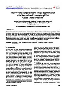
Integrating out the weights from the joint density leads to the density function of the marginal distribution: � −1 � |Σ| 2 Γ ν+d 2 (4) p(x; μ, Σ, ν) = �ν � ν+d d −1 (πν) 2 Γ 2 [1 + ν δ(x, μ; Σ)] 2 where δ(x, μ; Σ) = (x − μ)T Σ−1 (x − μ) is the Mahalanobis squared distance and Γ is the Gamma function. It can be shown that for ν → ∞ the Student’s t-distribution tends to a Gaussian distribution with covariance Σ. Also, if ν > 1, μ is the mean of X and if ν > 2, ν(ν − 2)−1 Σ is the covariance matrix of X. Therefore, the family of t-distributions provides a heavy-tailed alternative to the normal family with mean μ and covariance matrix that is equal to a scalar multiple of Σ, if ν > 2 (fig. 1).
(3)
where d is the dimensionality of the vector (e.g. intensity, location, texture features) and μi , Σi are the mean vector and covariance matrix respectively. Training of a GMM, or in other words finding its ML solution, can be performed using the EM algorithm [7]. The EM algorithm is a well-known numerical method used in a variety of ML problems. In the case of a GMM, each image pixel x, is associated with a binary hidden variable z of dimension K, whose k th component has a value of 1 if the observation (i.e. the pixel) was produced by that component and is zero otherwise. In the E-step of the algorithm, the expected value of the hidden variables conditioned on the observation is computed. These expected values give the probabilities that a given datum originates from a different component of the mixture. Thus, they provide a means for segmenting the data. In the M-step, the model parameters (mean, covariance and mixing proportions) are computed by maximizing the log-likelihood of the complete data (hidden variables and observations). This scheme is repeated iteratively until convergence is achieved.
Fig. 1. The Student’s t-distribution for various degrees of freedom. As ν → ∞ the distribution tends to a Gaussian. For small values of ν the distribution has heavier tails than a Gaussian. A Student’s t-distribution mixture model (SMM) may also be trained using the EM algorithm [8]. A K-component mixture of t-distributions is given by φ(x, Ψ) =
3. MIXTURE OF STUDENT’S t-DISTRIBUTIONS AND THE EM ALGORITHM
K �
πi p(x; μi , Σi , νi )
(5)
i=1
A d-dimensional random variable X follows a multivariate t-distribution with mean μ, positive definite, symmetric and real d × d covariance matrix Σ and has ν ∈ [0, ∞) degrees of freedom when, given the weight u, the variable X has the multivariate normal distribution with mean μ and covariance Σ/u: X|μ, Σ, ν, u ∼ N (μ, Σ/u), and the weight u follows a Gamma distribution parameterized by ν: u ∼ Gamma(ν/2, ν/2).
where x = (x1 , ..., xN )T denotes the observed-data vector and Ψ = (π1 , ..., πK , μ1 , ..., μK , Σ1 , ..., ΣK , ν1 , ..., νK )T . (6) are the parameters of the components of the mixture. Consider now the complete data vector xc = (x1 , ...xN , z1 , ..., zN , u1 , ..., uN )T
(7)
where z1 , ..., zN are the component-label vectors and zij = (zj )i is either one or zero, according to whether the observation xj is generated or not by the ith component. In the light
I - 274
of the definition of the t-distribution, it is convenient to view that the observed data augmented by the zj , j = 1, ..., N are still incomplete because the component covariance matrices depend on the degrees of freedom. This is the reason that the complete-data vector also includes the additional missing data u1 , ..., uN . Thus, the E-step on the (t + 1)th iteration of the EM algorithm requires the calculation of the posterior probability that the datum xj belongs to the ith component of the mixture: t+1 = zij
πit p(xj ; μti , Σti , νit ) K � t p(xj ; μtm , Σtm , νm )
as well as the expectation of the weights for each observation: νit
νit + d + δ(xj , μti ; Σti )
(9)
Maximizing the log-likelihood of the complete data provides the update equations of the respective mixture model parameters: N �
πit+1
t t zij uij xj N � 1 j=1 t+1 t = z , μi = N , N j=1 ij � t t zij uij
(10)
j=1 N �
Σt+1 i
=
t t zij uij (xj
−
μt+1 )(xj i
−
D(x, μ) = .
(11)
t+1 zij
j=1
The degrees of freedom for each component are computed as the solution to the equation: � t+1 � � t � � t+1 � νi νi + d νi −ψ + 1 − log + log 2 2 2 N �
+
t zij (log utij − utij )
j=1 N �
� +ψ
t zij
νit + d 2
K=3 23 20 23 26 19
K=5 17 19 17 15 15
K=7 24 21 18 17 16
the feature vector are the Lab color coordinates, the next three components are texture descriptors, namely, the polarity, the anisotropy and the contrast as described in [9] and the remaining two coordinates are the horizontal and vertical pixel locations. Prior to model training, each feature vector component was separately normalized to ensure that no feature dominates the others. In order to evaluate the proposed segmentation scheme and compare it to GMM segmentations we compute a quantization error for 30 images provided by the Berkeley image segmentation data base [10]. The quantization error, for each pixel location, is defined as the distance between the image feature and the mean of the mixture component that generated the measure (i.e. the component with the larger mixing proportion). This p-norme distance, between a d-dimensional feature vector x and the mean vector μ is defined as
μt+1 )T i
j=1 N �
Noise type noise free uniform 20 dB uniform 14 dB uniform 7 dB salt pepper 10%
(8)
m=1
ut+1 ij =
Table 1. Number of images (over 30) where the SMM provides lower quantization error than the GMM for p = 1.2.
� =0
(12)
j=1 ∂(lnΓ(x)) ∂x
where ψ(x) = is the digamma function. A detailed derivation of the EM algorithm for Student’s t-mixtures is presented in [8].
� d �
� p1 (xi − μi )p
(13)
i=1
We have experimented with different values of p, namely 0.7, 1.2 and 2 (Euclidean distance). It is well known that norms close to 1 measure a quantization error that better corresponds to human perceptual characteristics. These experiments were performed by degrading the images by uniform and salt-andpepper noise of varying strength. Also, the predefined number of kernels varied (K = 3, 5, 7). Let us also notice that the experiments were performed using a variation of the standard EM algorithm, called Greedy EM [11] providing a segmentation result independent of the model initialization. The performance of the model is presented in table 1. A comparison is shown in table 2 where one can see that the SMM has a slight yet better performance than the GMM. Some segmentation results are depicted in fig. 2 and 3 where it can be observed that SMM provide smoother segmentations than the standard GMM. 5. CONCLUSION
4. EXPERIMENTAL RESULTS In this paper, we employed an 8-dimensional vector as a feature for each image pixel [9]. The first three components of
We have presented a methodology for image segmentation based on mixtures of Student’s t-distributions. The model can account for outliers values and thus provides smoother
I - 275
Table 2. Quantization error statistics for 30 images of the Berkeley segmentation data base for all the configurations of the uniform noise (see table 1).
segmentations than the standard GMM. However, important issues for mixture based clustering still need to be addressed. Such issues are how the number of model components can be selected automatically and which features should be used. These are open questions and are subject of current research.
K=3 K=5 K=7 GMM SMM GMM SMM GMM SMM p = 0.7 mean 11.54 11.54 10.27 10.23 9.59 9.51 s. d. 0.85 0.92 0.87 0.89 0.88 0.92 p = 1.2 mean 3.85 3.83 3.48 3.47 3.27 3.25 s. d. 0.24 0.25 0.25 0.26 0.27 0.28 p = 2.0 mean 2.26 2.25 2.07 2.07 1.96 1.96 s. d. 0.12 0.13 0.14 0.14 0.15 0.15
6. REFERENCES [1] N. Pal and S. Pal, “A review of image segmentation techniques,” Pattern Recognition, vol. 26, pp. 1277– 1294, 1993. [2] R. Xu and D. Wunsch II, “Survey of clustering algorithms,” IEEE Transactions on Neural Networks, vol. 16, no. 3, pp. 645–678, 2005. [3] C. M. Bishop, Pattern Recognition and Machine Learning, Springer, 2006. [4] G. McLachlan, Finite mixture models, Interscience, 2000.
Original
GMM
Wiley-
[5] K. Blekas, A. Likas, N. Galatsanos, and I. Lagaris, “A spatially constrained mixture model for image segmentation,” IEEE Transactions on Neural Networks, vol. 16, no. 2, pp. 494–498, 2005.
SMM
[6] H. Greenspan, G. Dvir, and Y. Rubner, “Contextdependent segmentation and matching in image databases,” Computer Vision and Image Understanding, vol. 93, no. 1, pp. 86–109, 2004. [7] P. Dempster, N. M. Laird, and D. B. Rubin, “Maximum likelihood from incomplete data via EM algorithm,” Journal of the Royal Statistical Society, vol. 39, no. 1, pp. 1–38, 1977. [8] D. Peel and G. J. McLachlan, “Robust mixture modeling using the t-distribution,” Statistics and Computing, vol. 10, pp. 339–348, 2000. Fig. 2. Segmentation examples using the GMM and the SMM methods for K = 5 components.
Original
GMM
SMM
[9] C. Carson, S. Belongie, H. Greenspan, and J. Malik, “Blobworld: image segmentation using expectationmaximization and its application to image querying,” IEEE Transactions on Pattern Analysis and Machine Intelligence, vol. 24, no. 8, pp. 1026–1038, 2002. [10] D. Martin, C. Fowlkes, D. Tal, and J. Malik, “A database of human segmented natural images and its application to evaluating segmentation algorithms and measuring ecological statistics,” in Proceedings of the 8th International Conference one Computer Vision, July 2001, vol. 2, pp. 416–423.
Fig. 3. Segmentation of a MRI brain image into K = 3 classes (white matter, grey matter and cerebrospinal fluid).
[11] N. Vlassis and A. Likas, “A greedy EM algorithm for Gaussian mixture learning,” Neural Processing Letters, vol. 15, pp. 77–87, 2002.
I - 276