Robust Mapping of Process Networks to Many-Core Systems using Bio-Inspired Design Centering Gerald Hempel, Andr´es Goens, Jeronimo Castrillon
Josefine Asmus, Ivo F. Sbalzarini
Chair of Scientific Computing for System Biology Max Planck Institute of Molecular Cell Biology and Genetics {asmus,ivos}@mpi-cbg.de
Chair for Compiler Construction TU Dresden, Center for Advancing Electronics Dresden (cfaed) {firstname.lastname}@tu-dresden.de
ABSTRACT
Embedded systems are often designed as complex architectures with numerous processing elements. Effectively programming such systems requires parallel programming models, e.g. task-based or dataflow-based models. With these types of models, the mapping of the abstract application model to the existing hardware architecture plays a decisive role and is usually optimized to achieve an ideal resource footprint or a near-minimal execution time. However, when mapping several independent programs to the same platform, resource conflicts can arise. This can be circumvented by remapping some of the tasks of an application, which in turn affect its timing behavior, possibly leading to constraint violations. In this work we present a novel method to compute mappings that are robust against local task remapping. The underlying method is based on the bio-inspired design centering algorithm of Lp -Adaptation. We evaluate this with several benchmarks on different platforms and show that mappings obtained with our algorithm are indeed robust. In all experiments, our robust mappings tolerated significantly more run-time perturbations without violating constraints than mappings devised with optimization heuristics.
KEYWORDS dataflow programming, design centering, KPN, SDF, MAPS, LpAdaptation ACM Reference format: Gerald Hempel, Andr´es Goens, Jeronimo Castrillon and Josefine Asmus, Ivo F. Sbalzarini. 2017. Robust Mapping of Process Networks to Many-Core Systems using Bio-Inspired Design Centering. In Proceedings of SCOPES, , 2017 (SCOPES’17), 10 pages. DOI: http://dx.doi.org/10.1145/3078659.3078667
1
INTRODUCTION
Multi- and manycore architectures have permeated the majority of today’s embedded systems. Examples include ARM big.LITTLE systems [17], the Qualcomm Snapdragon family of processors [31], Permission to make digital or hard copies of all or part of this work for personal or classroom use is granted without fee provided that copies are not made or distributed for profit or commercial advantage and that copies bear this notice and the full citation on the first page. Copyrights for components of this work owned by others than the author(s) must be honored. Abstracting with credit is permitted. To copy otherwise, or republish, to post on servers or to redistribute to lists, requires prior specific permission and/or a fee. Request permissions from
[email protected]. SCOPES’17, © 2017 Copyright held by the owner/author(s). Publication rights licensed to ACM. 978-1-4503-5039-6/17/06. . . $15.00 DOI: http://dx . doi . org/10 . 1145/3078659 . 3078667
dct
qnt
dct
qnt
dct
qnt
dct
qnt
src
vle
LM ARM
MJPEG application
RISC
LM RISC
snk
init
LM
LM
DSP
DSP
DSP
DSP
AHB Bus SM LM: Local memory SM: Shared memory
LM
LM
Figure 1: The mapping problem. Texas Instruments Keystone [3] or the He-P2012 platform [8]. The quick spread of parallel architectures took tool providers by surprise and software development became a major concern. Several programming models have been proposed in academia to solve the parallel programming problem. Popular examples in the embedded domain are dataflow-based or task-based programming models, particularly well-suited for streaming and multimedia applications. These models have in common that applications are represented as a graph of interacting entities (i.e., graph nodes) that communicate over statically defined channels (i.e., graph edges)1 . In dataflow graphs or process networks, the entities cannot communicate over shared memory, which makes these models appropriate for distributed memory architectures. Many languages and models exist to represent such graphs, e.g., Cal [13], YAPI [11], C for process networks [38] or the Distributed Object Layer (DOL) [45]. With applications represented as graphs, programmers face the mapping problem, i.e., which hardware resources should be used to run computation and to implement communication (see Figure 1). The mapping problem has been thoroughly studied in the embedded domain, e.g., for performance and soft real-time [4, 6, 14, 21, 24, 29], for energy efficiency [25] or for reliability [10] (see also overviews in [26, 41]). Most of the approaches seek to find a near-optimal static mapping for a single application and compile-time, mostly for ensuring time predictability. Authors have also looked into 1 In
task-based programming models edges represent dependencies.
G. Hempel et al., Gerald Hempel, Andr´es Goens, Jeronimo Castrillon, and Josefine Asmus, Ivo F. Sbalzarini
SCOPES’17, 2017, the problem of dealing with multiple applications competing for resources. Scenarios have been used to characterize the way application may interact [34]. Spatial isolation in which applications are given shapes of the hardware has also been proposed to provide time-predictability in the presence of multiple applications [48]. Most of previous work has focused on computing a fixed mapping, which is enforced by a runtime manager or by strict spatial isolation. The underlying assumption is that nothing unpredictable may modify the mapping decisions at runtime. This can be achieved in bare metal implementations, but is less probable in higher-end embedded systems that run a full fledged mainstream operating system and run unpredictable workloads. In this paper, we look at how to compute mappings that not only meet real-time constraints but are robust to slight variations at runtime, e.g., by re-mapping decisions from the operating system. To find a robust mapping, one must not only find a near-optimal solution using an optimization process, but also has to characterize the “volume” of feasible solutions around that one solution. Intuitively speaking, the larger the volume, the more robust the solution is. To determine robust mappings we apply design centering, a technique known for the design of feasible circuits given parameter variations in individual components [16]. In particular, we use a recent bio-inspired algorithm that is well-suited for non-convex feasibility spaces. Additionally, it returns a quality measure based on the estimated volume along with the design center [2, 27]. As main contribution, this paper analyzes for the first time design centering algorithms for the mapping problem. In particular, we study the applicability of design centering approaches to compute mappings that are robust to local re-mapping decisions. We introduce algorithmic modifications to make design centring applicable to the characteristics of the design space of mapping problems. We analyze benchmark applications from the streaming and multimedia domains on two different multicores with different characteristics, using a state-of-the-art mapping flow for applications represented as Kahn Process Networks (KPNs). We report promising results that demonstrate the higher robustness of the mapping computed with design centering. More specifically, we show that robust mappings for most applications tolerate 70% to 98% of the variations, as opposed to an average of ≈ 50% for mappings computed with standard heuristics. We believe these results open more possibilities to adapt the problem to compute mappings that are robust to other types of variations, most notably, input-dependent execution characteristics. Even though we used KPNs as programming model, the approach is applicable to other similar programming models as well. The rest of this papers is organized as follows. Section 2 provides background on design centering algorithms and introduces the programming flow used in this paper, whereas Section 3 provides the specific of the Lp adaptation algorithm we used. Then, Section 4 describes how we applied design centering to the mapping problem. The method is evaluated in Section 5 and related approaches are treated in Section 6. Finally, we draw conclusions and discuss future work in Section 7.
2 BACKGROUND As mentioned above, in this paper we apply design centering to the mapping problem (cf. Figure 1). Before explaining the proposed
Mapper
KPN Application
.cpn
Architecture Description
parsing, analysis, tracing trace-based heuristics
.xml mapping
User Constraints
.xml
simulatation results
Mapping Configuration .xml
Back-End
Simulator
Figure 2: Overview of the mapping flow.
approach, this section provides details about the mapping problem, as well as the concrete tool flow used and a brief introduction to design centering approaches.
2.1
KPN mapping flow
Out of many mapping frameworks, we use the parallel flow of the MAPS framework [5], now commercially available in the SLX Tool Suite from Silexica [39]. This state-of-the-art, to which we will refer as mapper in the following, includes a fast internal simulator for a variety of multicore platforms. Having a fast simulator is key for applying design centering as will be discussed in Section 4. Additionally, the mapper supports an expressive parallel programming model, based on KPNs, that allows to represent more applications compared to static dataflow models, like Synchronous Data Flow. An overview of the programming flow is shown in Figure 2. The major components are discussed in the following. The mapper receives a KPN application written in the language “C for process Networks” [38]. In a KPN graph, nodes are computational processes that exchange data only through FIFO channels (the edges of the graph) using atomic data items called tokens. Processes may have an arbitrary control flow, holding internal state, and accessing input and output channels in a data-dependent fashion (i.e., not statically analyzable at compile time). Extra inputs to the mapper are an abstract model of the target platform and user-defined constraints. The latter includes real-time and resource constraints, among others. The model of the target platform contains a specification of the processing elements, the interconnect and the memory architecture (including latencies and communication bandwidths). The mapper uses execution traces from profiling runs to capture the runtime behavior of the processes. Based on the traces, several heuristics are available to compute a mapping [6]. The mapping includes an assignment of processes to processors, a scheduling policy for processes running on the same processor, a mapping of logical communication channels to physical resources, and sizes for all buffers. Broadly speaking, heuristics would iterate to improve the mapping and to try and meet the user constraints. To evaluate the quality of a mapping and whether the mapping is feasible, the mapper uses an internal discrete event simulator. The simulator fetches cost models from the architecture description and replays the traces according to the suggested mapping, taking runtime overheads into account. It returns a Gantt chart of the execution,
Robust Mapping of Process Networks to Many-Core Systems using Bio-Inspired Design Centering feasible region optimum x2
design center in feasible region
x1
Figure 3: Illustration of design centering.
buffer utilization statistics, and an estimated energy consumption, among others. Once a feasible mapping has been found, the mapper exports it in a so-called mapping configuration. This descriptor is then passed to the back-end, which generates code accordingly.
2.2
Design Centering
Design centering is a long-standing and central problem in systems engineering. It is concerned with determining design parameters of a system that guarantee operation within given specifications and are robust against parameter variations. While design optimization aims to determine the design that best fulfills (one aspect of) the specifications, design centering wants to find the design that meets the specifications most robustly. Traditionally, this problem has been considered in electronic circuit engineering [16], where a typical task is to determine the nominal values of electronic components (e.g., resistances, capacitances, etc.) such that the circuit fulfills some specifications and is robust against manufacturing tolerances in the components. An illustration for a two-dimensional design space, i.e., with two parameters, is shown in Figure 3. The figure also contains the contour of a fictive cost function and two regions with sets of feasible solutions (marked with dashed lines). While optimization is concerned with finding the optimum (red cross in the figure), design centering would opt for the solution that allows more variation in the parameters without leaving the feasible set (the black cross in the figure). There are usually many designs that fulfill the specifications. Each design is described by a number n of design parameters and can hence be interpreted as a vector in Rn . The region (subspace) of the parameter space that contains the designs for which the system meets the specifications is called the feasible region A ⊂ Rn (see disjoint regions in Figure 3). Depending on available side-information about design specifications, different operational definitions of the design center m ∈ A exist, including the nominal design center, the worst-case design center, and the process design center [37]. Here, we follow the statistical definition of the design center [23] and seek among all parameter vectors x ∈ A the design center m ∈ A that represents the mean of a probability distribution p(x) of maximal volume covering the feasible region A with a given target hitting
SCOPES’17, 2017,
probability P. For convex feasible regions, using the uniform probability distribution over A and P = 1, the design center coincides with the geometric center of the feasible region (corresponding to the crosses in Figure 3). One distinguishes between geometrical and statistical approaches to design centering. Geometrical approaches use simple bodies to approximate the feasible region, which is usually assumed to be convex [12, 35, 36]. Statistical approaches explore the feasible region by Monte-Carlo sampling. Since exhaustive sampling is not feasible in high dimensions, the key ingredient of statistical methods is a smart sampling proposal to find, and concentrate on, informative regions [42–44]. Most of the existing methods assume a convex feasible region, e.g., [36, 43], or differentiability of the specifications, e.g., [46]. Others require an explicit probabilistic model of the variations in the design parameters [35]. For the mapping problem dealt with in this paper, we cannot assume differentiability or convexity. Therefore, we use a recently proposed statistical method called Lp -Adaptation [2]. This method supports non-convex disconnected regions (like in Figure 3), and can handle arbitrary specification constraints as long as they can be decided for a given candidate design. In addition, the method also retrieves the radius and an estimated volume, providing an idea of how robust the design center is. The concrete algorithm is described in the next section.
3
ADAPTATION ALGORITHM
Lp -Adaptation [2] is an algorithm inspired by how robustness has evolved in biological networks, such as cell signaling networks, blood vasculature networks, and food chains [22]. It samples candidate designs from Lp -balls as proposal distributions, which are dynamically adapted based on the sampling history. Intuitively speaking, an Lp -ball is an n-dimensional ellipsoid according to a particular norm, the Lp norm. The dynamic affine adaptation of the Lp -balls is based on the concept of Gaussian Adaptation (GaA) [23], which continuously adapts the mean and the covariance matrix (describing correlations and scaling between the parameters) of a Gaussian proposal based on previous sampling success. Combining the adaptation concept of GaA with the use of Lp balls [37] as non-Gaussian proposals, Lp -Adaptation provides both efficient design centering and robust volume approximation. Lp adaptation draws samples uniformly from an Lp -ball and iteratively adapts the mean and covariance matrix of an affine mapping applied to the balls. Importantly, the target hitting probability P, i.e., the probability of hitting the feasible region A with a sample is controlled as described below. The design center is then approximated by the mean of the final Lp -ball B, and the volume estimate is of the form vol(A) ≈ P · vol(B), where vol(B) is the volume of the current n-dimensional Lp -ball B. For improved sampling and adaptation efficiency, Lp -Adaptation uses an adaptive multi-sample strategy [18] that is considered state-of-the-art in bio-inspired optimization [19]. Lp -Adaptation can be interpreted as a synthetic evolutionary process that tries to maximize the robustness, rather than the fitness, of the underlying system. Robustness is measured in terms of the volume vol(B) of an n-dimensional Lp -ball B, of which a certain fraction P (i.e., the target hitting probability) overlaps with the feasible region A. This ball is called an Lp -ball since it is part of the Banach space Lnp = (Rn , k·kp ). This basically means that we endow
G. Hempel et al., Gerald Hempel, Andr´es Goens, Jeronimo Castrillon, and Josefine Asmus, Ivo F. Sbalzarini
SCOPES’17, 2017, the vector space Rn with a√norm different from the Euclidean one, namely k(x 1 , . . . , x n )kp = p |x 1 |p + . . . + |x n |p for any p ≥ 1. Let us denote by Lpn = {B(m, C) | m ∈ Lnp , C ∈ S+n×n } the set of all balls B = B(m, C) ⊆ Lnp for a fixed n, p, where m ∈ Lnp denotes the center of the ball, and C ∈ S+n×n is a symmetric positive-definite (covariance) matrix defining the linear map for scaling and rotation of the Lp -ball B, i.e. B(m, C) = {C x + m | x ∈ Rn , k x kp ≤ 1}. Lp -adaptation then seeks to maximize the following criterion: max
B=B (m,C) ∈Lpn
vol(B(m, C))
max
log det(C)
(2)
m ∈ A. vol(A ∩ B(m, C)) ≥P vol(B(m, C)) This objective function provides a natural non-convex extension of the maximum inscribed ellipsoid method [37]. For instance, if A is a convex polyhedron with known parameterization and P = 1, then Problem 2 is a convex problem that can be efficiently solved using interior point methods. However, in the general case, no efficient algorithms are known to solve Problem 2. Lp -adaptation approximately solves this problem by using a synthetic evolutionary process consisting of the four steps Initialization, Sampling, Evaluation, and Adaptation, which are repeated in iterations until a stopping criterion is fulfilled. It is, however, important to properly control the target hitting probability P of Lp -Adaptation to the task at hand. The hitting probability must be neither too low, nor too high. Low hitting probabilities lead to low sampling efficiencies. High hitting probabilities lead to slower adaptation to the feasible region, which may prevent exploring remote parts of the feasible region. For a Gaussian proposal and a convex feasible region, a hitting probability of exp(−1) is information-theoretically optimal [23]. When sampling uniformly from Lp -balls over non-convex regions, no such result is available. We hence manually adapt the hitting probability depending on the task at hand, starting from exp(−1) as an initial value.
DESIGN CENTERING AND MAPPING
In this section we explain how we adapted the design centering (DC) algorithm to create robust mappings of KPN applications to manycore systems.
4.1
Integration into KPN Tool-Flow
In order to use the DC algorithm to create and evaluate mappings we have to integrate the DC algorithm into the KPN tool flow as
.xml
Mapping
Simulator
II
Architecture Description .xml
(1)
s.t.
4
Mapper I
III execution time
generates
Application
m ∈ A. vol(A ∩ B(m, C)) ≥P vol(B(m, C)) The hypervolume of an Lp -ball is completely determined by the volume of the unit Lp -ball (with zero mean and n-dimensional identity matrix C = 1) and the determinant of the matrix C. Thus, the robustness criterion can be rewritten as a non-convex log-det maximization problem:
Oracle
IV
.xml
.cpn
s.t.
B=B (m,C) ∈Lpn
DC Algorithm
Architecture Description
Simulation Results
Figure 4: Integration of DC-Algorithm into SLX Tool Suite. shown in Figure 4. For the integration, it is required to import mappings generated by the DC algorithm into the mapping flow. Similarly, the results of the discrete-event simulator of the mapping flow (recall Figure 2) must be interpreted by the oracle. That is, the function in the DC algorithm that decides, for a given point x in the design space, if the point x is feasible, i.e., if x ∈ A. As first step (I), an initial mapping for a CPN application onto the target architecture is generated by the mapper. This is necessary since the starting point of the DC algorithm has to be member of the feasible set A. The initial mapping is then simulated (II) using a representative dataset as input. From the simulation results, it is possible to check for a variety of constraints. In this paper we restrict ourselves to checking for the total execution time, but the current constraint could be easily replaced by a more complex evaluation, e.g. the maximum execution time for different input data sets. Afterwards, the resulting execution time is fed to the oracle function (III) which triggers the DC algorithm to generate a new parameter set. In order to simulate the determined parameters, they must be interpreted as mapping and adapted to the given architecture (IV). This adaptation is carried out by the oracle function. The extracted parameter description includes the assignment of the cores to the respective processes only. This transfer of mapping-graphs to a parameter vector abstracts from the actual graphical structure and communication relations between cores. Thus, the DC algorithm has no knowledge about the underlying hardware architecture or communication structures. The newly generated mapping is simulated again to produce the next results (III) for the oracle function. The DC algorithm requires approximately 10,000-30,000 samples to obtain a valid DC. This does not mean every sample is a simulation, since many samples can refer to the same mapping. We implemented a cache that holds results of already simulated mappings for later use. This is important since the simulation time dominates the overall execution time of the algorithm.
4.2
Architectures
To apply the DC algorithm to the mapping problem, we need to leverage information about the target architectures themselves. In this paper, we use two architectures that provide sufficient processing elements for our evaluation. For our approach we used architectures with uniform processing elements, which simplifies the
Robust Mapping of Process Networks to Many-Core Systems using Bio-Inspired Design Centering Cluster 0 ARM
Cluster 1 ARM
LM
ARM
ARM
LM
LM
ARM
LM
ARM
LM
ARM
ARM
CM
LM
ARM
ARM
ARM
LM
LM
ARM LM ARM
LM
ARM
ARM
LM
LM
LM
System Bus ARM
ARM
LM
LM
LM
CM
ARM
ARM
LM
SCOPES’17, 2017,
LM ARM
LM
LM
ARM
ARM
LM ARM
LM ARM
LM ARM
LM ARM
LM ARM
LM ARM
LM
LM
LM: Local Memory ARM
ARM
ARM
LM
ARM
LM
LM
CM
CM
Cluster 3
Cluster 2
Figure 6: NoC Architecture
LM
SM LM: Local memory SM: Shared memory CM: Cluster memory
Figure 5: ARM SoC architecture
generation of mappings from the generated parameter set (cf. Section 4.1). It should be noted that there is no reason, in principle, why the tool flow should not work on heterogeneous architectures. It could be extended to target more heterogeneous architectures with moderate engineering effort. (1) A generic ARM SoC with a heterogeneous memory structure is used (cf. Figure 5). The chosen architecture contains 16 Cortex A9 cores with a clock frequency of 1GHz and a hierarchical bus system. Each core has a direct connection to a local L1 cache. In addition, 4 cores are grouped into one cluster sharing one L2 cache. In case that data has to be exchanged over boundaries of a cluster, a global main memory must be used. The latency of the required communication structures as well as the respective memory structures increase with decreasing locality. Thus, processes that are scheduled on the same core, provide the lowest communication latencies. The highest communication latency, on the other hand, comes from cores using the shared memory. However, mapping two processes to one core requires additional context switches each time the process is activated, which introduces additional latencies. (2) A homogeneous network on chip architecture as shown in Figure 6 consisting of 16 cortex A9 cores. In contrast to the previous architectures, there are no global memories available. The individual cores have local memories and are connected to a network on chip similar to the Epiphany III architecture from Adapteva [1]. The used simulation provides a system-level view of the NoC behavior without detailed simulation of routing contentions.
4.3
Mappings for Design Centering
In order to apply the Lp -Adaptation method, we need to encode mappings as vectors in the normed space Lnp for some suitable n, p. To do this, we first have to understand precisely what a mapping is from a mathematical standpoint. Once we have done this, and have a (mathematical) set M of mappings, we can find a function encode : M → Lnp for some suitable n, p. In order for this function encode to have a valuable meaning, it should also capture an intuitive notion of distance between two mappings as the p norm in Lnp . In other words, we have to find a mathematical description of mappings not only as a set M, but rather, as a metric space (M, d ), with a distance function d. We would then require some sort of compatibility: If d (m 1 , m 2 ) is small, we want kencode(m 1 ) − encode(m 2 )k to be small, in some sense. Ideally, we would like encode to be an isometry (or an isometric embedding), i.e., d (m 1 , m 2 ) = kencode(m 1 ) − encode(m 2 )k and bijective (injective). However, the discrete structure of mappings is ill-suited to find such a representation, and we should not expect to find a function encode that is an isometry for any intuitive description of the mapping set M. On the other hand, we would ideally like encode to be a bijective function (parametrization) of the set M, since we can then find exactly one point in the design space Lnp for every mapping. Since M is finite and Lnp uncountable, a bijective function will not exist. An injective function is imperative though, since otherwise we cannot uniquely determine a mapping from a point in the design-space Lnp . 4.3.1 Encoding Mappings. Consider the example depicted in Figure 7A. In order to help the visualization, we coarsened the KPN of a two-channel audio filter to consist of only two processes with two channels: the source (src) and the sink (snk). The source process reads the filter file, splits both channels and performs an inverse Fast Fourier Transform (FFT) on each. Then, the sink channel filters each channel in the frequency domain and applies an FFT to convert back to the time domain. The figure shows three different mappings, each coded with a different color, onto Architecture 1 (Figure 5). Consider concretely the orange mapping, which maps the source to ARM14 and the sink to ARM15 . Both FIFO channels are mapped to the shared L2 of Cluster 3, even though it is not explicitly shown
G. Hempel et al., Gerald Hempel, Andr´es Goens, Jeronimo Castrillon, and Josefine Asmus, Ivo F. Sbalzarini
SCOPES’17, 2017, A
Cluster 0
Cluster 1
B 40 ms
15
ARM 1
ARM 4
src
snk
ARM 5 src
snk
ARM 2
ARM 3
ARM 6
ARM 7
ARM 8
ARM 9
ARM 12
ARM 13
src ARM 10
ARM 11
ARM 14
Cluster 2
Core ID (snk)
ARM 0
0
snk ARM 15
Cluster 3
0
Core ID (src)
200 ms
15
Figure 7: An example of a design space of mappings in the figure. Such a KPN mapping is thus an assignment of KPN processes (and channels) to system resources. In this paper, we concentrate on process-to-core mappings. Mathematically, such an assignment is best described as a function. If we thus let K be the set of KPN processes, and R the set of system resources, then a KPN mapping is just a function m : K → R. The orange mapping from Figure 7 A is, thus, the function m : {src, snk} → {ARM0 , . . . , ARM15 }, src 7→ ARM14 , snk 7→ ARM15
(3)
Since the sets K and R are finite, we can describe the set R K of such functions as the set of |K |-tuples over R, R |K | = R n , if we set n := |K |. For this, we can fix an enumeration of K, K = {k 1 , . . . , k |K | }. We can thus encode the mapping m as: encode(m) = (m(k 1 ), m(k 2 ), . . . , m(k |K | )) ∈ R |K |
For the orange mapping in Figure 7A, the mapping of Equation 3, this would mean encoding it as the tuple m =ˆ (ARM14 , ARM15 ). By fixating an enumeration of R in the same manner, this yields an embedding onto R |K | as sets, i.e., encode is an injective function. The example above reduces to m =ˆ (14, 15) For the metric we first define a metric on the architecture, d arch . This metric depends on the architecture itself, but is chosen such that d arch (PEi , PEi ) = 0 for all i, i.e. for all PEs. Furthermore, we chose the distance according to the latencies, such that d arch (PEi , PEj ) < d arch (PEi , PEk ), if the latency between PEi and PEj is always smaller than that between PEi and PEj . For example, in the architecture depicted in Figure 7, we have 0 1 d arch (ARMi , ARMj ) = 2
if i = j for all i, j if i, j in the same cluster otherwise
Having defined this metric d arch , we define the metric on mappings as: d (m 1 , m 2 ) = =
d ((m 1 (k 1 ), . . . , m 1 (k |K | )), (m 2 (k 1 ), . . . , m 2 (k |K | ))) |K | X i=1
|d arch (m 1 (ki ), m 2 (ki ))| (4)
For example, the distance between the orange mapping m 1 =ˆ (14, 15) and the dark-blue mapping m 2 =ˆ (7, 7) in Figure 7 is: d (m 1 , m 2 ) = |d arch (14, 6)| + |d arch (7, 7)| = 2 + 2 = 4
On the other hand, the distance between the dark-blue and the light-blue mapping is 2 + 1 = 3 4.3.2 Norm . We selected the p = 1 norm for applying DC to mappings. For a finite-dimensional real space, the Ln1 norm is simply: n X k(x 1 , . . . , x n )k1 = |x i | i=1
On a discrete space, this norm is commonly referred to as the “Manhattan” norm, and it corresponds to the metric on M from Equation 4. We believe out of the Lp norms, this one best captures the distance between processing elements.
4.4
The oracle
As explained above, the DC algorithm works using an oracle. It has a very simple specification: given a mapping m ∈ M, say if the encoded mapping encode(m) is in the feasible set A (encode(m) ∈ A ⊆ {1, . . . , |R|} |K | ⊆ Rn ). Whether a mapping is feasible depends on the user constraints (see Figure 2), e.g., number of resources, maximum energy consumption, or overall performance. As mentioned before, we only consider a single time bound t 0 : We say a mapping m is feasible ⇔
the time t from the simulation is below t 0
Thus, defining an oracle is simple: given a mapping m, it will run the simulator (c.f. II in Figure 4) and return feasible if the simulated time is ≤ t 0 . Note that the DC algorithm works on Rn , whereas our encoding is a function in {1, 2, . . . , |R|}n , a finite and discrete set. To deal with this, we round all coordinates of an x ∈ Rn to the nearest integer and let the oracle return infeasible if it falls outside the defined set. With this method, however, we neglect some information about A we already posses, namely, that it is a subset of {1, 2, . . . , |R|}n . In future work we plan to address this by formulating a discrete (finite) version of the DC algorithm. Consider again the example from Figure 7. For this very simple application, since the design-space is two-dimensional, we can
5
EVALUATION
In this section we evaluate our approach, using three embedded applications on the architectures described in Section 4.2. The goal of the evaluation is twofold. First we want to generate a mapping with the DC approach from an initial mapping. This mapping was optimized with the conventional mapping tool flow of the SLX Tool Suite. Second we want to verify the robustness of the mapping obtained with the DC algorithm in comparison to the initial mapping and a set of randomly generated mappings. To this, we introduce perturbations to the mapping and check to what extend application constraints are still met. The perturbations correspond to local remapping decisions, emulating what operating system would do if it cannot deploy the statically computed mapping.
5.1
Applications
For testing, we use three applications from the signal processing and multimedia domains. The first one is an audio filter in the frequency domain. This filter processes a stereo audio signal from an input file of 16 bit samples at 48 kHz. It is functionally the same as the one presented in Figure 7, but split in 8 processes to expose more parallelism. The second application is a multiple input, multiple output orthogonal frequency division multiplexing (MIMO-OFDN) algorithm, similar to those used for 4G wireless communication. The code of the benchmark operates on randomly generated packets. The last application is a Sobel filter from the image processing domain.
5.2
Search Strategy
During the design-centering exploration, as part of the algorithm, we vary the radius of the Lp -ball. We achieve this by changing the hitting probability p during the iterations of the algorithm. Constrained to a small hitting probability, the DC algorithm tends to enlarge the sample region and vice versa. For the experiments we specify the following list of target hitting probabilities at different iterations (S) of the DC algorithm: 0.05 for 0 < S ≤ 15000 0.5 for 15001 < S ≤ 18750 0.75 for 18751 < S ≤ 22500 p= 0.8 for 22501 < S ≤ 26250 0.95 for 26251 < S ≤ 30000 The adaptation of the radius and the sampled hitting probability is illustrated in Figure 8, which shows a run of the DC algorithm for the MIMO-OFDN application. For the first half of the samples the hitting probability is fixed to p = 0.05, which forces the algorithm to increase the search radius in order to reach the target hitting probability p. After the first 15,000 samples, p decreases steadily and
p Radius r of the L 1 -ball
actually visualize it. If we let the application execute on every one of the 162 = 256 mappings in this example, we get the heatmap depicted in B, where the color corresponds to the execution time. We see where the three mappings from A correspond to through the dotted lines. If we set the oracle function to use the time t 0 = 80ms, then the feasible space A will be the orange squares, whereas for t 0 = 160ms, it will encompass everything except the dark-blue diagonal.
SCOPES’17, 2017, r 1
10
0.8
8
0.6
6
0.4
4
0.2
2
0.5
1
1.5
Iterations
2
2.5
3
0
Hitting probability p
Robust Mapping of Process Networks to Many-Core Systems using Bio-Inspired Design Centering
·104
Figure 8: Radius and hitting probability of the L 1 -ball during a DC algorithm run
forces a smaller radius of the Lp -ball. Finally, a value of p = 0.95 with the last samples is reached. This strategy ensures that the calculated design center is located within a large feasibility region and does not get stuck on a local maximum. Besides the dynamic adaptation of the search radius, the shape of the Lp -ball is also decisive for an exact hypervolume approximation. As mentioned before, we use the Manhattan metric as distance metric for the hypervolume. This is a good fit since we work on a 2-dimensional grid of PEs. The minimum radius (r min ) of the L 1 -ball was set to one and the maximum to the half of the parameter space rmax = |K ||{PEi }|/2, with |K | being the dimension of the mapping vector (number of tasks) and |{PEi }| the number of PEs.
5.3
Results
In order to assess the robustness of the resulting mappings, we designed a perturbation method for testing it. The idea is to test whether a mapping still works within the given constraints after the static mapping is slightly changed. The modification of a single mapping m is performed by randomly perturbing the parameter vector encode(m). For this, three random cores are chosen from the mapping and replaced by a different core of the given architecture. Our perturbation analysis consists in obtaining 100 modified versions of the original mapping encode(m) and testing how many of those still meet the constraints. Note that the modifications of the vector are carried out without further consideration of the architecture. This means that a different core was selected without consideration of cluster boundaries or other communication infrastructures. In doing so, it was taken into account that some small changes of the mapping may result in a large impact on the run-time while others have very little effect. However, we believe those extrema are leveled out by the large number of perturbations. Thus, the robustness of different mappings is still comparable with this method. To evaluate how robust the mapping computed with our approach really is, we also perform the perturbation analysis on other 199 feasible mappings obtained with the mapping flow. Figures 9–11 show the results of the perturbation analysis for the three applications on both target architectures. In the figures, the mappings (on the x-axis) are sorted according to robustness, i.e., what percentage of the 100 variations still meet the constraints. The mapping obtained with the DC approach and the first mapping computed
G. Hempel et al., Gerald Hempel, Andr´es Goens, Jeronimo Castrillon, and Josefine Asmus, Ivo F. Sbalzarini
SCOPES’17, 2017,
80
DC Init
60 40 20 0
0
20
40
60
ARM SoC Architecture Mappings passed in %
Mappings passed in %
ARM SoC Architecture 100
80
100 120 140 160 180 200
100 80 60
DC
40
Init
20 0
0
20
40
100 80
DC
60
Init
40 20 0
0
20
40
60
80
100 120 140 160 180 200
Mappings passed in %
ARM SoC Architecture 100
DC
80 60
Init
40 20 0
0
20
40
60
80
100 120 140 160 180 200
Mappings passed in %
NoC Architecture 100 80
Init
DC
60 40 20 0
0
20
40
60
80
100 120 140 160 180 200
Mapping ID Figure 10: Perturbation charts for the Audio-Filter benchmark on different architectures during the exploration (step I in Figure 4) are marked as ”DC” and ”Init” respectively. We see that in all instances, the mapping selected by the DC algorithm is in the first two deciles, and is, indeed, a very robust mapping. In particular, the results of the perturbation analysis for all three applications (Figure 9–11) imply that the
80
100 120 140 160 180 200
100 80
DC
60
Init
40 20 0
0
20
40
Mapping ID Figure 9: Perturbation charts for MIMO-OFDN benchmark on different architectures
60
NoC Architecture Mappings passed in %
Mappings passed in %
NoC Architecture
60
80
100 120 140 160 180 200
Mapping ID Figure 11: Perturbation charts for the Sobel filter benchmark on different architectures found design centers provide a clear improvement of robustness in comparison to the optimized initial mapping. Nonetheless, the evaluated design centers are of different quality, while the center of the MIMO-OFDM benchmark seems to be very robust against hardware perturbations (98%), the remaining benchmarks provide centers from 87% to 61%. Thus, it is quite possible that the algorithm will determine a local center, which could be surpassed in its quality by some random mapping. An investigation of this effect revealed that the deviations are triggered by different starting values, which is a usual behavior for a heuristic-based algorithm. The perturbation analysis described above is quite time consuming. We also analyze whether it is possible to determine the quality of the design center without carrying the detailed analysis. To this end, we investigate the relation between the estimated hypervolume (“radius”) of the feasible region with the quality (robustness). By construction, we expect said radius of the L 1 -balls of different design centers to correlate with the robustness of the mappings. We compared different design centers from the MIMO-OFDM benchmark on the ARM SoC with the described perturbation analysis (using identical random seeds for each center). The results of this, alongside a linear regression, are shown in Figure 12. Due to the small number of evaluated design centers (10), it is not clear how representative these values really are. However, the obtained results provide promising indications that there is a correlation between the size of the ascertained hypervolume and the quality of the results. A regression analysis also suggests a very high correlation (correlation coefficient of 0.984).
5.4
Limitations
The current version of the algorithm provides new samples as float types that have to be rounded to integer values. This procedure
Robust Mapping of Process Networks to Many-Core Systems using Bio-Inspired Design Centering
Mappings passed in %
100
the best of our knowledge, we are the first using design centering for the development of robust mapping in the context of dataflow applications.
80
7
60
2
4
6
8
Radius of L 1 -ball Figure 12: Correlation between radius of the L 1 -ball and robustness of the DC results in multiple duplicate measurements as slightly different samples can be merged to identical mappings. In order to avoid repetitive simulations of mappings, an internal cache was implemented in the oracle function. This problem can only be solved by using an internal discretization of the DC algorithm. This adaption for discrete problems is part of the ongoing development of the design DC algorithm.
6
SCOPES’17, 2017,
RELATED WORK
This section introduces previous works that are related to the problem of adaptive dynamic mapping for changed hardware or software constraints. Typically, dynamic mapping of process networks or tasks graphs is necessary for multiple tasks running on multicores on an embedded operating system. This problem is sometimes solved by holding multiple static schedules calculated at compile time of the application, e.g. [20, 28, 49]. As this requires comprehensive knowledge of all possible system states, these approaches suffer from a bad scalability. Thus, several attempts were made to provide light-weight run-time mappings for process networks. Most of this approaches use a twofold strategy; computing parts of the mapping at compile time and make the final adaptations to the mapping at runtime. Examples for such hybrid approaches can be found in [9, 33, 47]. In order to provide these compile time optimized mappings for different usage scenarios a comprehensive design space exploration is required. This issue has been extensively studied in recent years, e.g. [32] tries to find Pareto fronts within the design space of a data-flow application, or [40] describes an exploration methodology for multi-objective constraints. In general, it is difficult to compare these mapping approaches [15]. However, most of the hybrid approaches for dynamic mapping either run into scalability problems as they provide only static parts or require considerable computing resources at runtime. Our idea was to decrease the computational effort at runtime to nearly zero by providing a mapping that can be modified within certain boundaries without affecting the given constraints of the application. Therefore, we used a design centering approach as it is commonly used in integrated-circuit design [7] and material sciences [30]. Our approach requires also a design space exploration at compile-time but uses the gathered information to provide a robust design. To
CONCLUSIONS AND PERSPECTIVE
We described an application of a bio-inspired design centering algorithm to compute robust mappings for multicores. In contrast to conventional optimization methods, the applied algorithm does not try to find one distinct optimal point, but rather a whole region that fulfills a certain condition. For this purpose, the design centering algorithm explores the design space in order to find a point which is in the center of a determined hypervolume of points that meet the given constraints. In this work, the algorithm was used to find mappings that provided a certain degree of robustness against slight remapping changes during runtime. We believe design centering can be used to generate mappings that are robust to other kinds of perturbations, and that this is an interesting area of research. To evaluate our approach we used a state-of-the-art tool flow for mapping KPN applications to multicore architectures. We performed a perturbation analysis for three applications onto two fundamentally different architectures. Compared to conventionally optimized mappings, the generated mappings turned out to be ≈29% more robust against changes of hardware resources. In future work, we will specialize the design centering algorithm to be directly applied to discrete problems. Furthermore, we are planning to apply the algorithm to other problems from the field of process network optimizations, e.g., mapping robustness with respect to changes in the internal control flow of the processes.
8
ACKNOWLEDGMENTS
This work was supported by the German Research Foundation (DFG) as part of the Cluster of Excellence “Center for Advancing Electronics Dresden” (cfaed). The authors thank Silexica (www.silexica.com) for making their embedded multicore software development tool available to us.
REFERENCES
[1] Adapteva. 2011. E16G301 EPIPHANY 16-CORE Microprocessor. Datasheet. (October 2011). http://www . adapteva . com/docs/e16g301 datasheet . pdf [2] Josefine Asmus, Christian L. M¨uller, and Ivo F. Sbalzarini. 2017. Lp-Adaptation: Simultaneous Design Centering and Robustness Estimation of Electronic and Biological Systems. (February 2017). [3] E. Biscondi, T. Flanagan, F. Fruth, Z. Lin, and F. Moerman. 2012. Maximizing Multicore Efficiency with Navigator Runtime. White Paper. (Feburary 2012). www . ti . com/lit/wp/spry190/spry190 . pdf [4] S. Casale Brunet. 2015. Analysis and optimization of dynamic dataflow programs. Ph.D. Dissertation. Ecole Polytechnique Federale de Lausanne (EPFL). [5] J. Castrillon and R. Leupers. 2014. Programming Heterogeneous MPSoCs: Tool Flows to Close the Software Productivity Gap. Springer. 258 pages. DOI:http: //dx . doi . org/10 . 1007/978-3-319-00675-8 [6] J. Castrillon, R. Leupers, and G. Ascheid. 2013. MAPS: Mapping Concurrent Dataflow Applications to Heterogeneous MPSoCs. IEEE Transactions on Industrial Informatics 9, 1 (February 2013), 527–545. DOI:http://dx . doi . org/10 . 1109/ TII . 2011 . 2173941 [7] S. Chen, X. Lin, A. Shafaei, Y. Wang, and M. Pedram. 2015. Analysis of deeply scaled multi-gate devices with design centering across multiple voltage regimes. In 2015 IEEE SOI-3D-Subthreshold Microelectronics Technology Unified Conference (S3S). 1–2. [8] F. Conti, C. Pilkington, A. Marongiu, and L. Benini. 2014. He-P2012: Architectural heterogeneity exploration on a scalable many-core platform. In 2014 IEEE 25th International Conference on Application-Specific Systems, Architectures and Processors. 114–120. DOI:http://dx . doi . org/10 . 1109/ASAP . 2014 . 6868645
SCOPES’17, 2017, [9] M. Damavandpeyma, S. Stuijk, T. Basten, M. Geilen, and H. Corporaal. 2013. Schedule-Extended Synchronous Dataflow Graphs. IEEE Transactions on Computer-Aided Design of Integrated Circuits and Systems 32, 10 (October 2013), 1495–1508. DOI:http://dx . doi . org/10 . 1109/TCAD . 2013 . 2265852 [10] A. Das, A.K. Singh, and A. Kumar. 2015. Execution Trace–Driven EnergyReliability Optimization for Multimedia MPSoCs. ACM Trans. Reconfigurable Technol. Syst. 8, 3, Article 18 (May 2015), 19 pages. DOI:http://dx . doi . org/ 10 . 1145/2665071 [11] Erwin A. de Kock, W.J.M. Smits, Pieter van der Wolf, J.-Y. Brunel, W.M. Kruijtzer, Paul Lieverse, Kees A. Vissers, and Gerben Essink. 2000. YAPI: Application modeling for signal processing systems. In Proceedings of the 37th Annual Design Automation Conference. ACM, 402–405. [12] Stephen W. Director and Gary D. Hachtel. 1977. The simplicial approximation approach to design centering. Circuits and Systems, IEEE Transactions on 24, 7 (1977), 363–372. [13] Johan Eker and J¨orn W. Janneck. 2003. CAL language report: Specification of the CAL actor language. Electronics Research Laboratory, College of Engineering, University of California. [14] C. Erbas, S. Cerav-Erbas, and A.D. Pimentel. 2006. Multiobjective Optimization and Evolutionary Algorithms for the Application Mapping Problem in Multiprocessor System-on-Chip Design. IEEE Transactions on Evolutionary Computation 10, 3 (June 2006), 358 – 374. DOI:http://dx . doi . org/10 . 1109/TEVC . 2005 . 860766 [15] A. Goens, R. Khasanov, J. Castrillon, S. Polstra, and A. Pimentel. 2016. Why Comparing System-level MPSoC Mapping Approaches is Difficult: a Case Study. In Proceedings of the IEEE 10th International Symposium on Embedded Multicore/Many-core Systems-on-Chip (MCSoC-16). Ecole Centrale de Lyon, Lyon, France. [16] Helmuth E. Graeb. 2007. Analog Design Centering and Sizing. Springer. [17] Peter Greenhalgh. 2011. Big. little processing with arm cortex-a15 & cortex-a7. ARM White paper (2011), 1–8. [18] N. Hansen. 2008. Adaptive encoding for optimization. (2008). [19] N. Hansen and A. Ostermeier. 2001. Completely derandomized self-adaptation in evolution strategies. Evol. Comput. 9, 2 (2001), 159–195. [20] S.H. Kang, H. Yang, S. Kim, I. Bacivarov, S. Ha, and L. Thiele. 2014. Static mapping of mixed-critical applications for fault-tolerant MPSoCs. In 2014 51st ACM/EDAC/IEEE Design Automation Conference (DAC). 1–6. DOI:http: //dx . doi . org/10 . 1145/2593069 . 2593221 [21] J. Keinert, M. Streub¨uhr, T. Schlichter, J. Falk, J. Gladigau, C. Haubelt, J. Teich, and M. Meredith. 2009. SystemCoDesigner – an Automatic ESL Synthesis Approach by Design Space Exploration and Behavioral Synthesis for Streaming Applications. ACM Trans. Des. Autom. Electron. Syst. 14, Article 1 (January 2009), 23 pages. Issue 1. DOI:http://dx . doi . org/10 . 1145/1455229 . 1455230 [22] Hiroaki Kitano. 2004. Biological robustness. Nature Rev. Genetics 5, 11 (2004), 826–837. [23] G. Kjellstr¨om and L. Taxen. 1981. Stochastic Optimization in System Design. IEEE Trans. Circ. and Syst. 28, 7 (July 1981), 702–715. [24] A. Kumar, S. Fernando, Y. Ha, B. Mesman, and H. Corporaal. 2008. Multiprocessor Systems Synthesis for Multiple Use-cases of Multiple Applications on FPGA. ACM Trans. Des. Autom. Electron. Syst. 13, 3 (2008), 1 – 27. DOI:http://dx . doi . org/ 10 . 1145/1367045 . 1367049 [25] C. A. M. Marcon, E. I. Moreno, N. L. V. Calazans, and F. G. Moraes. 2008. Comparison of network-on-chip mapping algorithms targeting low energy consumption. IET Computers Digital Techniques 2, 6 (November 2008), 471–482. DOI: http://dx . doi . org/10 . 1049/iet-cdt:20070111 [26] P. Marwedel, I. Bacivarov, C. Lee, J. Teich, L. Thiele, Q. Xu, G. Kouveli, S. Ha, and L. Huang. 2011. Mapping of Applications to MPSoCs. In Hardware/Software Codesign and System Synthesis (CODES+ISSS), 2011 Proceedings of the 9th International Conference on. 109 –118. [27] C. L. M¨uller and I. F. Sbalzarini. 2011. Gaussian Adaptation for Robust Design Centering. In Evolutionary and deterministic methods for design, optimization and control, Proc. EuroGen, C. Poloni, D. Quagliarella, J. P´eriaux, N. Gauger, and K. Giannakoglou (Eds.). CIRA, ECCOMAS, ERCOFTAC, Capua, Italy, 736–742. [28] Hristo Nikolov, Mark Thompson, Todor Stefanov, Andy Pimentel, Simon Polstra, Raj Bose, Claudiu Zissulescu, and Ed Deprettere. 2008. Daedalus: toward composable multimedia MP-SoC design. In Proceedings of the 45th annual Design Automation Conference. ACM, 574–579. [29] A.D. Pimentel, C. Erbas, and S. Polstra. 2006. A systematic approach to exploring embedded system architectures at multiple abstraction levels. IEEE Trans. Comput. 55, 2 (February 2006), 99–112. DOI:http://dx . doi . org/10 . 1109/TC . 2006 . 16
G. Hempel et al., Gerald Hempel, Andr´es Goens, Jeronimo Castrillon, and Josefine Asmus, Ivo F. Sbalzarini [30] J. R. Pugh and M. J. Cryan. 2015. Design centering of a GaN photonic crystal nanobeam. In 2015 17th International Conference on Transparent Optical Networks (ICTON). 1–3. Snapdragon S4 Processors: System on Chip [31] Qualcomm. 2011. Solutions for a New Mobile Age. White Paper. (October 2011). https://developer . qualcomm . com/download/snapdragon-s4-processorssystem-on-chip-solutions-for-a-new-mobile-age . pdf [32] Wei Quan and A.D. Pimentel. 2016. A hierarchical run-time adaptive resource allocation framework for large-scale MPSoC systems. Design Automation for Embedded Systems 20, 4 (2016), 311–339. DOI:http://dx . doi . org/10 . 1007/s10617016-9179-z [33] Wei Quan and Andy D. Pimentel. 2016. A hierarchical run-time adaptive resource allocation framework for large-scale MPSoC systems. Design Automation for Embedded Systems (2016), 1–29. DOI:http://dx . doi . org/10 . 1007/s10617-0169179-z [34] Wei Quan and Andy D. Pimentel. 2016. Scenario-based run-time adaptive MPSoC systems. Journal of Systems Architecture 62 (2016), 12–23. [35] Sachin S. Sapatnekar, Pravin M. Vaidya, and Sung-Mo Kang. 1994. Convexitybased algorithms for design centering. IEEE transactions on computer-aided design of integrated circuits and systems 13, 12 (1994), 1536–1549. [36] R. Schwencker, F. Schenkel, H. Graeb, and K. Antreich. 2000. The Generalized Boundary Curve &Mdash; a Common Method for Automatic Nominal Design Centering of Analog Circuits. In Proceedings of the Conference on Design, Automation and Test in Europe (DATE ’00). ACM, New York, NY, USA, 42–47. DOI: http://dx . doi . org/10 . 1145/343647 . 343695 [37] Abbas Seifi, K. Ponnambalam, and Jiri Vlach. 1999. A unified approach to statistical design centering of integrated circuits with correlated parameters. Circuits and Systems I: Fundamental Theory and Applications, IEEE Transactions on 46, 1 (1999), 190–196. [38] Weihua Sheng, Stefan Sch¨urmans, Maximilian Odendahl, Mark Bertsch, Vitaliy Volevach, Rainer Leupers, and Gerd Ascheid. 2014. A compiler infrastructure for embedded heterogeneous MPSoCs. Parallel Comput. 40, 2 (2014), 51–68. [39] Silexica. 2014. SLX Tool Suite. (2014). http://silexica . com/products (accessed April 27, 2017). [40] A.K. Singh, A. Kumar, and T. Srikanthan. 2013. Accelerating Throughput-aware Runtime Mapping for Heterogeneous MPSoCs. ACM Trans. Des. Autom. Electron. Syst. 18, 1, Article 9 (January 2013), 29 pages. DOI:http://dx . doi . org/10 . 1145/ 2390191 . 2390200 [41] A.K. Singh, M. Shafique, A. Kumar, and J. Henkel. 2013. Mapping on multi/manycore systems: Survey of current and emerging trends. In Design Automation Conference (DAC), 2013 50th ACM / EDAC / IEEE. 1–10. [42] RS Soin and R Spence. 1980. Statistical exploration approach to design centring. In IEE Proceedings G-Electronic Circuits and Systems, Vol. 127. IET, 260–269. [43] Rainer Storn. 1999. System design by constraint adaptation and differential evolution. IEEE Transactions on Evolutionary Computation 3, 1 (1999), 22–34. [44] H. K. Tan and Y. Ibrahim. 1999. DESIGN CENTERING USING MOMENTUM BASED CoG. Engineering Optimization 32, 1 (1999), 79–100. DOI: http://dx . doi . org/10 . 1080/03052159908941292 [45] Lothar Thiele, Iuliana Bacivarov, Wolfgang Haid, and Kai Huang. 2007. Mapping Applications to Tiled Multiprocessor Embedded Systems. In ACSD ’07: Proceedings of the Seventh International Conference on Application of Concurrency to System Design. IEEE Computer Society, Washington, DC, USA, 29–40. DOI: http://dx . doi . org/10 . 1109/ACSD . 2007 . 53 [46] Lu´ıs M. Vidigal and Stephen W. Director. 1982. A design centering algorithm for nonconvex regions of acceptability. IEEE Transactions on Computer-Aided Design of Integrated Circuits and Systems 1, 1 (1982), 13–24. [47] A. Weichslgartner, D. Gangadharan, S. Wildermann, M. Glaß, and J. Teich. 2014. DAARM: Design-time application analysis and run-time mapping for predictable execution in many-core systems. In Hardware/Software Codesign and System Synthesis (CODES+ ISSS), 2014 International Conference on. IEEE, 1–10. [48] A. Weichslgartner, S. Wildermann, J. G¨otzfried, F. Freiling, M. Glaß, and J. Teich. 2016. Design-Time/Run-Time Mapping of Security-Critical Applications in Heterogeneous MPSoCs. In Proceedings of the 19th International Workshop on Software and Compilers for Embedded Systems (SCOPES ’16). ACM, New York, NY, USA, 153–162. DOI:http://dx . doi . org/10 . 1145/2906363 . 2906370 [49] D. Zhu, L. Chen, S. Yue, T. M. Pinkston, and M. Pedram. 2016. Providing Balanced Mapping for Multiple Applications in Many-Core Chip Multiprocessors. IEEE Trans. Comput. 65, 10 (October 2016), 3122–3135. DOI:http://dx . doi . org/10 . 1109/ TC . 2016 . 2519884