ROBUST NONLINEAR PREDICTIVE CONTROL BASED ON STATE ESTIMATION FOR ROBOT MANIPULATOR A. Merabet and J. Gu Department of Electrical & Computer Engineering, Dalhousie University, Halifax, NS, Canada Email:
[email protected] Received 6 August 2008; accepted 23 September 2008 ABSTRACT In this paper a robust nonlinear model predictive controller based on state estimation for rigid n-link robot is designed. The control law is based on prediction model, which is carried out via Taylor series expansion. The optimal control is computed directly from the minimization of receding horizon cost function. There is no need to an online optimization. A disturbance observer is designed to deal with system uncertainties such as unknown external disturbances, unmodeled quantities and parametric uncertainties. Two methods are used to treat uncertainties estimation. The most known one is designed on basis of the theory of guaranteed stability of uncertain systems. Then, an estimation based on model predictive control law is carried out. Compared to the first method, this observer can eliminate the steady errors and enhances the robustness of the control scheme. This is due to the integral action occurred in the observer structure. The control law is carried out with state estimation through a nonlinear state observer. The global stability closed loop system (robot + controller + state observer) is proved analytically via Lyapunov stability theory. The performance of the control scheme is tested for the two link rigid robot. Keywords: Nonlinear model predictive control, uncertain system, robot manipulator, Lyapunov stability. 1 INTRODUCTION Model based predictive control (MPC) is considered an effective control method handling with constraints, nonlinear processes and disturbances. The predictive control strategy requires an optimization method to derive the control law. Because of the computation burden, it was largely used for chemical processes with relatively slow dynamics. However, with the advancement of signal processing technology for control techniques, its application is enlarged to nonlinear systems with fast dynamics. The main part in the design of a predictive control is the prediction model to be used in optimization (Bordons and Camacho 1998; Richalet 1993; Chen et al. 1999). In most cases, the process model is used in the design of the prediction model. Few works concern the computation of the model predictive control for robot motion control can be found in literature (Hedjar and Boucher 2005; Hedjar et al. 2002; Feng et al. 2002; Klančar et al. 2007; Vivas et al. 2005). However, the robot is Int. J. of Appl. Math and Mech. 5(1): 48-59, 2009.
Robust Nonlinear Predictive Control Based on State Estimation for Robot Manipulator
49
considered nonlinear, high dynamic and uncertain system. Therefore, the research is open for more adequate robust control scheme in case of state estimation, considered known in computation, which is not always happens in practice. In the development of a modern robot manipulator, it is required that the robot controller has the capability to overcome unmodeled dynamics, variable payloads, friction torques, torque disturbances, parameter variations, measurement noises which can be often presented in the practical environments. For this raison, control of mobile robot is currently among the main subjects of scientific research in robotic area. Many strategies have been developed in last years for robot control. Robust control is considered among the high qualified methods in motion control. The goal of robust control is to maintain performance in terms of stability, tracking error, or other specifications despite inaccuracies present in the system. The robust motion control problem can be solved by designing an observer to deal with system uncertainties such as unknown external disturbances, unmodeled quantities and parametric uncertainties (Spong et al. 2006; Kozłowski 2004; Corriou 2004; Feuer and Goodwin 1989; Chen et al. 2000; Curk and Jezernik 2001). The computation of the nonlinear model predictive control (NMPC) assumes that all state variables are available. It implies the presence of additional sensors in each joint such as velocity measurements. They are often obtained by means of tachometers, which are perturbed by noise, or moreover, velocity measuring equipment is frequently omitted due to the savings in cost, volume, and weight that can be obtained. Model-based observers are considered very well adapted for state estimation and allow, in most cases, a stability proof and a methodology to tune the observer gains, which guarantee a stable closed loop system. In this work, a nonlinear state observer, based on high gain, is used for state variables estimation. It is a powerful tool to handle with nonlinear and uncertain systems, which is the case of the robot manipulator (Cavallo et al. 1999; Wang and Gao 2003; Khalil 1999; Heredia and Yu 2000). In this paper, we will develop a robust tracking-control scheme based on model predictive control with the use of nonlinear state observer without involving adaptations and velocity measurements of joint angles. The rest of the paper is organized as follows. In section 2, the rigid robot model is defined by the Euler-Lagrange equations. In section 3, the NMPC control law is carried out for the robot model to solve the problem of trajectories tracking. Section 4 is dedicated to the robust control, where a disturbance observer is designed to compensate the system uncertainties. Two methods are used; the first one is based on the theory of guaranteed stability of uncertain systems, while the second one is based on model predictive control law. In section 5, a nonlinear state observer is used to estimate states needed in NMPC computation. Then, the coupling between the nonlinear model predictive control and the state observer is discussed in section 5, where the global stability of the closed loop system is proven theoretically via Lyapunov stability theory. Finally, the simulation results are given in section 7 to check the effectiveness of the control scheme for the two link rigid robot. 2 RIGID ROBOT MODELING The dynamic of n-link rigid robot manipulator is driven by the Euler-Lagrange equations as && + C(q, q& )q& + G (q ) = u D(q )q Int. J. of Appl. Math and Mech. 5(1): 48-59, 2009.
(1)
50
A. Merabet and J. Gu
where q(t ) ∈ ℜ n is the vector of the angular joint positions, which are the generalized coordinates and assumed available by measurement. u(t ) ∈ ℜ n is the vector of the driving
torques, which are the control inputs. D(q ) ∈ ℜ nxn , D(q ) = D(q ) > 0 is the link inertia matrix. C(q, q& )q& ∈ ℜ n is the vector of the Coriolis and centripetal torques. G (q ) ∈ ℜ n is the vector of gravitational torques. For more detail about robot modeling, the reader can refer to (Spong et al. 2006; Kozłowski 2004). T
2 NONLINEAR MODEL PREDICTIVE CONTROL The control objective is to track some reference trajectories. The model predictive control is based on optimization of the receding-horizon cost function
ℑ =
1 2
T2
∫e
q
(t + τ ) 2 d τ
(2)
T1
eq (t +τ ) = q(t +τ ) − qr (t +τ ) is the vector of the tracking errors at the next step (t + τ). τ is the
prediction time, q(t + τ ) a τ-step ahead prediction of the angular positions and qr (t + τ) the future reference trajectories. Following (Chan et al. 1999) a control weighting term is not included in the performance index (8); rather, a weighting can be achieved by T1 and T2 in predictive control. The prediction of the output can be carried out from the Taylor series expansion
q ( t + τ ) = q ( t ) + τ q& ( t ) +
τ2 2!
q&&( t )
(3)
From the dynamic model of the robot (1), we get the differentiations of the outputs as q(t ) ⎡q(t )⎤ ⎡ ⎤ ⎡ 0 n×1 ⎤ ⎢ ⎥ ⎢ ⎥+⎢ 0 ⎥ Q(t ) = ⎢q& (t )⎥ = ⎢ q& (t ) n×1 ⎥ ⎢ ⎥ &&(t )⎥⎦ ⎢⎣− D(q) −1 (C(q, q& )q& + G(q))⎥⎦ ⎢⎣D(q) −1 u(t )⎥⎦ ⎢⎣q
(4)
Then, the prediction model is given by
q (t + τ ) = Τ (τ )Q (t )
(5)
where,
Τ(τ ) = [ I n× n τ * I n× n
(τ 2 2) * I n×n ]
I.×. : Identity matrix. A similar computation can be used to find the predicted reference qr (t + τ) Int. J. of Appl. Math and Mech. 5(1): 48-59, 2009.
Robust Nonlinear Predictive Control Based on State Estimation for Robot Manipulator
q r ( t + τ ) = Τ (τ ) Q r ( t )
51
(6)
where
&&r (t )]T Q r (t ) = [q r (t ) q& r (t ) q The predicted error is given by
e q (t + τ ) = q(t + τ ) − q r (t + τ ) = Τ(τ )(Q(t ) − Q r (t ))
(7)
Using the prediction models, the cost function can be simplified as
ℑ=
1 (Q(t ) − Q r (t ) )T Π (Q(t ) − Q r (t ) ) 2
(8)
where
T=T2-T1 The optimal control is carried out by putting ∂ℑ ∂ u = 0 . It is given by
{
u(t ) = −D(q) [Π−31ΠT2
}
I n×n ](M(t ) − Qr (t ))
(9)
where,
q (t ) ⎤ ⎡ ⎥ ⎢ M (t ) = ⎢ q& (t ) ⎥ ⎢⎣ − D (q ) −1 (C (q , q& )q& + G (q ) )⎥⎦ [Π −31Π T2
I n× n ] = [(10 /(3T 2 )) * I n× n
(5 /( 2T )) * I n× n
I n× n ]
Then,
&& r } u(t ) = −D(q){K1 (q − qr ) + K 2 (q& − q& r ) − D(q) −1 (C(q, q& )q& + G(q)) − q with,
K1 = k1 * I n×n , K 2 = k 2 * I n×n ; k1 = 10 /(3T 2 ), k 2 = 5 /( 2T )
Int. J. of Appl. Math and Mech. 5(1): 48-59, 2009.
(10)
52
A. Merabet and J. Gu
3 ROBUST NONLINEAR MODEL PREDICTIVE CONTROL The practical implementation of the nonlinear predictive control requires consideration of various sources of uncertainties such as modeling errors, unknown loads, and computation errors (Spong et al. 2006; Kozłowski 2004). The uncertainties of the system, error or mismatch represented by ∆(.), are added to the computed or nominal value, represented by (.)0, to get the real value of system elements. Therefore, the matrices are rewritten as ⎧ D (q ) = D 0 (q ) + ∆ D ⎪ ⎨C (q , q& ) = C 0 (q , q& ) + ∆C ⎪G ( q ) = G ( q ) + ∆ G 0 ⎩
(11)
Moreover, the frictions Fr (t ) ∈ ℜ n , considered as unmodeled quantities, and the external disturbances b (t ) ∈ ℜ are added to the robot model (1). It becomes n
(D0 (q) + ∆D) q&& + (C0 (q,q& ) + ∆C) q& + G0 (q) + ∆G + Fr = u + b
(12)
Then, after simplification, the dynamic model of the robot is given by
&& + C 0 (q , q& )q& + G 0 (q ) = u + η (q &&, q& , q , b ) D 0 (q )q
(13)
η is called uncertainty, which is defined by
&& + ∆C q& + ∆ G + Fr − b} η = −{∆ D q
(14)
It includes unmodeled quantities, parametric uncertainties, and external disturbances. To guarantee the robustness of the control law (10), the effect of the uncertainties must be included in the control loop. Usually, the uncertainties η are unknown. Therefore, its estimation is required to compute accurately the robust control law. Equation (10) becomes
&& r } − η est (t ) u(t ) = −D0 (q){K1 (q − q r ) + K 2 (q& − q& r ) − D0 (q) −1 (C0 (q, q& )q& + G 0 (q)) − q
(15)
3.1 Uncertainties Estimation Based on the Theory of Guaranteed Stability of Uncertain Systems The theory of guaranteed stability of uncertain systems, which is based on Lyapunov method, is used in this subsection to carry out the estimation of the uncertainties. Substituting the control input (15) in the robot equation (13), we get the dynamic of the tracking error &e&q (t ) + K 2e& q (t ) + K1eq (t ) = D0−1 (q)eη (t )
where
eη =η −ηest
Int. J. of Appl. Math and Mech. 5(1): 48-59, 2009.
(16)
Robust Nonlinear Predictive Control Based on State Estimation for Robot Manipulator
53
In term of tracking error, the state space model of the dynamic system (16) is given by
e& = A1 e + B D 0− 1 e η
(17)
where ⎡0 e = [e q e& q ]T , A1 = ⎢ n×n ⎣− K 1
I n× n ⎤ ⎡0 ⎤ and B = ⎢ n×n ⎥ ⎥ − K2 ⎦ ⎣ I n× n ⎦
Since {K1, K2}>0, the matrix A1 is Hurwitz. Thus, for any symmetric positive define matrix Q, there exists a symmetric positive defined matrix P satisfying the Lyapunov equation
A1T P + PA1 = − Q
(18)
Let define the Lyapunov function candidate
V = e T P e + eηT Γeη
(19)
where Γ is a positive definite symmetric matrix. The time derivative of V along the trajectory of system (17) is
V& = − e T Q e + 2 eηT {( D 0− 1 ) T B T P e + Γ e& η }
(20)
If we define
e& η = − Γ − 1 ( D 0− 1 ) T B T P e
(21)
Since there is no information about uncertainties variations, it can be assumed that η& (t ) = 0 . This assumption does not necessarily mean a constant variable, but that the changing rate in every sampling interval should be slow. From equation (21), the dynamics of the uncertainties estimate is given by
η&est = Γ −1 ( D 0−1 )T B T P e
(22)
Use equation (21), then equation (20) becomes
V& = − eT Qe This guarantees that e (t ) and eη (t ) , and therefore η est (t ) , are bounded. The uncertainties estimation law (22) can also be written as
Int. J. of Appl. Math and Mech. 5(1): 48-59, 2009.
(23)
54
A. Merabet and J. Gu
η est (t ) = ∫ Γ −1 ( D 0−1 )T B T P e (t ) dt
(24)
3.2 Uncertainties Estimation Based on Predictive Control Law From the dynamic model of the robot equation (13), an estimator for uncertainties (Feng et al. 2002) can be designed as
η&est = LD0 (q)−1 (η − ηest )
(
&& + D0 (q)−1C0 (q, q& )q& + D0 (q)−1G 0 (q) − D0 (q)−1u(t ) = − LD0 (q)−1ηest + L q
)
(25)
where,
L ∈ ℜ
n×n
is a matrix gain, which can be chosen as
L = l * I n× n , l is a positive constant. From the equation (25) and with the assumptionη& (t ) = 0 , the dynamic of the estimator is given by
e& η + L D 0−1eη = 0
(26)
Since L> 0 and D0>0, it can be easily verified that the tracking error of the estimation converge to zero. Substituting the NMPC law (15) in observer equation (26), we get the dynamics of the uncertainties estimation
η&est (t ) = L (&e&q (t ) + K 2e& q (t ) + K1eq (t ) )
(27)
Integrating the equation (27), the uncertainties estimation is defined by
(
η est ( t ) = L e& q ( t ) + K 2 e q ( t ) + K 1 ∫ e q ( t )dt
)
(28)
The advantage of the estimator (28) compared to (24) is that it contains an integral action, which allows achieving zero steady state error for constant reference inputs and disturbances (Corriou 2004; Feuer 1989). 4 NONLINEAR OBSERVER FOR STATE ESTIMATION The computation of the NMPC law equation (15) requires angular positions and velocities measurements. In the practical robotic systems all the generalized coordinates can be precisely measured by the encoder for each joint, but the velocity measurements obtained through the tachometers are easily perturbed by noises. To overcome these physical
Int. J. of Appl. Math and Mech. 5(1): 48-59, 2009.
Robust Nonlinear Predictive Control Based on State Estimation for Robot Manipulator
55
constraints, a nonlinear observer can be used for state estimation (Spong et al. 2006; Kozłowski 2004). The system of rigid robot (1) can be transformed to the following state space form ⎧ x& = Ax + Hf ( x ) + Hg ( x )u ⎨ ⎩y = Cx
(29)
where
x = [... q i
q& i
...]T ∈ ℜ 2 n ; i = 1,..., n ;
qi and q&i are the link position and the velocity of the ith arm respectively; y is the measurable position vector.
⎡0 A = diag (Ai), Ai = ⎢ ⎣0 i = 1,…, n
1⎤ , H = diag (Hi), H i = [0 1]T , C = diag (Ci), C i = [1 ⎥ 0⎦
⎧⎪ f ( x ) = − D ( x ) − 1 (C ( x ) H x + G ( x ) ) ⎨ ⎪⎩ g ( x ) = D ( x ) −1
0 ] for
(30)
The high gain observer can be used to estimate angular positions and velocities of the n-link rigid robot manipulator (29). The dynamic nonlinear state observer is given by
⎧xˆ& = Axˆ + Hf (xˆ ) + Hg (xˆ )u + Hg (xˆ )ηˆest + K (y − yˆ ) ⎨ ⎩yˆ = Cxˆ
(31)
where, ˆ. is the estimated value, ηˆest is the disturbance estimation carried out from (24) or (28) with state estimation from (31), f( ˆ. ) and g( ˆ. ) are the estimated nominal parts of the nonlinear function f(.) and g(.) respectively, K is the gain of the observer and due to the observability property of (A, C) the eigenvalues of (A-KC) can be assigned by K. From (29) and (31), the dynamic of observer error is given by
~e& = ( A − K C ) ~e + δ ( x , xˆ , t ) where
~ e = x − xˆ , δ(.) is the disturbance term in the observer. It is given by
Int. J. of Appl. Math and Mech. 5(1): 48-59, 2009.
(32)
56
A. Merabet and J. Gu
δ (.) = H ( f (.) − f (ˆ. )) + H (g (.) − g (ˆ. )) u − Hg(ˆ. )ηˆest
(33)
e small so that the It known that the high gain allows making the transfer function from δ to ~ estimation error is not sensitive to the modeling error (Cavallo et al. 1999; Wang and Gao 2003). 5 CLOSED LOOP SYSTEM BASED ON STATE ESTIMATION This section aims to discuss the global convergence of the tracking error for the closed loop system. The theory of stability, based on Lyapunov method, is used to prove the global stability of the robot system controlled by the robust estimated NMPC law. The propriety of boundedness of the model elements of the robot are given from (Spong et al. 2006). •
Since D0(q) > 0, it can be assumed that D ≤ D 0 (q) −1 ≤ D , where D, D are positive
constants. •
The
matrix
C0 (q, q& ) is
linear
on q& (t ) and
bounded
on
q(t).
Therefore,
C 0 ( q , q& ) ≤ α 1 q& ; α 1 ∈ ℜ . +
•
The vector G0(q) satisfies G 0 (q) ≤ α 2 ; α 2 ∈ ℜ + .
•
All variations ∆(.) are bounded.
•
&& r (t ) ≤ r2 . && r are bounded, such as q r ( t ) ≤ r0 , q& r ( t ) ≤ r1and q The signals q r , q& r , q
•
The disturbance term δ(.) is smaller than the state observer error. Thus, δ (t ) ≤ γ ~e (t )
Integrating the state observer in the control loop, the control law is carried out with the state estimation (Rodriguez-Angeles and H. Nijmeijer 2004). Based on state observer (31), the control law (15) becomes
(
)
&& r } − ηˆ est u (t ) = − D 0 (qˆ ){ K 1 eˆ q (t ) + K 2 eˆ& q (t ) − D 0 (qˆ ) −1 C 0 (qˆ , q&ˆ )q&ˆ + G 0 (qˆ ) − q
(34)
where
eˆ q = qˆ − q r The disturbance estimations (24) and (28) are carried out with the state estimation. They are expressed respectively by Int. J. of Appl. Math and Mech. 5(1): 48-59, 2009.
ηˆ est ( t ) =
Robust Nonlinear Predictive Control Based on State Estimation for Robot Manipulator
57
∫Γ
(35)
−1
( D 0− 1 ( qˆ )) T B T P eˆ ( t ) dt
where
eˆ = [eˆ q
e&ˆ q ]T
(
ηˆest (t ) = P eˆ& q (t ) + K 2 eˆ q (t ) + K 1 ∫ eˆ q (t )dt
)
(36)
Substituting the control law (34) in the equation (31), we get the dynamic of the tracking error as &eˆ& (t ) + K eˆ& (t ) + K eˆ (t ) = K C ~e ( t ) q 2 q 1 q
(37)
In state space, the system (37) can be written as eˆ& q = A1eˆ + KC ~e
(38)
where
[ ]
eˆq = eˆq e&ˆq
T
⎡0
and A1 = ⎢ n × n ⎣− K 1
I n× n ⎤ − K 2 ⎥⎦
From (32) and (38), the state space of the tracking error of the complete system (robot + state observer + controller) is given by
e& = Ae + Bδ
(39)
where
⎡ A e = [eˆ ~e ]T , A = ⎢ 1 ⎣0 2 n×2 n
KC ⎤ ⎤ ⎡0 , B = ⎢ 2 n×2 n ⎥ ⎥ A − KC ⎦ ⎣ I 2 n×2 n ⎦
By an appropriate choice of control parameters Ki (i=1,…,n) and state observer gain K, it can be ensured that the matrix A is Hurwitz. Therefore, for any symmetric positive define matrix Q, there exists a symmetric positive defined matrix P satisfying the Lyapunov equation ATP+PA=-Q
(40)
Let define the Lyapunov function candidate
V = e T Pe Its derivative is given by
Int. J. of Appl. Math and Mech. 5(1): 48-59, 2009.
(41)
58
A. Merabet and J. Gu
V& = −eT Qe + 2eT PBδ
(42)
Using the relationship λ min ( Q ) e
2
≤ e T Qe ≤ λ max ( Q ) e
2
(43)
where λ min ( Q ), λ max ( Q ) denote the minimum and the maximum eigenvalues, respectively, of the matrix Q. We have 2 V& ≤ − λ min (Q ) e + 2 δ B P e
(44)
Using the last propriety of boundedness, we have
V& ≤ − λ min ( Q ) e
2
+ 2 γλ max ( P ) e
≤ − (λ min ( Q ) − 2 γλ max ( P ) ) e
2
2
(45)
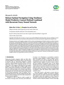
λ (Q ) . Therefore, by LaSalle’s The condition, V& is definite negative, is held when γ < min 2 λ max ( P ) invariance theorem, the origin is asymptotically stable. The global asymptotic stability of the estimated closed loop system with uncertainties is guaranteed. 6 SIMULATION RESULTS We consider the two-link rigid robot manipulator to illustrate the performances of the controller with uncertainties compensation expressed by the observers equations (35) and (36) respectively. The structure of the robot system driven by NMPC is shown in figure 1. The detail about the robot model is given in appendix. The model is simulated with a sample time of 10-4s and the initial values of angular positions velocities are qˆ (0) = 0.1 rad and q&ˆ (0) = 0 rad/s respectively for state observer, and q(0) = 0 rad and q& (0) = 0 rad/s respectively for robot model. The parameters of the controller, uncertainties observers and state observer are chosen by trial and error in order to achieve accurate performances.
Figure 1: Robust estimated nonlinear model predictive control for two-link rigid robot. Int. J. of Appl. Math and Mech. 5(1): 48-59, 2009.
Robust Nonlinear Predictive Control Based on State Estimation for Robot Manipulator
59
First, the tracking performance of robot system, driven by the nonlinear model predictive control law (34), is tested without the uncertainties observer. The robot system is affected by external disturbance b, which has the value 10 in the time interval [0.5s 4s]. The disturbance term is included in the robot model and the information about it is not taken into account when carrying out the control law. The values of prediction times are T1=0s, T2=10-3s. The state observer gain is taken as K= [104 0; 0 108]. Figure 2 shows the result for angular positions and tracking errors. It can be seen that small tracking errors, for both joints, are successfully achieved. However, steady errors occur in the system responses. The present situation can be explained by the fact that the control law has no information about the external disturbances in order to compensate their effects. Figure 3 illustrates the induced control torque applied to robot manipulator. Note that the control torque lie inside the saturation limits. From figure 4, we can observe that the estimation errors are good although the presence of steady errors in the responses. As shown in the equation of state observer (31), the information about uncertainties is needed to get an accurate performance.
Figure 2: Angular positions and tracking errors of distributed system without uncertainties compensator ……. reference, estimate
Figure 3: Induced torque control produced from the nonlinear model predictive controller
Figure 4: Error estimation of the nonlinear state observer (controller without compensation) Then, the uncertainties observers (35) and (36) are applied to the control law (34) respectively. The matrix P has the value [106 0; 0 106] and Γ= In×n for the observer (35), and L=[102 0; 0 102] for the observer (36). Figure 5 illustrates the angular positions and tracking errors of the system with uncertainties compensators. The steady error is vanished completely with the compensator (36), which means that the disturbance is well rejected. However, with the compensator (35), the steady error is only reduced compared with the results in figure (2).The elimination of steady errors by the compensator (36) can Int. J. of Appl. Math and Mech. 5(1): 48-59, 2009.
60
A. Merabet and J. Gu
be explained by the presence of the integral action. It is known in control theory that an integral action achieves zero steady state error for constant reference inputs and disturbances. The same observation can be noticed in the result of state estimation errors shown in figure 6, where the uncertainties, carried out by the compensator (36), are included in state observer.
Figure 5: Angular positions and tracking errors of distributed system with uncertainties compensator ….. reference, estimate with compensator (35) , estimate with compensator (36) ….. tracking error with compensator (35), tracking error with compensator (36)
Figure 6: Error estimation of the nonlinear state observer (controller with compensation)
Int. J. of Appl. Math and Mech. 5(1): 48-59, 2009.
Robust Nonlinear Predictive Control Based on State Estimation for Robot Manipulator
61
In case of mismatched model, an unknown load carried by the robot is regarded as part of the second link, then the parameters m2, lc2, I2 will change, m2+∆m2, lc2+∆lc2, I2+∆I2, respectively. The variations values are ∆m2 = 1.5, ∆lc2 = 0.125, ∆I2 = 1/12. Also, the friction (Coulomb and viscous friction) given by Fr (q& ) = Fc sign (q& ) + Fv q& , with values Fc = Fv = diag (5, 5), are added to the robot model. The same parameters values of the controller, disturbance observer (35) and state observer are used as declared above. However, the gain of compensator (36) is decreased L = [70 0; 0 70]. As seen in figure 7, in case of the compensator (36), the errors occur in transient response, for this raison the gain is decreased, then reach zero. In case of the compensator (35), the errors in transient response are smaller than in the first case, but they do not reach zero like the other observer. The results show that the tracking performance is successfully achieved and the effect of external disturbance is well rejected with the compensator (36). Concerning the unmodeled quantities and parametric uncertainties, the nonlinear model predictive controller, combined with uncertainties observer, deals well with their variations. It can be mentioned also that the state estimation, given by the nonlinear observer, is accurate for the tracking performance. The accuracy of the estimated nonlinear model predictive control combined with the compensator (36) is justified by the presence of the integral action, which eliminates steady state error.
Figure 7: Angular positions and tracking errors of mismatched model with uncertainties compensator ….. reference, estimate with compensator (35) , estimate with compensator (36) ….. tracking error with compensator (35), tracking error with compensator (36)
Int. J. of Appl. Math and Mech. 5(1): 48-59, 2009.
62
A. Merabet and J. Gu
7 CONCLUSIONS A robust nonlinear predictive controller based on state estimation for rigid robot is presented in this work. The predictive control law minimizes the quadratic cost function of tracking errors. The solution for the control is analytically derived, without need of online optimization, which enables fast real-time implementation. Two methods are conducted to deal with system uncertainties. The first is based on the theory of guaranteed stability of uncertain systems. It results to an observer, which takes information from system error. The second observer is derived from the nonlinear model predictive control law. It contains an integral action on system errors. This kind of control strategy is robust with respect to modeling errors, very effective in disturbance rejection, and gives no steady error caused by either parameters uncertainties or external disturbances. The estimated nonlinear model predictive control is carried out with the quantities, angular positions and velocities, issued from a nonlinear state observer. It has been shown that the tracking performance is achieved accurately when the uncertainties are well compensated. The global asymptotic stability of the closed loop system is guaranteed and proved analytically. Results are given to illustrate the link position tracking performance of the proposed robust nonlinear predictive controller based on state estimation. APPENDICES The elements of the two-link robot model are given by
D11 = m1l c21 + m 2 ( l12 + l c22 + 2 l1l c 2 cos q 2 ) + I 1 + I 2 ; D12 = D 21 = m 2 ( l c22 + l1l c 2 cos q 2 ) + I 2 ; D 22 = m 2 l c22 + I 2 C 11 = − ( m 2 l 1 l c 2 sin q 2 ) q& 2 ; C 12 = − ( q& 1 + q& 2 ) m 2 l 1 l c 2 sin q 2 ; C 21 = ( m 2 l 1 l c 2 sin q 2 ) q& 1 ; C 22 = 0
G1 = (m1l c1 + m 2 l 1 ) g cos q1 + m 2 l c 2 g cos(q1 + q 2 ); G 2 = m 2 l c 2 g cos(q1 + q 2 ) For i = 1, 2, qi denotes the joint angle; mi denotes the mass of link i; li denotes the length of link i; lci denotes the distance from the previous joint to the center of mass of link i; and Ii denotes the moment of inertia of link i (Spong et al. 2006). The nominal values of robot parameters are: Link 1: m1 = 10 kg, l1 = 1 m, lc1 = 0.5 m, I1 = 10/12 kg-m2. Link 2: m2 = 5 kg, l2 = 1 m, lc2 = 0.5 m, I2 = 5/12 kg-m2.
Int. J. of Appl. Math and Mech. 5(1): 48-59, 2009.
Robust Nonlinear Predictive Control Based on State Estimation for Robot Manipulator
63
REFERENCES Bordon C and Camacho EF (1998). A generalized predictive controller for a wide class of industrial processes. IEEE Transactions on Control Systems Technology, 6(3), pp. 372-387. Cavallo A, De Maria G, and Nistri P (1999). Robust control design with integral action and limited rate control. IEEE Transactions on Automatic Control, 44(8), pp. 1569-1572. Chen WH, Balance DJ, Gawthrop PJ, Gribble JJ, and O’Reilly J (1999). Nonlinear PID predictive controller. IEE Proceedings Control Theory application, 146(6), pp. 603-611. Chen W-H, Balance DJ, Gawthrop PJ and O’Reilly J (2000). A nonlinear disturbance observer for robotic Manipulators. IEEE Transactions on Industrial Electronics, 47 (4), pp. 932-938. Corriou JP (2004), Process Control. Theory and Applications. Springer, London, UK, 2004. Curk B and K. Jezernik K (2001). Sliding mode control with perturbation estimation: Application on DD robot mechanism. Robotica, 19(10), pp. 641-648. Feng W, O’Reilly J, and Balance DJ (2002). MIMO nonlinear PID predictive controller,” IEE Proceedings Control Theory application 149(3), pp. 203-208, 2002. Feuer A and Goodwin GC (1989). Integral Action in Robust Adaptive Control,” IEEE Transactions on Automatic Control, 34(10), pp. 1082-1085. Hedjar R and Boucher P (2005). Nonlinear receding-horizon control of rigid link robot manipulators. International Journal of Advanced Robotic Systems, 2(1), pp. 015-024. Hedjar R, Toumi R, Boucher P, and Dumur D (2002). Feedback nonlinear predictive control of rigid link robot manipulator. Proceedings of the American Control Conference, Anchorage AK, pp. 3594-3599. Heredia JA and Yu W (2000). A high-gain observer-based PD control for robot manipulator. Proceedings of the American Control Conference, Chicago, Illinois, USA, pp. 2518-2522. Khalil HK (1999). High-gain observers in nonlinear feedback control. New Directions in nonlinear observer design. Lecture Notes in Control and Information Sciences, 24(4), pp. 249-68. Klančar G, and Škrjanc I (2007). Tracking-error model-based predictive control for mobile robots in real time. Robotics and Autonomous Systems, 55, pp. 460-469. Kozłowski K (2004), Robot motion and control. Recent developments. Springer, London, UK. Richalet J (1993). Industrial Applications of Model Based Predictive Control. Automatica, 29(5), pp. 1251-1274. Rodriguez-Angeles A, and Nijmeijer H (2004). Synchronizing Tracking Control for Flexible Joint Robots via Estimated State Feedback. ASME Journal of Dynamic Systems, Measurement and Contro,l 126, pp. 162-172.
Int. J. of Appl. Math and Mech. 5(1): 48-59, 2009.
64
A. Merabet and J. Gu
Spong MW, Hutchinson S, and Vidyasagar M (2006), Robot modeling and control. John Wiley & Sons, USA. Vivas A and Mosquera V (2005). Predictive functional control of a PUMA robot. ICGST, ACSE 05 Conference, Cairo, Egypt, pp. 372-387. Wang W and Gao Z (2003). A comparison study of advanced state observer design techniques. Proceedings of the American Control Conference, Denver, Colorado, USA, pp. 4754-4759.
Int. J. of Appl. Math and Mech. 5(1): 48-59, 2009.