Schunck [3] uses clustering of local gradient-based constraints and surface-based smoothing. Odobez and. Bouthemy [4] use an M-estimator based on an affine.
ROBUST MULTIRESOLUTION COMPUTATION OF OPTICAL FLOW E.P. Ong and M. Spann School of Electronic and Electrical Engineering University of Birmingham Birmingham B15 2TT, U.K. handle cases of the neighbourhood straddling two or three motions.
ABSTRACT This paper presents an algorithm that provides good estimates of the optical flow at motion discontinuities and occlusion regions based on the least-median-squares robust estimator. The use of a multiresolution scheme enables optical flow to be computed for objects with large motions. A movable overlapping neighbourhood strategy eliminates block-effects and also deals with cases of the local neighbourhood straddling regions of two or three motions. Results for both synthetic and real image sequences are presented. A quantitative comparison with the matching technique of Anandan and the differential technique of Odobez and Bouthemy shows that the proposed algorithm gives much lower angular and absolute errors and hence performs much better than the other two methods.
2. DESCRIPTION OF ALGORITHM 2.1. Least-Median-Squares (LMS) Motion Estimator The computation of the optical flow is based on the motion constraint equation [6]: ∇I ( x , t )T u ( x , t ) + It ( x , t ) = 0 (1) is the brightness function, where I ( x, t ) ∇I ( x , t ) = ( Ix ( x , t ), Iy ( x , t ))T , Ix ( x , t ) , Iy ( x , t ) and It ( x , t ) are the partial derivatives of I ( x , t ) with respect to space and time at the point ( x , t ) ; u = ( u, v )T is the flow vector with flow velocities, u and v, in both x and y directions, and x = ( x , y ) . The flow field, u, can be modelled by a 2-D polynomial motion model [4]. An affine motion model is defined as: u ( x ) = Ax T + b (2)
1. INTRODUCTION
a0
Computation of optical flow is an essential step prior to several important image processing operations and many different methods such as differential, correlation, energy, and phased-based techniques [1] have been proposed. Several approaches have been proposed in order to overcome the problems faced in computing optical flow at motion discontinuities and occlusion regions. Heitz and Bouthemy [2] use both gradient-based and featurebased motion constraints based on Markov random fields. Schunck [3] uses clustering of local gradient-based constraints and surface-based smoothing. Odobez and Bouthemy [4] use an M-estimator based on an affine motion model of the gradient-based motion constraint equation. To compute the optical flow for objects with large motions, multiresolution schemes have been used [5][4]. In this paper, an affine model of the flow field based on the motion constraint equation and leastmedian-squares regression has been adopted for the local computation of the optical flow. The use of a multiresolution scheme enables the flow to be computed for objects with large motions. Movable overlapping neighbourhoods are used to eliminate block-effects and to
where A = a2
a1 , b = ( u0 , v0 )T . a 3
The error in
modelling the motion field at a point x is given by: r ( x ) = ∇I ( x , t )T u ( x , t ) + It ( x , t )
(3)
The above equation can be rewritten as: r ( x ) = a ( x )T Θ − y ( x )
(4)
where
a ( x ) = ( Ix , xIx , yIx , Iy , xIy , yIy ) , Θ = ( uo , a0 , a1 , v0 , a2 , a3 )T , y ( x ) = − It ( x ) . T
The motion parameters are computed using LMS regression [7] by solving: $ = arg min med r ( x , Θ ) 2 Θ (5) Θ
x ∈R
where R is the neighbourhood for computing optical flow. The motion parameters are then refined using weighted least-squares to improve the relative efficiency of the LMS algorithm [7].
1
coarsest resolution (level P) of the pyramid and the $ p , b$ p ) computed for all optimum motion parameters ( A blocks. Then, an incremental motion estimate scheme is employed to obtain the incremental motion estimates $ p , ∆b$ p ) and hence the refined motion estimates ( ∆A $ ( A p , b$ p ) at the next finer level (level p). The $ p , ∆b$ p ) (which are the incremental motion estimate ( ∆A estimates for ( ∆A p , ∆b p ) ) is obtained by solving [8]:
2.2. Implementation Strategy The above-mentioned LMS motion estimator is used to compute the optical flow in each local neighbourhood from 2 successive frames of images. The neighbourhoods are derived by dividing the image into overlapping blocks, each block overlapping its immediate neighbours by 50%. The overlapping neighbourhood strategy eliminates block-effects commonly faced by local methods for computing optical flow. Block-effects prevent accurate estimation of the flow around the boundary regions of the moving objects. The motion parameters are also computed for each block shifted from its nominal location by a quarter of the distance between adjacent neighbourhoods in both x and y directions. The final motion parameters for each block are the parameters computed with the maximum number of inliers. This step prevents inaccurate parameter estimates when the block straddles regions containing three motions and none of the motions make up 50% of the points in the block. This effect can be seen in Figure 1 where the original neighbourhood location encounters sucha a situation and the shifted neighbourhood location causes more than 50% of the points in teh neighbourhood to correspond to the motion on the right sphere and hence solves the ambiguous problem. In addition, this step also prevents inaccurate parameter estimates when the block straddles regions containing 2 motions with the same number of supporting points for each motion.
∇I ( x p + 2 δx$ p +1 , t + δt ) • ( ∆A px p + ∆b p ) δt +
I ( x p + 2 δx$ p +1 , t + δt ) − I ( x p , t ) = 0
(6)
$ p +1x p +1 + b$ p +1 ) δt is the current where 2 δx$ p +1 = 2 ( A displacement estimate from the previous level (level p+1), and δt is the time step between two successive frames. The estimated motion parameters at each pyramid level is given by [8]: P −1
$ p = ∑ ∆A $i +A $ P; A i= p
P −1
b$ p = ∑ 2i − p ∆b$ i + 2 P − p b$ P
(7)
i= p
where P is the coarsest resolution level and p is the current resolution level. At the finest resolution, each point in the image may have no associated motion parameters or it may have more than one set of estimated motion parameters. The motion parameters corresponding to the smallest sum of robust scale estimate will then be assigned to each point.
With the overlapping neighbourhood strategy, each point in the image may have no associated motion parameters or it may have more than one set of estimated motion parameters. The motion parameters corresponding to the smallest robust scale estimate will then be assigned to each point.
3. RESULTS 3.1. Synthetic Images Figure 1(a) shows one frame of the synthetic image sequence. Each frame is 256x256 pixels. The left sphere is moving to the left at about 2.5 pixels per frame, while the right sphere is diverging outwards with a maximum speed of about 3.4 pixels per frame. The square block is moving vertically downwards at 6 pixels per frame. Figure 1(b) shows the needle diagram of the true flow field (sub-sampled at an interval of 8 pixels). Figure 1(c) shows the needle diagram of the optical flow computed using the LMS method (using a 3 level quadtree pyramid and 32x32 pixels neighbourhood at the finest resolution). Figure 1(d) shows the needle diagram of the flow computed using Anandan's method [5] (using a 3 level Laplacian pyramid) while figure 1(e) shows that computed using Odobez and Bouthemy's method [4] (using a 3 level Gaussian pyramid and 32x32 pixels neighbourhood at the finest resolution). It can be seen that the LMS method gives the best qualitative results for the computed optical flow field. Block-effects can be seen in the optical flow computed using Odobez and
Figure 1: Effect of shifting the location of the neighbourhood for computing the optical flow 2.3. Multiresolution Scheme The above-mentioned LMS motion estimator is embedded in a multiresolution scheme. This is achieved by first building a quadtree pyramid from the original image. The LMS motion estimator is then applied to the
2
Bouthemy's method while obvious errors have also occurred for Anandan's method.
Odobez & Bouthemy
96.83
5.13
13.16
0.17
0.42
Table 1: Quantitative comparison of different methods for the image sequence shown in Figure 1.
(a)
(b)
3.2. Real Images Figure 2(a) shows one frame of the tree sequence. This image sequence has been obtained by a horizontally translating observer and each frame of the sequence is 180x180 pixels. The horizontal motion on the tree is about 6 pixels per frame. Figure 2(b) shows the needle diagram of the optical flow computed using the LMS method (using a 3 level quadtree pyramid and 32x32 pixels neighbourhood at the finest resolution). Figure 2(c) shows the needle diagram of the flow computed using Anandan's method [5] (using a 3 level Laplacian pyramid) while figure 2(d) shows that computed using Odobez and Bouthemy's method [4] (using a 3 level Gaussian pyramid and 32x32 pixels neighbourhood at the finest resolution). Without a priori knowledge of the actual motion, it is impossible to make a quantitative comparison of the different optical flow methods on this sequence. However, it can be seen that both the LMS and the Anandan's method give reasonable qualitative results, whereas the Odobez and Bouthemy's method is poorer.
(c)
Figure 1: (a) One frame of the spheres sequence. (b) Needle diagram of the true optical flow field. (c) Needle diagram of the optical flow computed using LMS motion estimator. (d) Needle diagram of the optical flow computed using Anandan's method. (e) Needle diagram of the optical flow computed using Odobez and Bouthemy's method. A quantitative comparison of the various methods has also been made using two different error measures: the angular and absolute error. The angular error measure [1] is given by :
r
r
ψ = arccos(v c ⋅ v e )
(
(8)
)
r T r 2 2 where v ≡ 1 / u + v + 1 (u, v,1) , v c is the true r motion vector and v e the estimated motion vector. The absolute error is given by : ψ = vc − ve
Densit y (%)
LMS Anandan
98.31 100
(b)
(c)
(d)
(9)
Table 1 shows the angular and absolute errors given by the various methods for the spheres image sequence shown in Figure 1. The results show that the LMS method gives the lowest absolute and angular errors and hence is better than the other two methods. Method
(a)
Ang. Ave Error 1.20 11.32
Ang. Std Dev. 5.78 16.62
Abs. Ave Error 0.07 0.39
Abs. Std Dev. 0.29 0.77
Figure 2: (a) One frame of the tree sequence. (b) Needle diagram of the optical flow computed using LMS motion estimator. (c) Needle diagram of the optical flow computed using Anandan's method. (d) Needle diagram of the optical flow computed using Odobez and Bouthemy's method. 4. CONCLUSIONS
3
This paper has presented an algorithm that provides good estimates of the optical flow in regions of motion discontinuities, occlusion and also for objects with large motions. The algorithm is based on the application of a least-median-squares robust estimator embedded in a multiresolution scheme to compute the optical flow using the motion constraint equation and a 2-D affine model of the flow. It has been shown that the least-median-squares method gives better results than both Odobez and Bouthemy's and Anandan's methods. The major shortcoming of the least-median-squares algorithm is the high computational cost (The current algorithm takes 1 about 3 2 hour to process a 256x256 pixel image
[8]
sequence on a Sparc-10 workstation whereas the Anandan's method takes about 30 minutes while the Odobez and Bouthemy's method takes about 5 minutes). Note however, that the algorithm is inherently parallel involving identical operations on overlapping blocks. The co-operative stage of the algorithm which chooses the block corresponding to the maximum number of inliers over which to compute the motion estimate can be implemented with a single pass through the image. [1]
[2]
[3]
[4]
[5]
[6] [7]
5. REFERENCES J.L. Barron, D.J. Fleet, and S.S. Beauchemin, "Performance of optical flow techniques", International Journal of Computer Vision, Vol. 12, No. 1, 1994, pp. 43-77. F. Heitz, and P. Bouthemy, "Multimodal estimation of discontinuous optical flow using markov random fields", IEEE Transactions on Pattern Analysis and Machine Intelligence, Vol. 15, No. 12, Dec. 1993, pp. 1217-1232. B.G. Schunck, "Image flow segmentation and estimation by constraint line clustering", IEEE Transactions on Pattern Analysis and Machine Intelligence, Vol. 11, No. 10, Oct. 1989, pp. 1010-1027. J.M. Odobez, and P. Bouthemy, "Robust multiresolution estimation of parametric motion models in complex image sequences", Proceedings of 7th European Conference on Signal Processing, Sep. 1994. P. Anandan, "A computational framework and an algorithm for the measurement of visual motion", International Journal of Computer Vision, Vol. 2, 1989, pp. 282-310. B.K.P. Horn, and B.G. Schunck, "Determining optical flow", Artificial Intelligence, Vol. 17, 1981, pp. 185-203. P.J. Rousseeuw, and A.M. Leroy, Robust regression and outlier detection, John Wiley & Sons, New York, 1987.
4
F.G. Meyer, and P. Bouthemy, "Region-based tracking using affine motion models in long range sequences", CVGIP : Image Understanding, Vol. 60, No. 2, Sep. 1994, pp. 119-140.