Jun 1, 2000 - Borgefors, G., I. Ragnemalm, and G. di: 1991, 'The Euclidean Distance Transform: Finding the Local Maxima and Reconstructingthe Shape'.
Automatic and Robust Computation of 3D Medial Models Incorporating Object Variability Martin Styner, Guido Gerig, Sarang Joshi, Stephen Pizer Dept. of Computer Science, Univ. of North Carolina, Chapel Hill NC 27599, USA Jun 01, 2000 Abstract. This paper presents a novel processing scheme for the automatic and robust computation of a medial shape model which represents an object population with shape variability. The sensitivity of medial descriptions to object variations and small boundary perturbations are fundamental problems of any skeletonization technique. These problems are approached with the computation of a model with common medial branching topology and grid sampling. This model is then used for a medial shape description of individual objects via a constrained model fit. The process starts from parametric 3D boundary representations with existing point-to-point homology between objects. The Voronoi skeleton of each sampled object boundary is partitioned into non-branching medial sheets and simplified by a novel pruning algorithm using a volumetric contribution criterion. Using the surface homology, medial sheets are combined to form a common medial branching topology. Finally, the medial sheets are sampled and represented as meshes of medial primitives. Results on populations of up to 184 biological objects clearly demonstrate that the common medial branching topology can be described by a small number of medial sheets and that even a coarse sampling leads to a close approximation of individual objects. Keywords: Medical Imaging,Shape Analysis,Voronoi Skeleton,Medial Shape Description,Skeleton Pruning
to be published in International Journal on Computer Vision
1. Introduction Representation and analysis of shape is considered a difficult and challenging problem in computer vision and image analysis. This paper specifically addresses shape representation of 3D objects, for example anatomical objects extracted from 3D medical image data or new types of 3D models in computer graphics applications. In contrast to most other research studies on object shape, a major emphasis is put on objects expressing shape variability and on representations appropriate for shape discrimination and statistical shape analysis of group differences. Research on methods for representing shape can be broadly categorized into the following categories where shape is defined by a) c 2002 Kluwer Academic Publishers. Printed in the Netherlands.
ijcv01_shape.tex; 11/03/2002; 14:09; p.1
Automatic and robust 3D medial models
2
corresponding landmarks and space warp with interpolation (Bookstein, 1997), b) a high-dimensional warping between image data and application of the deformation to a segmented object template (Christensen et al., 1994; Davatzikos et al., 1996; Joshi et al., 1997), c) a parameterization of object surfaces (Staib and Duncan, 1996; Brechb¨ uhler, 1995), d) an extraction of characteristic surface features (Subsol et al., 1998; Shen et al., 2001), and e) an extraction of the medial axis and a graph description (N¨af et al., 1996; Siddiqi et al., 1999a; Pizer et al., 1999). This paper focuses on the last and discusses a new approach for 3D medial shape representation, inspired by early research of Blum (Blum, 1967), who claims that medial descriptions are based on a biological growth model and thus a ’natural geometry for biological shape’. The medial axis in 2D captures shape intuitively and can be related to human vision (Burbeck et al., 1996; Siddiqi et al., 1997)). Medial representations are useful in solid modeling for designing and manipulating shapes (Montanvert, 1987), in animation (Herda et al., 2000), in shape recognition (Siddiqi et al., 1999a), in shape analysis (Styner and Gerig, 2001; Yushkevich and Pizer, 2001), in model based segmentation (Joshi et al., 2001; Pizer et al., 1999), in image registration (Pizer et al., 1999), etc. The idea is to represent the object by a fully connected skeletal graph. The terms medial axis and skeleton have been used in the literature almost interchangeably and refer to the same basic shape description concept. The formation of a skeleton can be explained with the well-known prairie fire analogy. Let the object be composed of flammable dry grass, and initiate a fire simultaneously over the whole boundary of the object. The fire propagates towards the center of the object and extinguishes at points, called quench points, where the fire fronts meet. The skeleton of the object is defined as the connected collection of these quench points. If the distance to the original boundary is recorded at every quench point, the object can be fully reconstructed from the skeleton. The advantages of medial descriptions are the object intrinsic coordinate system, the division of shape changes into application-relevant categories of thickening, elongation, and bending, and the characterization of shape changes with locality.In boundary descriptions, the shape analysis of an object undergoing a symmetric growth process yields an outwards deformation at various places. It is very hard to conclude from a boundary shape analysis, how much these deformations correlate, whether they are caused by a single process or multiple processes, and whether they are caused by a growth or deformation process. The shape analysis of a medial description yields for such a case a clear and intuitive answer, the origin and magnitude of the symmetric growth.
ijcv01_shape.tex; 11/03/2002; 14:09; p.2
Automatic and robust 3D medial models
3
The disadvantage of the medial axis transform is its sensitivity to changes of the object boundary. Local boundary noise of small amplitude might produce quite large skeletal changes. Small global noiseless object changes might produce quite large skeletal changes. Therefore, similar objects are unlikely described by an equally similar skeleton. August investigated these skeletal changes (August et al., 1999a; August et al., 1999b). Common practices to deal with the boundary change sensitivity involve smoothing processes of the boundary. August shows that even smoothing itself can introduce new skeletal branches. He also showed that the changes in the branching topology are located in regions of ligature, which is a term introduced by Blum to describe the locations on the skeleton influenced by concave boundary sections. The boundary change sensitivity is a fundamental problem of any skeletonization technique. Medial descriptions have been computed using distance transform methods (Borgefors et al., 1991; Shih and Pu, 1995), or by application of the shrinking/thinning operation (Lam et al., 1992; Tek and Kimia, 1999). The boundary change sensitivity is approached by smoothing the boundary. Kimia (Kimia et al., 1995) and Siddiqi (Siddiqi et al., 1999b) proposed front propagation based skeletonization methods. These methods are very efficient and successful in computing a medial description. They do not result in an explicit description via a linked boundaryskeletal datastructure, but rather in a set of voxel-based primitives. Kimia and Giblin (Giblin and Kimia, 2000) have proposed a medial hypergraph in 3D that completely characterizes the shape of an object. Similar to work in 2D by Siddiqi et al (Siddiqi et al., 1999a) this hypergraph could be used for shape recognition and shape design. The representation of the skeleton via the inner Voronoi diagram from the boundary described by a point set has also been studied intensively in past (Boissonnat and Kofakis, 1985; Brandt and Algazi, 1992). The boundary change sensitivity is approached by a simplification process called pruning that removes irrelevant branches of the Voronoi skeleton. The pruning methods most influential to our work have been developed by Ogniewicz (Ogniewicz and Ilg, 1992) in 2D, N¨af (N¨ af et al., 1996) and Attali (Attali et al., 1997) in 3D. Kimia and Giblin (Giblin and Kimia, 2000) have proposed a medial hypergraph in 3D that completely characterizes the shape of an object. None of the the above methods solve the problem of the boundary change sensitivity in appropriate fashion for applications that need robust medial descriptions like 3D shape analysis. None of the methods described above directly results in a medial description that allows us to identify corresponding medial locations.
ijcv01_shape.tex; 11/03/2002; 14:09; p.3
Automatic and robust 3D medial models
4
The idea of pre-computed sampled medial models for similar objects was proposed by Golland (Golland et al., 1999) and Pizer (Fritsch et al., 1997; Pizer et al., 1999). Imposing a fixed branching topology and a fixed sampling on the medial description deals with the problem of boundary change sensitivity. Also, such models have an implicit correspondence between descriptions of different objects. Golland fits a 2D non-branching medial model into an object’s distance transform in a snake-like fashion. This approach cannot be extended straightforwardly to 3D, neither has it been shown to handle branching skeletons. Pizer takes a multi-scale viewpoint. He proposes the m-rep description, which fits medial models via the implied boundaries to the object boundary at given apertures. Prior to this work, the models have been built manually. Tackling open issues in 3D medial shape representation, we have developed a new processing scheme for the automatic and robust computation of a sampled medial m-rep model that represents not only individual objects but a population of objects. The new modeling scheme includes the partition of the skeleton into non-branching medial sheets and a minimal sampling of each sheet, properties that were lacking so far but are essential for statistical shape analysis (Styner and Gerig, 2001; Gerig et al., 2001). When using a medial model with fixed graph properties, the question arises of how well this model represents the individual objects. We propose that a medial model is an appropriate representation of a class if the model is computed in an automatic and stable way from a training population of the modeled object class. Thus an m-rep model is computed for each object class. This paper is organized as follows. We start with a general description of our proposed scheme to compute the medial model. Then we discuss shape space, common medial branching topology and minimal sampling in detail. Next, the fit process of the medial model to individual objects is described. Next, the stability of the medial model is described. In the results section we present results of our scheme in studies of 3D brain structures.
2. Methods The main problem adressed in this paper is the creation of a stable medial model in the presence of biological shape variability. Given a population of similar objects, how can we automatically compute a stable medial model? The following sections describe the scheme that we developed to construct a medial m-rep model from a population of objects described by boundary parameterization using spherical
ijcv01_shape.tex; 11/03/2002; 14:09; p.4
5
Automatic and robust 3D medial models
Model Topology
1.
2.
SPHARM
Pruned Voronoi
Grid sampling parameters for each medial sheet Common Topology
Common Medial model
3. Figure 1. Computation of a m-rep model from an object population. 1. Shape space definition. 2. Common medial branching computation. 3. Minimal sampling computation.
harmonics (SPHARM). More details of the scheme are described in (Styner, 2001). In overview, our scheme is subdivided into 3 steps and visualized in Fig. 1. We first define a shape space using Principal Component Analysis. From this shape space we compute the common branching topology using pruned Voronoi skeletons that achieves an adequate agreement in volume for a specified fraction of the shape space. Then we calculate the minimal sampling of the m-rep model given a predefined maximal approximation error in the shape space. 2.1. M-rep and SPHARM shape description 2.1.1. M-rep models A m-rep is a linked set of medial primitives (Pizer et al., 1999) called medial atoms, m = (x, r, F , θ). The atoms are formed from two equal length vectors joined at their tails and are composed of 1) a medial position x, 2) a width r, 3) a frame F = (n, b, b⊥ ) implying the tangent
ijcv01_shape.tex; 11/03/2002; 14:09; p.5
Automatic and robust 3D medial models
6
plane to the medial manifold and 4) an object angle θ. The medial atoms are grouped into figures connected via inter-figural links. These figures are defined as unbranching medial sheets and together form the medial branching topology. A figure is formed by a planar graph of medial atoms connected by intra-figural links. The connections of the medial atoms and the figures form a graph with edges representing either inter- or intra-figural links. In the remainder of this text, we will refer to that graph by the term ’medial graph’. Correspondence between objects is implicitly given if the medial graphs are equivalent.
Figure 2. SPHARM and m-rep shape description in an example of a human left hippocampus/amygdala complex. Three figures with differently colored intra-figural links are shown. The medial atoms are red dots and the implied boundary is represented by blue dots.
2.1.2. SPHARM The SPHARM description (Brechb¨ uhler, 1995) is a parametric surface description that can only represent objects of spherical topology. The basis functions of the parameterized surface are spherical harmonics. Kelemen (Kelemen et al., 1999) demonstrated that SPHARM can be used to express shape deformations. SPHARM is a smooth, accurate fine-scale shape representation, given a sufficiently small approximation error. Based on a uniform icosahedron-subdivision of the spherical parameterization, we obtain a Point Distribution Model (PDM) directly from the coefficients via a linear mapping. Point correspondences of SPHARM are determined by normalizing the parameterization to the first order ellipsoid. 2.2. Shape space via PCA As a first step in our scheme, we compute a shape space using Principal Component Analysis (PCA) of parametrized objects. The shape space for a class of objects is derived from a training population. The shape space smoothes the object variability in the training population, thus making the computations of our scheme more stable. We assume that the shape space is an appropriate representation of the object variability. PCA is applied to SPHARM objects ci of the training population
ijcv01_shape.tex; 11/03/2002; 14:09; p.6
Automatic and robust 3D medial models
7
as described by Kelemen (Kelemen et al., 1999). The PCA results in an average object ¯ c and eigenmodes of deformation {(λi , vi )}. The first k eigenmodes {(λ1 , v1 ) . . . (λk , vk )} are chosen to cover at least 95% of the population’s variability. 1 X (ci − ¯ c) · (ci − ¯ c)T n−1 i
(1)
0 = (Σ − λi · In ) · vi ; i = 1 . . . n − 1
(2)
Σ =
k X
0.95 ≤ (
n−1 X
λi )/(
i=0
λj )
(3)
j=0
Spaceshape = {¯ c±2·
p
λi · vi }; i = 1 . . . k.
(4)
A discrete description of the shape space is gained by sampling it either uniformly or probabilistically. These samples form an object set that is a representative sampling of the shape space. All subsequent computations of the model building are then applied to this object set. 2.3. Common medial branching topology This section describes the computation of the common medial branching topology in three steps. First we compute for each object in the shape space its branching topology as a set of medial sheets using Voronoi skeletons. Then we establish a common spatial frame in order to compare the topology of different objects. Finally we determine the common branching topology via a spatial matching criterion in the common frame. Additional details of the methods and implementation can be found in (Styner, 2001). 2.3.1. Medial branching topology of a single object The branching topology of an individual object is represented by a set of medial sheets from the pruned Voronoi skeleton (see Fig. 3). We first calculate a finely sampled PDM from the object described by SPHARM. The inner 3D Voronoi diagram is then calculated from the PDM. The Voronoi diagram is well behaved due to the fact that the PDM is a fine sampling of the smooth SPHARM. Nevertheless, this ’raw’ Voronoi skeleton is very complex and has a large number of branches, so a pruning process is needed to simplify the skeleton. In our scheme, pruning is also used to create a coarse-scale representation of the skeleton. Our novel pruning scheme starts with grouping the Voronoi skeleton into a set of non-branching, non-self-intersecting medial sheets. The grouping algorithm is based on the graph-algorithm originally proposed
ijcv01_shape.tex; 11/03/2002; 14:09; p.7
Automatic and robust 3D medial models
8
Figure 3. The medial branching topology of an object (left) is represented by a set of sheets computed from the pruned Voronoi skeleton (right). The unpruned, ’raw’ Voronoi skeleton is shown in the middle.
by N¨ af (N¨ af et al., 1996). Our extended version uses a cost function based on an orientational continuity criterion. Following the grouping step, an additional merging step has been implemented, which merges similar sheets according to a combined radial and orientational continuity criterion. This means that two neighboring sheets are merged if the merged sheet is still non-branching, and if the orientation and thickness properties of the sheets are similar at the merging edge. Following the merging step, a pruning step is applied. The pruning step first computes significance criteria, as described below, for each medial sheet independently. A simple thresholding at a predefined significance level marks the sheets that are to be pruned. The medial sheets are then pruned using a topology preserving deletion scheme. The pruning of medial sheets usually changes the branching topology of the skeleton by creating new sheets or by merging existing sheets. Therefore, an additional grouping and merging step is performed directly after the pruning step if any sheet was pruned. Then, the skeleton needs to be pruned again with the same criterion. This possibly changes the branching topology again. Thus, the sheet-pruning scheme is applied iteratively and loops through a grouping step, a merging step and a pruning step until no sheet is left to be pruned. Two different global significance criteria are used by the pruning scheme. The criterion that is applied first uses the area-contribution of a sheet si to the manifold, and the second criterion uses the volumetric contribution of the si ’s reconstruction to the object: Carea =
nvertices,si nvertices,skel
(5)
ijcv01_shape.tex; 11/03/2002; 14:09; p.8
Automatic and robust 3D medial models
A
B
C
D
9
Figure 4. Voronoi skeleton pruning scheme applied to a lateral ventricle (side views). A. Original boundary. B: Original Voronoi skeleton (∼ 1600 sheets). C: Reconstructed boundary from pruned skeleton (volum. overlap = 98.3%). D: Pruned skeleton (2 sheets).
Cvolume =
Vskel − Vskel−si Vskel
(6)
The area-contribution criterion does not sufficiently correlate with the contribution of a sheet to the object shape. The volumetric contribution criterion proved to be far superior since it correlates directly with the significance of a sheet to the object shape. However, the volumetric contribution criterion is computationally expensive. Thus as a first step in our pruning scheme the computationally efficient area-contribution criterion is used with a conservative pruning threshold to remove tiny sheets, which are unlikely to have a high significance to the object shape. Then the volumetric contribution criterion is used with a nonconservative threshold to create the final pruned Voronoi skeleton. Fig. 4 shows the result of the pruning scheme applied to a real object. Our experiments show that a considerable reduction of the number of medial sheets is possible with sacrificing only little accuracy of the reconstruction. In fact, using a threshold on Carea of 0.1% and a threshold on Cvolume of 1%, the pruned skeletons of all objects studied so far had a volumetric overlap with the original object of more than 98%.
ijcv01_shape.tex; 11/03/2002; 14:09; p.9
Automatic and robust 3D medial models
10
2.3.2. A common spatial frame for branching topology comparison The problem of comparing branching topologies has already been adressed before in 2D by Siddiqi (Siddiqi et al., 1999a) and others, mainly via matching medial graphs. To our knowledge, there has been no work reported in 3D to date. Siddiqi’s results in 2D and August’s (August et al., 1999a) have shown that the medial branching topology is quite unstable. In 3D, the medial branching topology is even more unstable and ambiguous than in 2D. The best matching algorithms developed for 2D all use optimization methods to solve the NP-hard problem of matching trees in an acceptable time. These algorithms would be computationally less efficient in 3D. Also, they cannot be extended straightforwardly to 3D since the graph of the 3D branching topology of an object of spherical topology is no longer a tree as in 2D but a general graph. Thus, we developed a matching algorithm that is not based on graph matching but on spatial correspondence. The branching topology is thereby not represented as a graph but rather by the spatial distributions of medial sheets. In order to apply such an algorithm, we first have to define a common spatial frame. All objects to be compared are mapped into a common spatial frame by a warped registration (see Fig. 5). In order to minimize the mapping distortions, the average object of the shape space is chosen to provide the common spatial frame. The SPHARM description and its implied PDM are used to create correspondences on the boundary between each object and the template object in the common frame. The correspondence in the whole 3D space is interpolated from the PDM boundary correspondence via thin plate splines (TPS). The TPS-warp thus maps every skeleton into the common frame, where all their PDM boundaries match perfectly. It is note-worthy that the mapped skeleton is no longer the skeleton of the its (mapped) PDM boundary. 2.3.3. Extraction of a common branching topology. Given that all medial sheets of the object set are mapped into a common spatial frame, a matching criterion can be defined to assess how well two different sheets spatially correspond. Visually, a high degree of overlap between matching sheets in the common frame can be observed. The centers of the medial sheets match better than the edges, which are quite sensitive to boundary noise. We developed a robust matching criterion that takes into account the non-isotropic spatial distribution of the Voronoi vertices of the medial sheets. Specifically, for every sheet si the covariance matrix Σi of its Voronoi vertices and the average Voronoi vertices’ locations µi (= sheet center) are computed. This covariance matrix Σi can be seen as an ellipsoid approximating the spatial extension of the medial sheet si . The matching criterion is then computed
ijcv01_shape.tex; 11/03/2002; 14:09; p.10
Automatic and robust 3D medial models
11
Figure 5. Schematic overview of matching procedure
as the paired Mahalanobis distance between the sheet centers: dM aha (si , x) = (x − µi )0 · Σ−1 i · (x − µi ) dM aha (si , µj ) + dM aha (sj , µi ) critM aha (si , sj ) = 2
(7)
critM aha ((µi , Σi ), (µj , Σj )) > threshold = 2 ⇒ no match (8) critM aha ((µi , Σi ), (µj , Σj )) ≤ threshold = 2 ⇒ si and sj match An empirically determined threshold leads to the rejection of a match if the sheet centers are further away than twice the paired Mahalanobis distance. This empirical threshold produced good results with the datasets studied so far, but for objects of different complexity another threshold might be more appropriate. The common branching topology is computed stepwise. First, the topology of the average object is chosen as the initial guess for the common branching topology. Step by step the algorithm chooses a different object of the shape space and compares its branching topology with the current common branching topology until the object set is fully processed. Those sheets that do not correspond to any sheet in the current common branching topology are added to it. This means that every sheet of the whole object set is matched by at least one of the sheets of the final common branching topology. The common
ijcv01_shape.tex; 11/03/2002; 14:09; p.11
Automatic and robust 3D medial models
12
branching topology is a set of medial sheets originating from various objects of the shape space mapped into the common spatial frame. 2.4. Minimal medial sampling An m-rep model is determined by a set of medial sheets and the set of corresponding grid parameters {ni , mi }. In the next section, we describe the algorithm to compute the grid sampling of a single medial sheet given the sheet’s parameters ni , mi . This sampling algorithm is applied to all medial sheets in the common branching topology to compute the m-rep model. Next, we describe how this sampling algorithm is used to compute the minimal medial sampling in the shape space given a predefined maximal approximation error. 2.4.1. Sampling of a single medial sheet The grid sampling algorithm solves following problem: Given a medial sheet from the Voronoi skeleton and a set of m-rep grid dimensions n, m, how can we determine the grid samples for a most uniform grid on the medial sheet? The procedure proposed here computes this sampling on the volumetric reconstruction from the medial manifold rather than on the medial manifold itself since efficient and well-tested algorithms exist for a wide range of image operations on volumetric representations.
A
B
C
D
Figure 6. Computing the sampled medial sheet axis. A: Rendering of sheet. B: Overlay of sheet boundary (purple) with smoothed sheet (blue). C: Overlay of sheet and 1D skeleton of smoothed sheet. D: Overlay of sheet and sampled sheet axis.
The procedure first smoothes the voxel sampling of the medial sheet at its boundary. We compute the 1D skeleton of the smoothed sheet
ijcv01_shape.tex; 11/03/2002; 14:09; p.12
13
Automatic and robust 3D medial models
using an thinning procedure, an extended version of the original parallel thinning algorithm (Fu and Tsao, 1981). After a graph-compilation, the longest path is extracted from the thinning-skeleton to form the medial axis of the sheet. That axis is uniformly sampled. Next, the m-rep grid samples on the grid-edge are computed as the closest sheet boundary points of estimated locations on the directions that are normal to the medial axis in the medial sheet’s tangent plane. Finally, the remaining grid samples are linearly interpolated along the lines connecting medial axis samples and grid-edge samples. These steps of the algorithm are visualized in the Figs. 6 and 7.
Medial sheet axis
Grid−edge estimat ion
Edge projection
I nterpolat e
Sheet/ Edge projection
Figure 7. Visualization of the sampling method. Starting from the sampled axis (top left, boundary in black, eroded boundary in purple, axis in red), the grid-edge (top right, blue) is estimated. The grid-edge is projected to the sheet-boundary (bottom right) and the remaining samples (violet) are interpolated.
Since the computed medial samples do not lie at the locations of the Voronoi vertices, they are bijectively projected to the closest Voronoi vertices of the medial sheet. Since the medial manifold is densely sampled with Voronoi vertices, this projection affects the sample locations only slightly. At the Voronoi vertices, the additional information from
ijcv01_shape.tex; 11/03/2002; 14:09; p.13
14
Automatic and robust 3D medial models
2x6 0.068
3x6 0.045
3x7 0.043
3x12 0.040
4x12 0.033
Figure 8. Sampling approximation errors Epop (bottom row) of the m-rep implied surface (top row, dark blue dots) with the original object boundary (light blue transparent) in a hippocampus structure (ravg = 2.67 mm). The m-rep grid is shown as red lines. The grid sampling parameters are shown in the middle row.
the generating points and the Voronoi neighborhood is used to estimate the m-rep atom properties: position, radius, frame and angulation. The computed m-rep is a good initial estimate to the m-rep description. An additional step is needed in order to get the appropriate m-rep description: the medial atoms are deformed to optimally fit the object boundary. This fitting process is described in the section 2.5. 2.4.2. Minimal sampling in shape space The grid dimensions {ni , mi } are optimized to be minimal while the corresponding m-rep has a predefined maximal approximation error in the shape space. The approximation error is defined as the Mean Absolute Distance (M AD) of the m-rep implied boundary and the original boundary. To make it independent of the object size, the M AD error is normalized by the average radius over all skeletons of the population AD ravg : Epop = Mravg . We use an extended version of a nonlinear-optimization algorithm that uses an (1+1)-Evolutionary Scheme (ES) (Styner and Gerig, 1997) to find the optimal grid sampling dimensions for a set of medial sheets of a single object. The value of the goal-function fopt incorporates the total number of medial samples natoms and the approximation error to the original boundary. If the approximation error is larger than a predefined maximal approximation error Emax , then the goal-function value fopt is penalized: Epop ≤ Emax ⇒ fopt = natoms + Epop otherwise ⇒ fopt = Epop ∗ Cpen
(9)
ijcv01_shape.tex; 11/03/2002; 14:09; p.14
Automatic and robust 3D medial models
15
The penalty constant Cpen was chosen to be 10000, which is an appropriate value for all objects with a minimal grid sampling of less than 100x100. Empirical values for Emax were determined in the range of 5% to 10% of the average radius through tests. In the next step the minimal sampling is computed for the shape space. First, the m-rep model with minimal sampling is computed for the average object as described above. Next, this m-rep model is checked whether it appropriately fits into all objects from the object set. If an object oi of the object set has a larger Epop than Emax , the current m-rep model is not appropriate for the shape space and has to be adjusted. In this case, the algorithm computes a new m-rep model with a minimal sampling for that object oi . This m-rep model becomes the current m-rep model, which has to be checked to appropriately fit the whole object set. After all objects of the shape space have been handled by the algorithm, the resulting m-rep model represents the common m-rep model sought. 2.5. Fit of an m-rep model to an individual object Once a common m-rep model is computed, it is used to describe individual objects via fitting the model into the object boundaries. This fitting process is done in 2 steps. First a good initial estimate is obtained, which is then refined in an optimization step. The initial estimate is computed by a TPS warp of the m-rep model from the common frame into the frame of the individual object using the SPHARM correspondence on the boundary. The warped m-rep model is located quite close to the final position, which allows a robust optimization. Starting from this initial position, a optimization procedure changes the properties of the m-rep model to improve the fit to the boundary (Joshi et al., 2001). The optimization applies to the medial atoms mi,j = {x, r, F , θ} local similarity transformations as well as rotations of the local angulation, Si,j = (α, O, t, β)i,j ∈ [(IR+ × SO(3)) × IR3 ] × [− π2 , π2 ]. The transformed medial atoms are computed as follows, m0i,j = Si,j ◦mi,j = (αi,j Oi,j xi,j +ti,j , αi,j ri,j , Oi,j ◦F i,j , θi,j +βi,j ) (10) As detailed in the remainder of this paragraph, a prior on the local atom transformations Si,j is induced based on the displacement of the implied boundary with an additional neighborhood dependent prior on the translations, guaranteeing the smoothness of the medial manifold. In keeping with the level of locality let B be the portion of the implied boundary affected by the atom mi,j . The prior energy on the local
ijcv01_shape.tex; 11/03/2002; 14:09; p.15
16
Automatic and robust 3D medial models
A
B
C
D
Figure 9. Different stages of the m-rep fit for an individual object oi . Two examples from the object set of a lateral ventricle population. On the left, the object is smaller and on the right it is larger than the common m-rep model. A: Common m-rep model in common frame. B: Common m-rep model in frame oi . C: Warped m-rep model in frame oi . D: Fitted m-rep model in frame oi .
transformation Si,j of the atom mi,j becomes
log P (S) = −
Z
n,m=1
Bi,j
X X ||ti,j − ti+n,j+m ||2 ||y − y 0 ||2 , dy − (σr(y))2 ||xi,j − xi+n,j+m || i,j n,m=−1
where y is the corresponding position on the figural boundary implied by the transformed atom m0 , and ti,j is the translation component of the local transformation Si,j . Association between points on the boundary y and the deformed boundary y 0 is made using the figural coordinate system (u, v, t) described below. The point y 0 is the point on the deformed model having the same coordinates as that of the original point y. The integral in the above prior is implemented as a discrete sum over a set of boundary points by defining a sampling of the (u, v, t) coordinate space and calculating the associated implied boundary before and after an atom deformation.
ijcv01_shape.tex; 11/03/2002; 14:09; p.16
Automatic and robust 3D medial models
17
The continuous medial manifold, defined via a spline interpolation, is parameterized by (u, v), with u and v taking the atom index numbers at the discrete mesh positions. A parameter t ∈ [−1, 1] designates the side of the medial manifold on which an implied boundary point lies. For single figures, boundary correspondences are defined via the common parameterization (u, v, t). Positions in the neighborhood of the implied ˆ where dˆ is the r-proportional signed boundary are indexed by (u, v, t, d), distance to the closest boundary point (u, v, t).
3. Stability Shape space - All model building computations are based on the PCA shape space. In our experiments PCA has shown to be a stable procedure that produces good results in leave-one-out experiments. The PCA shape space stabilizes the computation of the m-rep model by removing shape variations due to noise. Common medial branching topology - Our tests suggest that the stability of the common medial branching topology is good. However, the common branching topology depends strongly on the boundary correspondence. Although we have not experienced problems with the quality of the boundary correspondence, it is evident that for objects with a high degree of rotational symmetry the first order ellipsoid correspondence is not appropriate. In our scheme the SPHARM description could be replaced by boundary descriptions that incorporate local information about appearance and geometry into the correspondence computation, e.g. (Shen et al., 2001). The procedure is quite robust to the ordering of the objects in the shape space. Changing the ordering results in the same graph properties of the branching topology. The originating objects of the medial sheets might change, but the sheets and their spatial distributions remain similar (see also Fig. 10). Minimal sampling computation - The borders of the Voronoi skeleton are sensitive to small perturbations on the boundary, unlike the center part of the skeleton, which is quite stable. Thus the properties of the sampled m-rep atoms are quite stable in the grid center but not as stable at the grid edges. The computation of the grid dimensions for a single population is stable. Our experiments suggest that the grid dimensions for a similar population are likely to be close. M-rep model - If the common medial model for 2 similar populations (e.g., 2 different studies of the same structure regarding the same disease) is computed, we expect the computation of very similar medial branching topologies, similar grid parameters, very similar m-
ijcv01_shape.tex; 11/03/2002; 14:09; p.17
Automatic and robust 3D medial models
{¯ c, c¯, c¯ +
√
√ λ5 , c¯ − 2 λ6 }
18
√ √ {¯ c, c¯, c¯ + 2 λ6 , c¯ − 2 λ6 }
Figure 10. Common branching topology for two different orderings. Top row: color coded sheets with Voronoi vertices. Bottom row: List of shape space locations for objects from which the medial sheets are originating (¯ c = average object). Left: Implemented ordering. Right: Ordering with most differing result. Graph properties are the same and the sheets are similar.
rep properties in the center and less similar m-rep properties at the edge of the grid. The model is constructed for a population only once, and its extraction is mainly deterministic and repeatable. M-rep fit procedure - The m-rep fit procedure uses the boundary correspondence to start from an position that is close to the final position. The change of the m-rep properties during the fit procedure is strongly constrained by a prior on neighboring atoms. This prevents the m-rep atoms from moving freely on the medial sheet if the radial function is constant along a direction. The fit procedure is non-deterministic but the strong prior leads to stability and reliability.
4. Applications on real data The scheme has been applied to different studies with populations of several human brain structures; the overall number of processed cases is shown in parenthesis: hippocampus-amygdala (60 cases), hippocampus (180), thalamus (56), pallide globe (56), putamen (56) and lateral ventricles (40). Fig. 11 presents a selection of the computed models. Three of the studies are presented in more detail in the following paragraphs. 4.1. Hippocampus schizophrenia study The hippocampus structure of an object population with schizophrenic patients (56 cases) and healthy controls (26 cases) was investigated. The goal of the study was to assess shape asymmetry between left side objects and right side objects and also to analyze shape similarity between patients and controls. The model was built on a object population that included the objects of all subjects on both sides, with the
ijcv01_shape.tex; 11/03/2002; 14:09; p.18
Automatic and robust 3D medial models
19
Figure 11. Selection of medial models of anatomical structures in the left and right brain hemisphere (top view). From outside to inside: lateral ventricle, hippocampus, pallide globe.
Figure 12. Six individual m-rep descriptions of the hippocampus study (side view). The visualizations show m-rep grids as red lines, the m-rep implied surface as dark blue dots and the original object boundary in transparent light blue.
right hippocampi mirrored at the interhemispheric plane prior to the model generation. The SPHARM coefficients were normalized for rotation and translation using the first order ellipsoid. The size was normalized with the individual volume. The shape space was defined by the first 13 eigenmodes with every other eigenmode holding less than 1% of the variability in the population. All objects in the shape space had a medial branching topology of a single medial sheet with a volumetric overlap of more than 98%. Thus, the common topology was a single sheet. The computed minimal grid sampling of 3x8 had an Epop error
ijcv01_shape.tex; 11/03/2002; 14:09; p.19
Automatic and robust 3D medial models
20
Figure 13. Four individual m-rep descriptions of the lateral ventricle study (side view). The visualizations show m-rep grids as red lines, the m-rep implied surface as dark blue dots and the original object boundary in transparent light blue.
of less than 5% for all objects in the shape space. The application of this model to the whole hippocampus population of 164 objects generated Epop errors in the range of [0.048 . . . 0.088] with an average error of 0.058. The average radius was 3.0 mm, leading to an average error of 0.17mm. The original sampling was 0.942 x1.5mm, leading to individual m-reps computed with sub-voxel accuracy. Some of the individual m-rep objects are shown in Fig. 12. We applied a shape analysis on these hippocampi using the boundary description and the medial description. We found a significant shape difference between the right hippocampi of schizophrenics and controls (Gerig et al., 2002). The power of the medial shape analysis (p < 0.0001) was considerably improved compared to the boundary shape analysis (p = 0.15). 4.2. Lateral ventricle twin study Another study investigates the lateral ventricle structure in an object population with 10 monozygotic and 10 dizygotic twins. As in the first study, shape asymmetry and similarity analysis were to be determined, so the same processing was performed. The SPHARM coefficients were normalized for rotation and translation using the first order ellipsoid. The size was normalized by the individual volume. The first 8 eigenmodes defined the shape space, which holds 96% of the variability of the population. The medial branching topologies in the object set varied between one to three medial sheets
ijcv01_shape.tex; 11/03/2002; 14:09; p.20
Automatic and robust 3D medial models
21
with an volumetric overlap of more than 98% for each object. The single medial sheet topology of the average object matched all sheets in the common frame since the matching algorithm allows one-to-many matches. Thus, the common medial topology was computed to be a single sheet. The minimal sampling of the medial topology was computed with a maximal Epop ≤ 0.10 in the shape space. The application of this model to the whole population generated Epop errors in the range of [0.057 . . . 0.15] with an average error of 0.094. The average radius was 2.26mm leading to an average error of 0.21mm. Some of the individual m-rep objects are shown in Fig. 13. We applied a medial shape analysis on these lateral ventricles. We found that the shape of lateral ventricles is more similar in monozygotic twins than in dizygotic twins (Styner et al., 2001). 4.3. Hippocampus-amygdala schizophrenia study This study investigated the hippocampus-amygdala compound structure in an object population with schizophrenic patients (15 cases) and healthy controls (15 cases). The purpose of this study was to test the capability of our scheme to deal with multi-sheet branching topologies. We also tested whether the populations of the left and right side objects are similar by computing two models, one for each side’s population, and applying the models to the joined population. The SPHARM coefficients were normalized for rotation and translation using the first order ellipsoid. The size was normalized with the individual volume. The first 6 eigenmodes defined the shape space, which holds more than 97% of the variability of the population. The medial branching topologies in the object set varied between two to five medial sheets with an volumetric overlap of more than 98% for each object. The minimal sampling of the medial topology was computed with a maximal Epop ≤ 0.10 in the shape space. This processing was performed for both side’s population resulting in a left m-rep model and a right m-rep model. The computed m-rep models show that our proposed scheme can handle populations of objects with multi-sheet branching topology. The two m-rep models are not the same but are similar (see Fig. 14). The following properties are different: A) Branching topology: The right model consists of three medial sheets, one sheet less than the left model. The three sheets of the right model each have a matching sheet in the left model, so the right model is a subset of the left model in regard to the branching topology. B) Grid sampling dimensions: The sampling dimensions are similar for all of the sheets that are common to both the left and the right model. C) M-rep atom properties: The m-rep atom properties are similar for the matching
ijcv01_shape.tex; 11/03/2002; 14:09; p.21
22
Automatic and robust 3D medial models
sheets. The properties are more similar for m-rep atoms in the grid center than for those at the grid edge.
left, grid = 9x3, 4x3, 3x2, 3x2
right, grid = 7x3, 4x3, 4x2
Figure 14. Application of the scheme to the populations of the left and right hippocampus-amygdala. The resulting common m-rep models are displayed with the grid sampling dimensions. The models are shown in the frame of each side’s average object.
The approximation errors Epop of the m-rep description for all individuals from the joined left and right population using both m-rep models is shown in table I. The range of the approximation errors for each model and population suggest that the two populations are not the same. The left model is appropriate for the right population, whereas the right model is not appropriate for the left population. Table I. Error ranges for Epop for the models (LM, RM) of the left (LP) and right (RP) hippocampus-amygdala population. The average radius is 3.6 mm. The upper bound of RM/LP is considerably larger than the training error of 0.10.
Epop
LM/LP
LM/RP
RM/LP
RM/RP
0.035 - 0.112
0.038 - 0.100
0.043 - 0.158
0.046 - 0.073
5. Summary and Conclusions This paper presented a new processing scheme for medial shape representation that includes the following novel features. The resulting medial model represents the common branching topology of a range of objects characterized by a predefined shape space. Voronoi skeletons with only a small set of medial sheets were obtained by an improved grouping and pruning method. Point to point correspondence between
ijcv01_shape.tex; 11/03/2002; 14:09; p.22
Automatic and robust 3D medial models
23
medial sheets, a property most essential for building statistical shape models and for shape comparison, was achieved by calculating skeletons from a parametrized surface description with existing correspondence. The dense sampling of the Voronoi skeleton was replaced by a discrete grid with minimal sampling given a predefined degree of approximation. Sensitivity to boundary changes resulting in instability of skeleton edges and branching locations, a fundamental problem of any skeletonization technique, were tackled by starting from smooth parametrized object surfaces and by developing new techniques for combination of the medial sheet topology of similar objects and calculation of a minimal grid sampling. In this work, we described the objects of the training population by SPHARM. The SPHARM description and thus also the derived m-rep is constrained to objects of sphere topology. The stability of the computed m-rep model is good but depends on the quality of the SPHARM boundary correspondence. The SPHARM boundary correspondence has shown to be a good approach in the general case, but it has problems in special cases presenting rotational symmetry. Other choices of boundary descriptions are possible if appropriate correspondence between objects is established on the boundary. The robustness of the m-rep model building depends not only on the boundary correspondence but also on the type of objects studied. The scheme is designed for smooth biological objects. Highly complex objects, like the full brain cortex, or man-made objects with sharp edges and corners are difficult to handle. We did not yet build a medial model for such type of complex objects, but we expect that changes to model building scheme would be necessary. The paired Mahalonobis distance between sheet centers is used as a distance measure for matching medial sheets. There are alternative measures for measuring distance between spatial distributions, e.g. the Bhattacharya Distance or the Kullback-Liebler Distance. We are currently planning to study the influence of other distance measures on the performance of our scheme. The choice of fixed topology and sampling for the medial description has the advantages of enabling an implicit correspondence and stabilizing the medial description. However, a fixed topology m-rep cannot precisely capture an individual object. The determined individual mrep is therefore always an approximation, which is appropriate for a coarse scale m-rep description. The results of processing large series of objects clearly demonstrate the feasibility of a medial representation even with only a few sheets to capture coarse-scale shape of a whole shape population. Shape models calculated by the scheme presented herein are being used for model-
ijcv01_shape.tex; 11/03/2002; 14:09; p.23
Automatic and robust 3D medial models
24
based segmentation and for the detection of group differences between patients and controls. In contrast to surface-based object representation, a medial representation allows analyzing growth and bending independently, a property most desirable for shape description. Symmetric growth only affects the growth property and pure deformation only affects the bending property. In the case of asymmetric growth or deformation with width change, the shape change is reflected by both, growth and local deformation. In shape population studies, a joint statistical analysis of both properties will reflect the different phenomena and will help with a correct interpretation. Also, our shape models provide type, magnitude and locality of shape changes. This makes our medial description the shape representation of our choice for studying biological objects, for example for studying neuro-development and neuro-degeneration in brain research.
Acknowledgements M. Chakos and the MHNCRC image analysis lab at UNC Psychiatry kindly provided the original MR and segmentations of the hippocampi. Ron Kikinis and Martha Shenton, Brigham and Women’s Hospital, Harvard Medical School, Boston provided the original MR and segmentations of the hippocampus-amygdala study. We further acknowledge D. Weinberger, NIMH Neuroscience in Bethesda for providing the twin datasets. We are thankful to Ch. Brechb¨ uhler for providing the software for surface parameterization and SPHARM description. We are further thankful to members of the MIDAG group at UNC for providing the m-rep tools and for comments and discussions about m-rep and other medial descriptions. Following grants partially funded this work: NCI grant CA 47982, UNC Intel grant, MHNCRC grant NIH 156001393A1.
References Attali, D., G. Sanniti di Baja, and E. Thiel: 1997, ‘Skeleton simplification through non significant branch removal’. Image Processing and Communication 3(3-4), 63–72. August, J., K. Siddiqi, and S. W. Zucker: 1999a, ‘Ligature Instabilities in the Perceptual Organization of Shape’. Compter Vision and Image Understanding pp. 231–243. August, J., A. Tannenbaum, and S. Zucker: 1999b, ‘On the Evolution of the Skeleton’. In: Int. Conference on Comp. Vision. pp. 315–322. Blum, T.: 1967, ‘A transformation for extracting new descriptors of shape’. In: Models for the Perception of Speech and Visual Form. MIT Press.
ijcv01_shape.tex; 11/03/2002; 14:09; p.24
Automatic and robust 3D medial models
25
Boissonnat, J. and P. Kofakis: 1985, ‘Use of the delaunay triangulation for the identification and the localization of objects’. In: IEEE Computer Vision and Pattern Recognition. pp. 398–401. Bookstein, F.: 1997, ‘Shape and the Information in Medical Images: A Decade of the Morphometric Synthesis’. Comp. Vision and Image Under. 66(2), 97–118. Borgefors, G., I. Ragnemalm, and G. di: 1991, ‘The Euclidean Distance Transform: Finding the Local Maxima and Reconstructingthe Shape’. In: SCIA Conf. pp. 974–981. Brandt, J. and V. Algazi: 1992, ‘Continous Skeleton Computation by Voronoi Diagram’. Computer Vision, Graphics, Image Processing: Image Understanding 55(3), 329–338. Brechb¨ uhler, C.: 1995, Description and Analysis of 3-D Shapes by Parametrization of Closed Surfaces. Diss., IKT/BIWI, ETH Z¨ urich, ISBN 3-89649-007-9. Burbeck, C., S. Pizer, B. Morse, D. Ariely, G. Zauberman, and J. Rolland: 1996, ‘Linking object boundaries at scale: a common mechanism for size and shape judgements’. Vision Research 36, 361–372. Christensen, G., R. Rabbitt, and M. Miller: 1994, ‘3D brain mapping using a deformable neuroanatomy’. Physics in Medicine and Biology 39, 209–618. Davatzikos, C., M. Vaillant, S. Resnick, J. Prince, S. Letovsky, and R. Bryan: 1996, ‘A Computerized Method for Morphological Analysis of the Corpus Callosum’. Journal of Computer Assisted Tomography 20, 88–97. Fritsch, D., S. Pizer, L. Yu, V. Johnson, and E. Chaney: 1997, ‘Segmentation of Medical Image Objects using Deformable Shape Loci’. In: Information Processing in Medical Imaging. pp. 127–140. Fu, K. and Y. Tsao: 1981, ‘A parallel thinning algorithm for 3-d pictures’. Comp. Graphics and Image Proc. 17, 315–331. Gerig, G., M. Styner, M. Chakos, and J. Lieberman: 2002, ‘Hippocampal shape alterations in schizophrenia: Results of a new methodology’. In: 11th Biennial Workshop on Schizophrenia, Davos. Abstract. Gerig, G., M. Styner, M. Shenton, and J. Lieberman: 2001, ‘Shape versus Size: Improved Understanding of the Morphology of Brain Structures’. In: W. J. Niessen and M. A. Viergever (eds.): Medical Image Computing and ComputerAssisted Intervention, Vol. 2208. pp. 24–32, Springer. Giblin, P. and B. Kimia: 2000, ‘A formal classification of 3D medial axis points and their local geometry’. In: IEEE Computer Vision and Pattern Recognition. pp. 566–573. Golland, P., W. Grimson, and R. Kikinis: 1999, ‘Statistical Shape Analysis Using Fixed Topology skeletons: Corpus Callosum Study’. In: Information Processing in Medical Imaging. pp. 382–388. Herda, L., P. Fua, R. Plankers, R. Boulic, and D. Thalmann: 2000, ‘Skeleton-Based Motion Capture for Robust Reconstruction of Human Motion’. In: Computer Animation, Philadelphia, PA. Joshi, S., M. Miller, and U. Grenander: 1997, ‘On the geometry and shape of brain sub-manifolds’. Pattern Recognition and Artificial Intelligence 11, 1317–1343. Joshi, S., S. Pizer, T. Fletcher, A. Thall, and G. Tracton: 2001, ‘Multi-scale deformable model segmentation based on medial description’. In: Information Processing in Medical Imaging. pp. 64–77. Kelemen, A., G. Sz´ekely, and G. Gerig: 1999, ‘Elastic Model-Based Segmentation of 3D Neuroradiological Data Sets’. IEEE Transactions on Medical Imaging 18, 828–839.
ijcv01_shape.tex; 11/03/2002; 14:09; p.25
Automatic and robust 3D medial models
26
Kimia, B., A. Tannenbaum, and S. Zucker: 1995, ‘Shape, Shocks, and Deformations I: The components of two-dimensional shape and the reaction-diffusion space’. Int. Journal of Computer Vision 15, 189–224. Lam, L., S. Lee, and C. Suen: 1992, ‘Thinning methodologies: A comprehensive survey’. IEEE Trans. Pat. Anal. and Machine Intel. 14, 869–885. Montanvert, A.: 1987, ‘Graph environment from medial axis for shape manipulation’. In: Int. Conf. on Pattern Recognition. pp. 197–203. N¨ af, M., O. K¨ ubler, R. Kikinis, M. Shenton, and G. Sz´ekely: 1996, ‘Characterization and recognition of 2d organ shape in medical image analysis using skeletonization’. In: Mathematical Methods in Biomedical Image Analysis. pp. 139–150. Ogniewicz, R. and M. Ilg: 1992, ‘Voronoi Skeletons: Theory and Applications’. In: IEEE Computer Vision and Pattern Recognition. pp. 63–69. Pizer, S., D. Fritsch, P. Yushkevich, V. Johnson, and E. Chaney: 1999, ‘Segmentation, Registration, and Measurement of Shape Variation via Image Object Shape’. IEEE Transactions on Medical Imaging 18, 851–865. Shen, D., E. Herskovits, and C. Davatzikos: 2001, ‘An adaptive focus statistical shape model for segmentation and shape modeling of 3-D Brain Structures’. IEEE Transactions on Medical Imaging 20(4), 257–270. Shih, F. Y. and C. C. Pu: 1995, ‘A skeletonization algorithm by maxima tracking on Euclidean distance transform’. Pattern Recognition 28, 331–341. Siddiqi, K., A. Ahokoufandeh, S. Dickinson, and S. Zucker: 1999a, ‘Shock Graphs and Shape Matching’. Int. Journal of Computer Vision 1(35), 13–32. Siddiqi, K., S. Bouix, A. Tannenbaum, and S. Zucker: 1999b, ‘The Hamilton-Jacobi Skeleton’. In: Int. Conference on Comp. Vision. pp. 828–834. Siddiqi, K., B. Kimia, S. Zucker, and A. Tannenbaum: 1997, ‘Shape, Shocks and Wiggles’. Image and vision computing 17, 365–373. Staib, L. and J. Duncan: 1996, ‘Model-based Deformable Surface Finding for Medical Images’. IEEE Transactions on Medical Imaging 15(5), 1–12. Styner, M.: 2001, ‘Combined Boundary-Medial Shape Description of Variable Biological Objects’. Ph.D. thesis, UNC Chapel Hill, Computer Science. available at www.ia.unc.edu/public/styner/docs/diss.html. Styner, M. and G. Gerig: 1997, ‘Evaluation of 2D/3D bias correction with 1+1ESoptimization’. Technical Report 179, Image Science Lab, ETH Z¨ urich. Styner, M. and G. Gerig: 2001, ‘Medial models incorporating shape variability’. In: M. F. Insana and R. M. Leahy (eds.): Information Processing in Medical Imaging, Vol. 2082. pp. 502–516, Springer. Styner, M., M. Jomire, D. Jones, D. Weinberger, J. Lieberman, and G. Gerig: 2001, ‘Shape analysis of ventricular structures in mono- and dizygotic twin study’. In: Schizophrenia Research, Vol. 49. p. 167, Elsevier. Abstract. Subsol, G., J. Thirion, and N. Ayache: 1998, ‘A scheme for automatically building three-dimensional morphometric anatomical atlases: application to a skull atla’. Med. Image Analysis 2(1), 37–60. Tek, H. and B. Kimia: 1999, ‘Symmetry Maps of Free-Form Curve Segments Via Wave Propagation’. In: Int. Conference on Comp. Vision. Yushkevich, P. and S. Pizer: 2001, ‘Coarse to fine shape analysis via medial models’. In: Information Processing in Medical Imaging. pp. 402–408.
ijcv01_shape.tex; 11/03/2002; 14:09; p.26