In this paper, we propose to use marginal space learning (MSL) to exploit the recent ad- ... several LV landmarks, such as the LV apex and two annu- lus points.
Robust Object Detection Using Marginal Space Learning and Ranking-Based Multi-Detector Aggregation: Application to Left Ventricle Detection in 2D MRI Images Yefeng Zheng1 , Xiaoguang Lu1 , Bogdan Georgescu1 , Arne Littmann2 , Edgar Mueller2 , and Dorin Comaniciu1 1 Integrated Data Systems Department, Siemens Corporate Research, NJ, USA 2 Magnetic Resonance, Siemens Healthcare Sector, Erlangen, Germany {yefeng.zheng, xiaoguang.lu, bogdan.georgescu, dorin.comaniciu}@siemens.com Abstract Magnetic resonance imaging (MRI) is currently the gold standard for left ventricle (LV) quantification. Detection of the LV in an MRI image is a prerequisite for functional measurement. However, due to the large variations in the orientation, size, shape, and image intensity of the LV, automatic LV detection is challenging. In this paper, we propose to use marginal space learning (MSL) to exploit the recent advances in learning discriminative classifiers [14, 15]. Unlike full space learning (FSL) where a monolithic classifier is trained directly in the five dimensional object pose space (two for position, one for rotation, and two for anisotropic scaling), we train three detectors, namely, the position detector, the position-orientation detector, and the positionorientation-scale detector. As a contribution of this paper, we perform thorough comparison between MSL and FSL. Experiments show MSL significantly outperforms FSL on both the training and test sets. Additionally, we also detect several LV landmarks, such as the LV apex and two annulus points. If we combine the detected candidates from both the whole-object detector and landmark detectors, we can further improve the system robustness even when one detector fails. A novel ranking-based strategy is proposed to combine the detected candidates from all detectors. Experiments show our ranking-based aggregation approach can significantly reduce the detection outliers.
1. Introduction Cardiovascular disease is the number one cause of death in the developed countries, claiming more lives each year than the next seven leading causes of death combined [5]. Early diagnosis of cardiovascular disease can effectively reduce its mortality. Magnetic resonance imaging (MRI)
Figure 1. Detection results for the left ventricle (cyan boxes) and its landmarks (yellow stars for the left ventricle apex and magenta stars for two annulus points on the mitral valve).
accurately depicts cardiac structure, function, perfusion, and myocardial viability with a capacity unmatched by any other single imaging modality. Therefore, MRI is widely accepted as a gold standard for heart chamber quantification [8]. That means the measurement extracted from other modalities, such as echocardiography and computed tomography (CT), must be verified against MRI. Among all four heart chambers, the left ventricle (LV) is of particular interest because it pumps oxygenated blood out to distant tissues
in the entire body. In this paper, we propose a fully automatic and robust method to detect the LV in 2D long-axis view MRI images. Additionally, we also detect several important LV landmarks, such as two annulus points on the mitral valve and the apex. Our approach is generic and can be applied to other object detection problems without or with minor modifications.
1.1. Challenges
Object localization using marginal space learning Input Image
1.2. Overview of Our Approach Discriminative learning based approaches have been proved to be efficient and robust for many 2D object detection problems [2, 4, 7, 11, 13]. In these methods, shape detection or localization is formulated as a classification problem: whether an image block contains the target shape or not. To build a robust system, a classifier only need to tolerate limited variation in object pose. The object is found by scanning the classifier exhaustively over all possible combinations of locations, orientations, and scales. Exhaustive search makes the system robust under local minima. Almost
PositionOrientation-Scale Estimation
Aggregate Multiple Candidates
Detection Result
Figure 2. Object localization using marginal space learning [15]. Object localization using full space learning Input Image
Coarse Estimator
Ccoarse
Automatic LV detection in MRI images is still a challenging problem. First, unlike CT, MRI provides cardiologists the flexibility in selecting the orientation of the imaging plane to capture the best view for diagnosis. On the other hand, this flexibility presents a huge challenge for an automatic detection system since both the position and orientation of the LV are unconstrained in an image. Roughly, the LV is rotation symmetric around its long axis (the axis connecting the LV apex to the center of the mitral valve). The long-axis views are often captured to perform LV measurement. However, the orientation of the LV long axis in the image is unconstrained (as shown in Fig. 1). Previous work [1, 12] on LV detection focused on short-axis views where the LV shape is roughly circular and consistent during the cardiac cycle, thus making the detection problem much easier. Second, a 2D MRI image used in this application only captures a 2D intersection of a 3D object, therefore, a lot of information is lost. Though the LV and the right ventricle (RV) have quite different 3D shapes, in the 2D apical-four-chamber (A4C) view, the LV is likely to be confused with the RV for an untrained eye (see the first three examples in Fig. 1, and Fig. 4 as well). Third, the LV shape changes significantly in a cardiac cycle. The heart is a non-rigid shape, which keeps beating to pump blood to the body. In order to study the dynamics of the heart, a cardiologist needs to capture images from different cardiac phases. The LV shape changes significantly from the end-diastolic (ED) phase (when the LV is the largest) to the end-systolic (ES) phase (when the LV is the smallest). Last but not the least, the images captured by different scanners with different imaging protocols have large variations in intensity (see Fig. 1).
PositionOrientation Estimation
Position Estimation
Bootstrapped Coarse Estimator
C
bootstrap coarse
Fine Estimator 1
Fine Estimator 2
C 1fine
C 2fine
Aggregate Multiple Candidates
Detection Result
Figure 3. Object localization using full space learning with a coarse-to-fine strategy.
all previous work [2, 7, 11, 13] under this framework only estimates the position and isotropic scaling of a 2D object (three parameters in total). However, in order to localize the object more accurately, more pose parameters need to be estimated. In our application, we want to estimate five pose parameters of the LV: two for translation, one for orientation, and two for anisotropic scaling. However, it is a challenge to extend the learning-based approaches to a high dimensional space since the number of hypotheses increases exponentially with respect to the dimensionality of the parameter space. Recently, we proposed a novel technique called marginal space learning (MSL) [14, 15] to apply learning-based techniques for 3D object detection. To efficiently localize the object, parameter estimation was performed in a series of marginal spaces with increasing dimensionality. To be specific, the task was split into three steps: position estimation, position-orientation estimation, and positionorientation-scale estimation (as shown in Fig. 2). After each step, only a few candidates were kept for the following estimation step. For 2D object detection, the degrees of freedom are five and it is possible to apply the learning-based techniques directly in the full parameter space using a coarse-to-fine strategy. We call this approach full space learning (FSL). The diagram of FSL is shown in Fig. 3. First, a very coarse search step is used for each parameter to limit the number of hypotheses to a tractable level. For example, the search step for position can be set to as large as eight pixels to generate around 1000 hypothesis for translation for an image with a typical size of 300 × 200 pixels. The orientation search step is set to 20 degrees to generate 18 hypotheses for the whole orientation range. Similarly, the search step for scales are also set to a large value. Even with this coarse search step, the total number of hypotheses can easily exceed one million (see Section 4). Bootstrapping can be exploited to further improve the robustness of coarse detection. In the fine search step, we search around each candidate using a smaller search step. Normally, we reduce the
search step by half. This refinement procedure can be iterated several times until the search step is small enough. For example, in the diagram shown in Fig. 3, we iterate the fine search step twice. In this paper, we apply MSL to LV detection in 2D MRI images. MSL was originally proposed for 3D object detection [15]. Experiments demonstrated that it could reduce the number of hypotheses by six orders of magnitude, compared to a naive implementation of FSL. Due to the exponential number of hypotheses, FSL simply does not work for a 3D object detection problem, even after using the coarse-to-fine strategy. Therefore, there is no direct comparison experiment between MSL and FSL. For a 2D object detection problem, both methods are applicable. As a contribution of this paper, we perform a thorough comparison experiment on LV detection in MRI images. Experiments show MSL significantly outperforms FSL on both the training and test sets. As shown in Fig. 1, our detection problem is quite challenging due to the large variations. The performance of a single whole-object detector is limited. Challenging detection problems (e.g., pedestrian detection in a crowded environment [7, 13] and nonrigid objection detection [2]) are often attacked with the part-based detection scheme. Besides the LV bounding box, we also train detectors for several LV landmarks, such as the LV apex and two annulus points. If we combine the detected candidates from both the whole-object detector and part detectors, we can further improve the system robustness even when one detector fails. In this paper, we propose a novel ranking-based method to aggregate all available information. A ranking model is trained to sort the LV whole-object candidates according to the amount of support they get from all detectors. Experiments show that using the proposed ranking-based aggregation, we can significantly reduce the detection outliers. In summary, we make two major contributions in this paper. 1. We perform a comparison experiment between MSL and FSL and give an explanation for the superior performance of MSL. 2. We propose a novel ranking-based aggregation scheme for combining the outputs of multiple detectors to improve detection robustness.
2. Part Model for LV In this section, we show our part model for the LV. Besides the LV bounding box (the cyan box in Fig. 4), we also detect the LV apex (point A in Fig. 4) and two annulus points (points C and D in Fig. 4) on the mitral valve. Instead of defining these landmarks as points and training a position detector for each, we define them as boxes. A base box (the magenta box in Fig. 4) is defined as a square that tightly
Figure 4. Part model of the left ventricle (LV) with cyan for the LV bounding box, magenta for the bounding box of two annulus points, and yellow for the LV apex.
bounds two annulus points. The base box is aligned with the axis connecting the annulus points. The apex box is defined as a square centered at the apex and aligned with the LV long axis. We define the LV long axis as the axis connecting the apex and the basal center (point B in Fig. 4), which is the center of two annulus points. There is no standard way to define of the box size for the apex. We set it to half of the distance from the apex to the basal center. Detecting these landmark points as boxes, we can exploit the orientation and implicit size information of the region around the landmarks. The detection results are more robust than using a position detector only. The LV box is defined as a bounding box of the myocardium and aligned with the LV long axis. There are some constraints or geometric relationships encoded in our part model. For example, the LV box and the apex box have the same orientation, while the base box has a similar orientation to the LV box. From the LV bounding box, we can get a rough estimate of the position of the apex and basal center. These geometric relationships are exploited to pick the best detection box for the LV using a ranking-based approach as shown in Section 6.
3. Marginal Space Learning for LV Detection In this section, we present our object detection scheme using marginal space learning (MSL) [15]. To cope with different scanning resolutions, the input images are first normalized to the 1 mm resolution.
3.1. Training of Object Position Estimator To localize a 2D object, we need to estimate five parameters (two for position, one for orientation, and two for anisotropic scaling). As shown in Fig. 2, we first estimate the position of the object in an image. We treat the orientation and scales as the intra-class variations, therefore,
learning is constrained in a marginal space with two dimensions. Haar wavelet features are very fast to compute and have been shown to be effective for many applications [11]. We also use Haar wavelet features for learning in this step. Given a set of position hypotheses, we split them into two groups, positive and negative, based on their distances to the ground truth. A positive sample (X, Y ) should satisfy max{|X − Xt |, |Y − Yt |} ≤ 2 mm,
(1)
and a negative sample should satisfy max{|X − Xt |, |Y − Yt |} > 4 mm.
(2)
Here, (Xt , Yt ) is the ground truth of the object center. Samples within (2, 4] mm to the ground truth are excluded in training to avoid confusing the learning algorithm. All positive samples satisfying Eq. (1) are collected for training. Generally, the total number of negative samples from the whole training set is quite huge. Due to the constraint of computer memory, we can only train on a limited number of negatives. For this purpose, we randomly sample about three million negatives from the whole training set. Given a set of positive and negative training samples, we extract 2D Haar wavelet features for each sample and train a classifier using the probabilistic boosting-tree (PBT) [9]. We use the trained classifier to scan a training image, pixel by pixel, and preserve top N1 candidates (N1 = 1000 throughout the experiments).
3.3. Training of Position-Orientation-Scale Estimator The full-parameter estimation step is analogous to position-orientation estimation except learning is performed in the full five dimensional similarity transformation space. The dimension of each candidate is augmented by scanning the scale subspace uniformly and exhaustively. The ranges of Sx and Sy of the LV bounding box are [56.6, 131.3] mm and [37.0, 110.8] mm, respectively. The search step for scales is set to 6 mm. To cover the whole range, we generate 14 uniformly distributed samples for Sx and 13 for Sy . In total, there are 182 hypotheses for the scale space. A hypothesis (X, Y, θ, Sx , Sy ) is regarded as a positive sample if it satisfies Eqs. (1), (3), and max{|Sx − Sxt |, |Sy − Syt |} ≤ 6 mm,
(5)
and a negative sample satisfies anyone of Eqs. (2), (4), or max{|Sx − Sxt |, |Sy − Syt |} > 12 mm,
(6)
where Sxt and Syt represent the ground truth of the object scales in x and y directions, respectively. Similarly, the steerable features and PBT are used for training.
3.4. Testing Procedure on Unseen Images
3.2. Training of Position-Orientation Estimator Suppose for a given image, we have N1 candidates, (Xi , Yi ), i = 1, . . . , N1 , for the object position. We then estimate both the position and orientation. The parameter space for this stage is three dimensional (2D for position and 1D for orientation), so we need to augment the dimension of candidates. For each candidate of the position, we sample the orientation space uniformly to generate hypotheses for orientation estimation. The orientation search step is set to be five degrees, corresponding to 72 orientation hypotheses. Among all these hypotheses, some are close to the ground truth (positive) and others are far away (negative). The learning goal is to distinguish the positive and negative samples using image features. A hypothesis (X, Y, θ) is regarded as a positive sample if it satisfies both Eq. (1) and |θ − θt | ≤ 5 degrees, (3) and a negative sample satisfies either Eq. (2) or |θ − θt | > 10 degrees,
image rotation [15]. Similarly, the PBT is used for training. The trained classifier is used to prune the hypotheses to preserve only top N2 candidates for object position and orientation (N2 = 100 in our experiments).
This section provides a summary about the testing procedure on an unseen image. The input image is first normalized to the 1 mm resolution. All pixels are tested using the trained position classifier and the top 1000 candidates, (Xi , Yi ), i = 1, . . . , 1000, are kept. Next, each candidate is augmented with 72 hypotheses about orientation, (Xi , Yi , θj ), j = 1, . . . , 72. The trained positionorientation classifier is used to prune these 1000 × 72 = 72, 000 hypotheses and the top 100 candidates are retained, ˆ i , Yˆi , θˆi ), i = 1, . . . , 100. Similarly, we augment each (X candidate with a set of hypotheses about scaling and use the trained position-orientation-scale classifier to rank these hypotheses. For LV bounding box detection, we have 182 scale combinations, resulting in a total of 100 × 182 = 18, 200 hypotheses. For a typical image of 300 × 200 pixels, in total, we test 300 × 200 + 1000 × 72 + 100 × 182 = 150, 200 hypotheses. The final detection result is obtained using clustering analysis (see [11] for details) on the top 100 candidates after the position-orientation-scale estimation.
(4)
where θt represents the ground truth of the LV orientation. Since aligning Haar wavelet features to a specific orientation is not efficient, we use the steerable features to avoid
4. Full Space Learning for LV Detection For comparison, we also implemented a full space learning (FSL) system that directly learns classifiers in the orig-
Table 1. Parameters for full space learning. The “# Hyph” columns show the number of hypotheses for each parameter. The “Step” columns show the search step size for each parameter. The “# Total Hyph” column lists the total number of hypotheses tested by each classifier. The “# Preserve” column lists the number of candidates preserved after each step. X Ccoarse bootstrap Ccoarse Cf1ine Cf2ine
# Hyph 36 1 3 3
Y Step 8 mm 8 mm 4 mm 2 mm
# Hyph 23 1 3 3
θ Step 8 mm 8 mm 4 mm 2 mm
# Hyph 18 1 3 3
Sx Step 20o 20o 10o 5o
inal five-dimensional space. The full space has five parameters (X, Y, θ, Sx , Sy ). Alternatively, we can use the aspect ratio a = Sy /Sx to replace Sy as the last parameter. Due to the high dimension of the search space, a coarse-to-fine strategy is used. The system diagram is shown in Fig. 3. In total we trained four classifiers. At the coarse level, we use large search steps to reduce the total number of testing hypotheses. To be specific, to detect the LV bounding box in a typical image (300 × 200 pixels), we search 36 hypotheses for X, 23 hypotheses for Y , 18 hypotheses for θ, 15 hypotheses for Sx , and 6 hypotheses for the aspect ratio a. The corresponding search steps are shown in the row labeled as “Ccoarse ” in Table 1. In total, we search 36×23× 18×15×6 = 1, 341, 360 hypotheses at the coarse level. Due to the constraint of limited computer memory, we can only randomly sample a small portion of the negative samples for training. We randomly select three million negative samples. Similar to MSL, the Haar wavelet features and probabilistic boosting-tree (PBT) are used to train the coarse classifier Ccoarse . We find that the trained coarse classifier is not robust enough, so we keep as many as 10,000 candidates after the coarse classification step to make sure that most training images have some true positives included in the candidates. After that, we train a bootstrapped classifier (still at the coarse search level). We split these 10,000 top candidates into positive and negative sets based on their distances to bootstrap the ground truth. We train a classifier Ccoarse to discrimbootstrap inate them. Using this bootstrapped classifier Ccoarse , we prune those 10,000 candidates to preserve only 200 top candidates. As shown in Fig. 3, we use two iterations of fine level search to improve the estimation accuracy. In each iteration, the search step for each parameter is reduced by half. Around each candidate, we search three hypotheses for each parameter. In total, we search 35 = 243 hypotheses around each candidate. Therefore, for the first fine classifier Cf1ine , in total we need to test 200 × 243 = 48, 600 hypotheses. We preserve the top 100 candidates after the first fine-search step. After that, we reduce the search step by half again and train another fine classifier Cf2ine . Finally, similar to MSL, clustering analysis is exploited to obtain the final detection result from the top 100 candidates.
# Hyph 15 1 3 3
# Total Hyph
# Preserve
1,341,360 10, 000 × 1 200 × 243 100 × 243
10,000 200 100 100
a Step 16 mm 16 mm 8 mm 4 mm
# Hyph 6 1 3 3
Step 0.2 0.2 0.1 0.05
The number of hypotheses and search step sizes for each classifier are listed in Table 1. In total, we test 1, 341, 360 + 10, 000 + 46, 800 + 23, 400 = 1, 424, 260 hypotheses. For comparison, only 150,200 hypotheses are tested in MSL. The speed of the system is roughly proportional to the number of hypotheses, therefore, using MSL we can gain a speed-up by a factor of nine.
5. Comparison Experiments of MSL and FSL In this section, we quantitatively evaluate the performance of marginal space learning (MSL) and full space learning (FSL) for LV detection in MRI images. We have 795 MRI images of the LV long-axis view. We randomly select 400 images for training and reserve the remaining 395 images for testing. Two error measurements are used for quantitative evaluation, the center-center distance and the vertex-vertex distance. Given a box with four vertices V1 , V2 , V3 , V4 , we can consistently sort these four vertices based on the box orientation. The vertex-vertex distance is defined as the mean Euclidean distance between the corresponding vertices, 4
Dv (A, B) =
1X A kV − ViB k. 4 i=1 i
(7)
The center-center distance only measures the detection accuracy of the box center, while the vertex-vertex distance measures the overall estimation accuracy in all five pose parameters. Table 2 shows detection errors of the LV bounding box obtained by MSL and FSL. It is quite clear that MSL achieves much better results than FSL. The mean centercenter error is 13.49 mm for MSL and 43.88 mm for FSL. MSL achieves 21.39 mm in the mean vertex-vertex error, compared to 63.26 mm for FSL. MSL was originally proposed to accelerate 3D object detection [15], but in this application to 2D object detection, it also improves detection accuracy. The system performance is dominated by the first detector, the position detector in MSL and the coarse detector Ccoarse in FSL. If a true hypothesis is missed by the first detector, it cannot be picked up in the following steps. Studying these two detectors can give us some hints one the
difference in detection accuracy. Since the same feature sets (Haar wavelet features) and learning algorithm (PBT) are used in both detectors, the superior performance of MSL may come from the following two factors: the sampling ratio of the negative training set and the variation of positive samples. Generally, the number of negative samples is overwhelmingly larger than that of positive samples in a learning-based approach. Due to the constraint of computer memory, almost all learning-based systems [4, 11] can only be trained on a limited number of negative samples. In our case, we randomly select three million negatives to train the classifiers in both MSL and FSL. In FSL, the sampling ratio for negative samples is about 0.35% since there are so many hypotheses to test. On the selected training set with three million negatives, the classifier Ccoarse in FSL was well trained, but it did not generalize well on unseen data since it was trained on relatively too few samples. This is an inherit limitation of FSL due to the exponential increase of the hypotheses. In MSL, the search space has only two dimensions for the position detector. With the same number of negative training samples (three million), the sampling ratio is significantly higher, about 17% of the whole negative set. Therefore, the generalization capability of the position detector in MSL is much better. The second reason for the performance difference may come from the variations of positive samples. To make the trained system robust, the positive samples should be accurately aligned [10]. On the other hand, to achieve a reasonable speed, we have to set large search steps for the coarse classifier in FSL. Therefore, the positive samples in FSL have large variations in all five parameters (position, orientation, and scales). For the position detector in MSL, the positive samples also have large variations in orientation and scales (actually larger than FSL). However, they are very accurately aligned in position. With less variations, it is easier to learn the classification boundary. MSL is significantly faster than FSL since much fewer hypotheses need to be tested. As shown in Section 4, the number hypotheses tested by MSL is about 10.5% of FSL and the speed is roughly proportional to the number of testing hypotheses. On a computer with a 3.2 GHz processor and 3 GB memory, the detection speed of MSL is about 1.49 seconds/image, while FSL takes about 13.12 seconds to process one image.
6. Ranking-Based Multi-Detector Aggregation Due to the large variations in our dataset, the holistic approach by treating the whole LV as one object may fail on some cases. Since we also want to detect some important LV landmarks, we train three detectors, one for the LV bounding box, one for the apex, and the other for the base (as shown in Fig. 4). Aggregating the detection results from multiple detectors, we can build a system which is robust
even when one of the above detectors fails. Part-based detection approaches have been proposed previously to detect human under occlusion in surveillance video [7, 13] or generic nonrigid objects [2]. In [13], the hierarchical human body model has a fixed geometry, e.g., the foot box is exactly the lower half of the whole-body box. With this rigid geometric model, we can convert the detected part box to the whole-body box and all following reasoning is performed at the whole-body level. Shet et al. [7] proposed a logic-based approach to detect human, which allows a more flexible part model. However, domain specific knowledge need to be manually coded in the logic rule templates. To the other extremity, a loosely coupled star model was used in [2] to model the nonrigid deformation of an object. The detection always starts from the whole-object detector and a whole-object candidate is confirmed if we can detect a part in the inferred position. Such a manually defined aggregation scheme cannot fully exploit the rich information embedded in the detected candidates. In this paper, we propose a learning-based aggregation scheme. We keep top 100 candidates from each detector. A detector tends to fire up around the true position multiple times, while the fire-ups at wrong positions are sporadic. This property has been exploited in the clustering analysis based aggregation scheme [11]. According to this observation, a correct LV bounding box should have many surrounding LV candidates. Furthermore, around the apex of a correct LV box, there should be many detected apex candidates. This is also true for the base candidates. Based on the geometric relationship of the candidates, we learn a ranking model [3] to select the best LV bounding box among all LV candidates. After getting the LV detection result, we run the apex and base detectors again within a constrained range to refine the detection results of landmarks. After that, it is straightforward to recover the landmarks (the apex and two annulus points) from the detected apex and base boxes.
6.1. Ranking Features All ranking features are based on the geometric relationship between the box under study and the other candidate boxes. Given boxes A (X A , Y A , θA , SxA , SyA ) and B (X B , Y B , θB , SxB , SyB ), we can calculate the following four geometric relationships. 1) The centercenter distance, which is defined as Dc (A, B) = p (X A − X B )2 + (Y B − Y B )2 . 2) The orientation distance, which is defined as Do (A, B) = kθA − θB k. 3) The overlapping ratio, which is defined as the intersection area of A and B divided by their union area, O(A, B) = (A ∩ B)/(A ∪ B). 4) The vertex-vertex distance, Dv (A, B) (see Eq. (7)). Given an LV bounding box A, three groups of features are extracted and used to learn the ranking model. The first group of features are extracted from the other 99 LV candi-
Table 2. Comparison of marginal space learning (MSL) with full space learning (FSL) for LV bounding box detection on both the training (400 images) and test (395 images) sets. The error measures are in millimeters.
Full Space Learning Marginal Space Learning
Training Set Center-Center Distance Vertex-Vertex Distance Standard Standard Mean Median Mean Median Deviation Deviation
Test Set Center-Center Distance Vertex-Vertex Distance Standard Standard Mean Median Mean Median Deviation Deviation
9.73 1.31
43.88 13.49
25.62 0.84
1.79 1.15
17.31 3.09
37.32 1.63
date boxes. First, all the other LV boxes are sorted using the vertex-vertex distance to box A. Therefore, we can assign a consistent ordering to the extracted feature set, across different boxes. Suppose box B is another LV box, we extract five features from it, including its detection score (which is assigned by the PBT classifier [9]) and all the above four geometric features between boxes A and B. In total, we extract 99 × 5 = 495 features in this group. The second group is based on the geometric relationship of box A to all 100 LV apex candidates. From box A, we can predict the position of its apex, CpA . (We assign CpA as the center of the box edge on the apex side.) Given an apex box C, three features are extracted: 1) detection score of box C, 2) distance to the predicted position, and 3) orientation distance, Do (A, C). In total, we extract 100 × 3 = 300 features in this group. To assign a consistent ordering to the extracted feature set, the LV apex candidates are also sorted w.r.t. the distance to the predicted apex position, CpA . Similarly, we extract 300 features based on the geometric relationship of box A and the top 100 candidates of the LV base. Including the detection score of box A itself, we have 1 + 495 + 300 + 300 = 1096 features.
5.07 2.82
45.01 24.61
21.01 5.77
63.26 21.39
52.09 30.99
46.49 10.19
Given: Initial distribution D over X × X . Initialize: D1 = D. For t = 1, 2, . . . , T • Train weak learner using distribution Dt to get weak ranking ht : X → R. • Choose optimal αt ∈ R. • Update: Dt+1 (x0 , x1 ) =
Dt (x0 , x1 ) exp[αt (ht (x0 ) − ht (x1 ))] Zt
where Zt is a normalization factor (chosen so that Dt+1 will be a distribution). Output the final ranking: H(x) =
PT
t=1
αt ht (x).
Figure 5. The RankBoost algorithm [3].
corresponds to each individual feature presented in Section 6.1. The final learned ranking function H is an optimal linear combination of T (T = 25 in our experiments) features, T X H(x) = αt ht (x). (9) t=1
6.2. Ranking-Based Aggregation In this section, we present the RankBoost [3] learning algorithm, which is used to select the best LV box from the candidate list. The goal of RankBoost learning is minimizing the (weighted) number of pairs of boxes that are misordered by the final ranking, relative to the given groundtruth. Suppose the learner is provided with ground-truth about the relative ranking of an individual pair of boxes x0 and x1 . Suppose box x1 should be ranked above box x0 , otherwise a penalty D(x0 , x1 ) is imposed. (Equally weighted penalty D(x0 , x1 ) = 1 is used in our experiments.) The penalty weights D(x0 , x1 ) can be normalized to a probability distribution. The learning goal is searching for the final ranking function H that minimizes the ranking loss X rlossD (H) = D(x0 , x1 )δ[H(x1 ) ≤ H(x0 )]. (8) x0 ,x1
Here, δ[.] is 1 if the predicate holds and 0 otherwise. The RankBoost algorithm (as shown in Fig. 5) exploits the boosting technique [6] to minimize the ranking loss (Eq. (8)). In Fig. 5, ht is a weak ranking function, which
The optimal weight αt for each feature ht can be found numerically using the Newton-Raphson method. Interested readers are referred to [3] for more details about the RankBoost algorithm.
7. Experiments on Ranking-Based Aggregation In this experiment, we evaluate the performance of our ranking-based multi-detector aggregation method. We train three detectors (one for the LV bounding box, apex, and base, respectively) on the randomly selected 400 MRI images and tested on the remaining 395 unseen images. The left half of Table 3 shows the detection errors on unseen data if we run three detectors independently. A four-fold cross-validation is performed to test our ranking-based aggregation scheme. We randomly split 395 unseen images to four roughly equal sets. Three sets are used to train the RankBoost model, and the remaining set is used for testing. Rotating the configuration until each set has been used for testing once. The detection errors for the LV bounding box after multi-detector aggregation are listed on the right half of Table 3. Using our ranking-based aggregation
Table 3. Quantitative evaluation for LV bounding box, apex, and base detection accuracy with/without ranking-based multi-detector aggregation on an unseen dataset with 395 MRI images. The errors are measured in millimeters. For the LV bounding box, we list both the center-center and vertex-vertex errors. For the landmarks (the apex and annulus points), we list the Euclidean distance to the ground truth. Mean LV Bounding Box (Center-Center) LV Bounding Box (Vertex-Vertex) Apex Annulus Points
13.49 21.39 22.81 15.77
Independent Detection Standard Median Worst 10% Deviation 24.61 5.77 74.71 30.99 10.19 106.74 45.16 6.09 148.09 21.30 7.35 72.00
scheme, we significantly reduce the detection error. The mean center-center error is reduced from 13.49 mm to 9.86 mm, a 26.9% reduction. The mean vertex-vertex error is reduced about 18.1% from 21.39 mm to 17.51 mm. Rankingbased aggregation also reduces the standard deviation significantly. The reduction in median errors is more marginal since most improvement comes from the images with large detection errors. That means the ranking-based aggregation scheme can significantly improve the system robustness to detection outliers. Using the detected LV bounding box to constrain the searching range for the apex and base, we also achieve much better results than detecting them independently. The mean error of the apex is reduced by 36.1%, from 22.81 mm to 14.56 mm. We also see considerable improvement for annulus points. A few examples of the detection results are shown in Fig. 1.
8. Conclusion In this paper, we proposed to use marginal space learning (MSL) to detect the left ventricle (LV) in MRI images. We performed a thorough comparison between MSL and full space learning (FSL). Experiments demonstrated that MSL outperformed FSL on both the training and test sets. Due to the large variations in MRI images, we proposed to aggregate multiple detectors to further improve the robustness of the system. A novel ranking-based scheme was proposed to select the best LV candidate using the geometric relationship to the other candidates. Combining both holistic and part detectors, we significantly reduced the LV detection outliers on unseen data. Our approach is generic and can be applied to other object detection problems without or with minor modifications.
References [1] N. Duta, A. K. Jain, and M.-P. Dubuisson-Jolly. Learningbased object detection in cardiac MR images. In ICCV, pages 1210–1216, 1999. [2] P. Felzenszwalb, D. McAllester, and D. Ramanan. A discriminatively trained, multiscale, deformable part model. In CVPR, 2008. [3] Y. Freund, R. Iyer, R. E. Schapire, and Y. Singer. An efficient boosting algorithm for combining preferences. J. Machine Learning Research, 4(6):933–970, 2004.
Mean 9.86 17.51 14.56 12.72
Ranking-Based Aggregation Standard Median Worst 10% Deviation 16.44 5.24 48.66 24.71 9.79 82.58 28.33 5.76 86.18 16.35 7.02 54.62
[4] B. Georgescu, X. S. Zhou, D. Comaniciu, and A. Gupta. Database-guided segmentation of anatomical structures with complex appearance. In CVPR, pages 429–436, 2005. [5] W. Rosamond, K. Flegal, and K. Furie et al. Heart disease and stroke statistics—2008 update: A report from the American Heart Association Statistics Committee and Stroke Statistics Subcommittee. Circulation, 117(4):25–146, 2008. [6] R. E. Schapire and Y. Singer. Improved boosting algorithms using confidence-rated predictions. Machine Learning, 37(3):297–336, 1999. [7] V. D. Shet, J. Neumann, V. Remesh, and L. S. Davis. Bilattice-based logical reasoning for human detection. In CVPR, 2007. [8] L. Sugeng, V. Mor-Avi, and L. Weinert et. al. Quantitative assessment of left ventricular size and function: Side-byside comparison of real-time three-dimensional echocardiography and computed tomography with magnetic resonance reference. Circulation, 114(7):654–661, 2006. [9] Z. Tu. Probabilistic boosting-tree: Learning discriminative methods for classification, recognition, and clustering. In ICCV, pages 1589–1596, 2005. [10] Z. Tu, X. S. Zhou, A. Barbu, L. Bogoni, and D. Comaniciu. Probabilistic 3D polyp detection in CT images: The role of sample alignment. In CVPR, pages 1544–1551, 2006. [11] P. Viola and M. Jones. Rapid object detection using a boosted cascade of simple features. In CVPR, pages 511–518, 2001. [12] J. Weng, A. Singh, and M. Y. Chiu. Learning-based ventricle detection from cardiac MR and CT images. IEEE Trans. Medical Imaging, 16(4):378–391, 1997. [13] B. Wu, R. Nevatia, and Y. Li. Segmentation of multiple, partially occluded objects by grouping, merging, assigning part detection reponses. In CVPR, 2008. [14] Y. Zheng, A. Barbu, B. Georgescu, M. Scheuering, and D. Comaniciu. Fast automatic heart chamber segmentation from 3D CT data using marginal space learning and steerable features. In ICCV, 2007. [15] Y. Zheng, A. Barbu, B. Georgescu, M. Scheuering, and D. Comaniciu. Four-chamber heart modeling and automatic segmentation for 3D cardiac CT volumes using marginal space learning and steerable features. IEEE Trans. Medical Imaging, 27(11):1668–1681, 2008.