At test time, to generate features x, we simply resize the image for ... is the resized image size. We note that ..... network.org/challenges/VOC/voc2006/results.pdf.
Proposal Generation for Object Detection using Cascaded Ranking SVMs Ziming Zhang
Jonathan Warrell Philip H. S. Torr Oxford Brookes University Oxford, UK
http://cms.brookes.ac.uk/research/visiongroup
Abstract
Typically, we do not want to evaluate a complex classifier at all possible positions, scales and aspect ratios in an image, but only a limited number. We specifically address the problem of generating proposals of bounding boxes rather than presenting a full detection system, and our method can be used as an initial step for any more complex classifier. Using the same overlap-recall evaluation for this problem as [13], we achieve state-of-the-art results.
Object recognition has made great strides recently. However, the best methods, such as those based on kernelSVMs are highly computationally intensive. The problem of how to accelerate the evaluation process without decreasing accuracy is thus of current interest. In this paper, we deal with this problem by using the idea of ranking. We propose a cascaded architecture which using the ranking SVM generates an ordered set of proposals for windows containing object instances. The top ranking windows may then be fed to a more complex detector. Our experiments demonstrate that our approach is robust, achieving higher overlap-recall values using fewer output proposals than the state-of-the-art. Our use of simple gradient features and linear convolution indicates that our method is also faster than the state-of-the-art.
Various methods have been proposed to handle this problem. Branch and bound techniques [13, 14] for instance limit the number of windows that must be evaluated by pruning sets of windows at a time whose maximal response can be bounded above. The efficiency of such methods is highly dependent on the strength of the bound, and the ease with which it can be evaluated, which can cause the method to offer limited speed-up for non-linear classifiers. Alternatively, cascade approaches [4, 8, 17] use weaker but faster classifiers in the initial stages to prune out negative examples, and only apply slower non-linear classifiers at the final stages. In [17] a fast linear SVM is used as a first step, while the jumping window approach [4] builds an initial linear classifier by selecting pairs of discriminative visual words from their associated rectangle regions. Felzenszwalb et al. [9] propose a part-based cascade model using a latent SVM in which part filters are only evaluated if a sufficient response is obtained from a global “root” filter, and [8] propose a combination of cascade and branch and bound techniques. Such approaches have been proved to be efficient, and have generated the state-of-the-art results [9]. However, the fact that in [8] the decision scores for detections must be compared across the training data may limit the efficiency of the early cascade stages, where we only need to compare the scores of a classifier at any level of the cascade within a single image. Further, such approaches learn a single model which is applied at varying resolutions. Recent work [16] strongly suggests that we should explicitly learn different detectors for different scales.
1. Introduction In object detection, we are interested in localizing instances of an object within an image, typically providing as output a set of windows containing object instances. Object detection can be treated directly as a regression problem, where the task is to predict the location and scale of a single object from an image (or its absence), or a classification problem, where the task is to classify every window in an image as either containing an object or not. Recent methods have followed both these approaches, e.g. support vector machines (SVMs) [5], ranking SVM [2], latent SVM [9], multiple kernel learning [17] and structural regression [1]. With the help of non-linear kernels, more training data, more features etc., these methods have achieved better and better detection performance on the public datasets (e.g. the detection tasks in the PASCAL VOC challenge), but unfortunately with longer and longer computational time. The need to accelerate the evaluation process without hurting detection accuracy is thus becoming more important for a successful object detection system, and recently this problem has attracted much attention [4, 8, 13, 14, 17].
We outline here a two-stage cascade model, onto which further stages can be added for a complete detection system. Our approach copes with the problems above as fol1497
Figure 1. Summary of our method. An image (a) is first convolved with
Figure 2. Our scale/aspect-ratio quantization scheme can be represented
a set of linear classifiers at varying scales/aspect-ratios (b) producing response images (c). Local maxima are extracted from each response image, and the corresponding windows with top ranking scores are forwarded to the second stage of the cascade. Each proposed window is associated with a feature vector (d), and a second round of ranking orders these proposals (e) so that the true positives (marked as black) are pushed towards the top during training. Our method outputs the top ranking windows in this final ordering.
hierarchically. (a) superimposes the four window scales in a miniquantization scheme with η = 0.5, and (b) unfolds the scales into a tree structure. The relative widths and heights of the windows are represented by the (w, h) pairs. Such a hierarchy can represent all windows to ηaccuracy (see Section 2.1.1). This figure is best viewed in color.
• T : the set of all possible windows (i.e. bounding boxes) in an image; • S(w, h): the set of all the windows in an image with width w and height h; • o(t, s): the overlap between window t ∈ T and window s ∈ S; • η ∈ [0, 1]: overlap threshold for detection (see Sec. 2.1.1); • k: a given scale/aspect-ratio combination in our quantization scheme; • Sk : the set of all the windows which can be represented to η-accuracy at quantized scale/aspect-ratio k (see Sec. 2.1.1); • wk : a classifier learned for quantized scale/aspect-ratio k.
lows. First, we learn a ranking SVM at each stage in our cascade. The ranking SVM is a normal SVM with the additional constraint that some data should be classified with a higher score than others, e.g. those windows that better overlap the object ground-truth bounding boxes. Ranking SVMs have been used recently in object detection [2] and segmentation [3, 11, 15]. In [2] the ranking objective is applied globally so that positive windows are ranked above negatives across the training set, providing a principled way of learning a one-stage detector with unbalanced training data. For proposal generation, we require only that windows are ranked consistently within a single image, and we show that by adding ranking constraints into the training for the early stages in a cascade we can achieve state-of-theart performance in terms of the overlap-recall metric introduced in [13, 17]. Second, our two-stage cascade enables us to incorporate variability in scale and aspect ratio, where the first stage trains a set of classifiers separately for each scale/aspect-ratio, and the second stage trains a classifier for the windows proposed by the first to achieve a final ranking list. Finally, the usage of simple gradient features and linear convolution makes our method achieve the state-of-the-art performance in terms of speed. Fig. 1 summarizes our approach. The rest of the paper is organized as follows. We describe our cascade design in Section 2, where the first stage finds and ranks local maxima independently at each scale/aspect-ratio (Section 2.1), and the second ranks them across all the scales/aspect-ratios (Section 2.2). In Section 3, we compare our performance with that of [13] in terms of detection quality and running time. Finally Section 4 concludes the paper.
In our training data, each image is annotated with the bounding boxes of the objects of interest. Our goal is to give a higher rank to the windows with a larger overlap with a ground-truth bounding box within a single image such that the windows at the top of the ranking list can be taken as our object proposals.
2.1. Stage I: Scale/Aspect-ratio Specific Ranking The first stage of our cascade aims to pass on a number of object proposals based on different sliding windows at each of a set of quantized scales and aspect ratios to the next stage. This is done by learning a classifier for each scale/aspect-ratio separately. 2.1.1
Scale/Aspect-ratio Quantization
2. Cascaded Ranking SVMs
We design our quantization scheme so that in each image any window t ∈ T can be represented by at least one window s ∈ S in our quantization scheme. Precisely, the overlap between t and s is defined as their intersection area divided by their union area, as shown in Eqn. 1, and we say that s is represented to η-accuracy if o(t, s) ≥ η. T t s S o(t, s) = (1) t s
For ease of explanation of our cascade approach, we list the main notation we use below:
Given the smallest values of width and height, w0 and h0 , we include in our scheme all quantization levels of the 1498
form S(w0 /η a , h0 /η b ), where (a, b) ∈ (0...A, 0...B) is naturally limited by the image size. We can show that using this scheme, a window t with wt ∈ [w0 /η a , w0 /η a+1 ] and ht ∈ [h0 /η b , h0 /η b+1 ] can be represented to η-accuracy by at least one window s ∈ S(w0 /η a , h0 /η b ). The quantization levels can be thought of as forming a tree structure, and Fig. 2 gives an intuitive representation of the scheme. In our experiments, we test η ∈ {0.5, 0.67, 0.75}, which lead respectively to the maximum numbers of classifiers learned at the first stage K ∈ {36, 121, 196} by limiting the sizes of windows from 10 to 500 pixels. 2.1.2
2.1.3
To decide which proposals to forward from the first stage to the second of the cascade, we look for the local maxima in the response image of classifier wk , and set a threshold on the maximum number of windows to be passed on. The first stage thus has two controlling parameters. The first, γ ∈ [0, 2] specifies the ratio between the size of the neighborhood over which we search for the local maxima, and the reference window size for each classifier. The second, d1 ∈ {1 · · · 1000} specifies the maximum number of windows, which are the top d1 ranked local maxima, that can be passed on from any scale. We test the effects of varying these parameters in Section 3.1.1.
Individual Classifier Learning
Since in an image I it is usual to find multiple objects with different ground-truth bounding boxes g1···mI , here we define the maximal overlap of a window t ∈ TI as: ot =
max
i∈{1,··· ,mI }
o(t, gi )
2.2. Stage II: Ranking Score Calibration
(2)
Given η and a set of quantized scales/aspect-ratios, for each scale k we wish to learn a linear classifier wk , as suggested in [16], to rank the windows at that quantized scale/aspect-ratio across the image ITsuch that the ranking score for any window si ∈ Sk TI with osi ≥ η is always higher than that of any window sj ∈ TI with osj < η. That is, for wk we require that within the image I all the corresponding positive training windows T Ik+ = {si ∈ Sk TI |osi ≥ η} should be ranked above all the training negatives I − = {sj ∈ TI |osj < η}. This leads us to formulate the problem as a ranking SVM [12], which can be expressed as below: min wk ,�
s.t.
X 1 kwk k22 + C �nij 2 i,j,n
Proposal Selection
(3)
+ ∀n, i ∈ Ikn , j ∈ In− , wk · (xni − xnj ) ≥ 1 − �nij n �ij ≥ 0
Here, xni and xnj are the feature vectors associated with positive window i and negative window j in training image In respectively, � are the slack variables, C is a non-negative constant, and “·” denotes the dot product operator. In our implementation, for learning wk we simply select all the object ground-truth bounding boxes which can be represented to η-accuracy at scale k as the positive windows, and randomly select the patches from the image as the negative windows. xni are gradient based features using 4 different orientation channels. Recall that the purpose of learning the individual classifier is to build the proposal pool for further usage, so the constraints in Eqn. 3 are restricted to one quantized scale in one image. Therefore, the ranking scores from each classifier are incompatible across scales/aspect-ratios, necessitating the second stage in the cascade.
The first stage of the cascade generates a number of proposal windows at each scale k for image I. The second stage then re-ranks these globally, so that the best proposals across scales are forwarded. To achieve this, we introduce a new feature vector for each window, v, which consists of the channel responses of the classifier at the first stage. For instance, in our implementation v is a 4-dimensional feature vector since feature x is generated using 4 orientation channels, each of which gives a response to the corresponding classifier. The reason for splitting x into different channels is that we can make full use of information in different channels to improve the calibration performance. Based on v, we can re-rank each window i by the decision function f (vi ) = zki · vi + eki , where ki denotes the quantized scale/aspect-ratio associated with window i, zki is a set of coefficients for scale ki that we would like to learn, and eki is the corresponding bias term. Similar to Section 2.1.2, we solve this learning problem using a ranking SVM, and formulate it as an `1 -norm multi-class ranking SVM as shown in Eqn. 4 due to its efficiency in computation and tolerance to noisy data [10], which requires us to learn a separate set of coefficients z for each classifier at the first stage: min
X
z,e,�
k
s.t.
kzk k1 + C
X
�nij
(4)
i,j,n
∀n, i ∈ Iˆn+ , j ∈ Iˆn− , zki · vin − zkj · vjn + eki − ekj ≥ ∆(i, j) − �nij �nij ≥ 0
Here, Iˆn+ and Iˆn− denote the positive and negative windows in image In forwarded from the first stage of the cascade across different quantized scales/aspect-ratios. We note that, as in Eqn. 3, we only generate constraints between positive and negative windows within a image: that is, we are only concerned with generating scores that are locally consistent. Unlike Eqn. 3 though, we introduce a loss function 1499
Figure 3. Cascade design evaluation: γ, d1 , d2 . Higher area under curve (AUC) scores are represented by warmer color. The effects of varying γ (neighborhood size) and d1 (number of candidates selected from the first cascade stage) are tested under various recall regimes by varying d2 (number of candidates selected from the second cascade stage). See Section 3.1.1 for commentary. This figure is best viewed in color.
Figure 4. Quantization and feature evaluation: η, W, H, R. The dimensions of the features are represented as W × R (the classifier width × the number of orientations, and we assume the classifier height H = W ). Performance is measured in terms of average area under recall-overlap curve (i.e. mean AUC), and given under 4 recall regimes, d2 ∈ {1, 10, 100, 1000}. From left to right, the maximum number of classifiers at the first stage K is increased. In general we outperform [13] significantly (also plotted). This figure is best viewed in color.
∆(i, j) which we define in terms of the maximum overlaps of windows i and j: ∆(i, j) = oi − oj , i ∈ Iˆn+ , j ∈ Iˆn−
at the first stage, producing an R-dimensional vector where vr = wk,r · xr . Besides the gradient based features and ranking SVM, we tried simple pixel intensity based features and a normal SVM as well. Due to the page limit, we did not show the comparison in the paper, but the major improvement comes from the ranking SVM rather than the features. At test time, to generate features x, we simply resize the image for each scale k by the ratio of its reference window to (W, H), and then apply the learned classifier wk by 2D convolution. The remaining global parameters of the cascade are γ, d1 and d2 , which affect the trade-off between the number of positive windows we retain at each stage, and the amount of noise we allow through. We investigate the effects of these parameters in Section 3.1.1
(5)
This forces the ranking scores to more closely mirror the ordering of the overlap scores with respect to the object ground-truth bounding boxes in images. In this way, all the windows can be ranked in an image. The top d2 windows are then considered as the final proposals generated at the second stage of our cascade.
2.3. Implementation Details We use simple zero-mean gradient features to learn each classifier wk at the first stage. In detail, we first convert all the images into gray scale, and represent all the object ground-truth bounding boxes to η-accuracy using our scale/aspect-ratio quantization scheme to provide positive windows. After randomly selecting negatives across scales, all windows are resized to a fixed feature window size (W, H), and then for each pixel, the magnitude and orientation of its gradient is calculated. Orientation weights are then calculated in a fixed set of R orientation channels for assigning the gradients to build sub-features xr (r ∈ {1, · · · , R}) separately. Finally, by concatenating all xr , a (W ×H ×R)-dimensional vector is generated consisting of spatial and gradient information. To handle the different illumination contrasts in images, we subtract the mean value to produce a feature vector xi for window i, and the learned classifiers are thus guaranteed to be zero-mean vectors (avoiding the need for a bias in Eqn. 3). The features used at the second stage, v, are produced by concatenating the classifier responses from each orientation channel
2.4. Computational Complexity Our method involves the application of simple linear classifiers to the images, and as such is dominated by the complexity of 2D convolution which must be applied to each image. The complexity can thus be approximated as O(K × R × (W × H) × (WI × HI )), where (WI , HI ) is the resized image size. We note that our complexity is therefore (largely) independent of the number of potential proposals let through at each stage (d1 , d2 ), unlike methods which include non-linear classifiers [13, 17].
3. Experiments We design a comprehensive set of experiments to assess the impact of various parameters and design choices in our model. We also compare our performance against a 1500
Figure 5. Recall-overlap evaluation for VOC2006. Recall-overlap curves are plotted for individual classes using d2 ∈ {1, 10, 100, 1000} from left to right, and K ∈ {36, 121, 196} from top to bottom. All curves are plotted using (W, H, R) = (16, 16, 4). The numbers shown in the legends are the recall percentages when the overlap threshold η is set to 0.5. This figure is best viewed in color.
(a)
(b)
(c)
Figure 6. Recall-proposal evaluation. (a) VOC2006 validation set, (b) VOC2006 test set, (c) VOC2010 validation set. Recall is measured against increasing numbers of output proposals, d2 . Other parameters are fixed at (W, H, R) = (16, 16, 4) and K = 36. Notice that the curves are similar for different classes in all cases, implying we can generalize thresholds from one case to another. This figure is best viewed in color.
3.1. VOC2006
state-of-the-art method [13] and show substantial improvement. We measure our performance in terms of recalloverlap curves [13, 17], which provides a means of assessing the potential information preserved for further processing, and the speed of our method. We test on PASCAL VOC2006 [7] and VOC2010 [6] datasets. VOC2006 consists of 10 object categories, 5304 images of natural scenes, with object labels and their corresponding groundtruth bounding boxes released for training, validation and test sets. VOC2010 consists of 20 object categories, 21738 natural images, and object labels and their corresponding ground-truth bounding boxes are available for training and validation sets only. For training and testing, we split VOC2006 into train/validation and (train+validation)/test, and VOC2010 into train/validation, respectively.
3.1.1
Cascade Design: γ, d1 , d2
We first evaluate the effects of the following cascade parameters: the neighborhood size for finding local maxima γ in the first stage, and the number of windows to be passed on at the first and second stages, d1 and d2 . Fig. 3 shows the performance of various parameter settings in terms of the area under curve (AUC) (i.e. recall-overlap curve) for the class bicycle in VOC2006. We can see that as we move from left to right (increasing d2 ) the area with highest AUC scores shifts from bottom right to top left. This implies more candidates selected from the first cascade stage (high d1 ) and a higher γ are appropriate for low-recall regimes (low d2 ), while the opposite is true for high-recall (high d2 ). For fur1501
Figure 7. Comparing the speed of our method in seconds at various parameter settings. This table is best viewed in color.
Figure 8. Comparing the performance of our method in terms of AUC (%) with that of [13]. We show our performance at two settings, the first (W, H, R, K) = (2, 2, 1, 36) is our fastest setting, with lowest dimensionality. The second (W, H, R, K) = (8, 8, 4, 121) has a similar run time to [13]. Both settings improve on [13] substantially. This table is best viewed in color.
η ∈ {0.5, 0.67, 0.75} respectively. This affects the performance observed, and on the K = 36 graph for instance, we see that the curves are high for η ≤ 0.5, but then drop quickly. Similar drops can be observed in the K = 121 and K = 196 graphs for the corresponding later points in the curves, η = 0.67 and 0.75, implying our quantization is capturing the desired information. The average recalls when d2 = 1000 and η = 0.5 are 95.8%, 97.1%, 96.0% for K ∈ {36, 121, 196} respectively.
ther experiments we choose values d1 = 50 and γ = 0.6, which work well across the d2 settings. 3.1.2
Quantization and Features: K, W, H, R
We next assess the effects on the performance of the features we use (i.e. the size of the classifiers (W, H) and the number of orientations R), and the maximum number of classifiers learned at the first stage K (determined by the overlap threshold η as in Section 2.1.1). Fig. 4 summarizes the results, considering 4 different recall regimes by varying the number of output proposals d2 ∈ {1, 10, 100, 1000}, and comparing them against the best results of [13] in these regimes. Performance is again measured in terms of AUC (averaged across classes). We can see that, as expected, performance increases both as the size of the classifiers and number of orientations increase (W , H, R), and as K increases. However, both of these factors imply longer computational time as discussed in Section 2.4. We see though that even with the smallest feature size, 2×2 with 1 orientation (i.e. only 4-dimensional features), we improve substantially on [13] in most cases and achieve comparable performance otherwise. We will offer further comparison which takes computational time into account. 3.1.3
3.1.4
Recall-Proposal Evaluation
In Fig. 6(a)-(b) we show how the recall is effected as we increase the number of output proposals d2 from 1 to 1000 on the validation and test sets of VOC2006. We fix (W, H, R) = (16, 16, 4) and K = 36. We can see that on both validation and test datasets when d2 is beyond 400, the curves hardly change, which means the AUC for d2 = 400 and d2 = 1000 will be very similar. We believe that this property of our approach is useful for detection tasks, because it narrows down significantly the total number of windows that classifiers need to check while losing few correct detections. In fact, some categories need far fewer proposals to achieve good performance. For instance, for the cat category, 100 output proposals saturates performance. Since the behaviors of our approach on both validation and test sets are quite similar, in practice we can utilize the former to choose a sufficiently small number of output proposals for good performance.
Recall-Overlap Evaluation
Fig. 5 breaks the VOC2006 results down by class, and displays the recall-overlap curves that were used to calculate Fig. 4 for the case of (W, H, R) = (16, 16, 4). We can see here the movement of the curves towards the top-right both as we allow more output proposals (d2 ∈ {1, 10, 100, 1000}) and as we increase K = {36, 121, 196}. Another aspect can be observed from these curves. We recall that our quantized scales/aspect-ratios are designed to cover bounding boxes to a particular overlap threshold of η, so K ∈ {36, 121, 196} corresponds to
3.1.5
Computational Time
Details of our computational time are shown in Fig. 7. Our implementation is a mixture of Matlab and C++, and is run on a single core with 3.33 GHz. The computational time shown here includes all the steps at the test stage, 1502
Figure 9. Comparing the performance of our method in terms of AUC (%) when no scale/aspect-ratio information is included during learning the classifiers (i.e. single classifier), when only aspect ratio information is included, and when both scale and aspect ratio are included. This table is best viewed in color.
Figure 10. Recall-overlap evaluation for VOC2010. Recall-overlap curves are plotted for individual classes using d2 ∈ {1, 10, 100, 1000} from left to right, and K ∈ {36, 121, 196} from top to bottom. All curves are plotted using (W, H, R) = (16, 16, 4). The numbers shown in the legends are the recall percentages when the overlap threshold η is set to 0.5. This figure is best viewed in color.
i.e. calculating features, 2D convolution, proposal selection, and ranking score calibration. As we see, with increase in the size of the feature windows (W, H), the number of orientation channels R, and the maximum number of classifiers learned at the first stage K, computational time grows roughly linearly in the log-scale. This demon-
strates that the computational complexity of our approach can be approximated by the complexity of 2D convolution. Moreover, we can compare our time with the 0.47 ± 0.01 in [13]1 (based on a 2.8 GHz PC). As mentioned, we already 1 In [13], the computational time is only for training models without considering the time for feature extraction.
1503
substantially outperform this method at our fastest setting, (W, H, R) = (2, 2, 1) and K = 36. In Fig. 7 we highlight the closest settings of our method to the speed of [13]. We can see on Fig. 4 that these all offer further substantial improvements, and we make a closer comparison in Fig. 8 by comparing AUC values of [13] with our results at (a) our fastest setting, and (b) the best of our settings with similar computational time. Averaging across the four output settings (d2 ∈ {1, 10, 100, 1000}), [13] achieves 39.9%, while we achieve 44.5% at (W, H, R, K) = (2, 2, 1, 36), and 50.8% at (W, H, R, K) = (8, 8, 4, 121). Our approach is thus quicker, and offers a substantial improvement in output quality to [13].
where different types of features could easily be incorporated at this stage. Our method is both fast and efficient, and we have shown a substantial improvement in speed and recall over a state-of-the-art method [13], which also uses a cascade design. Remaining problems for investigation include how to embed our ranking formulation into a global cost function for a complete detection cascade.
3.1.6
References
Acknowledgements. We thank P. Sturgess, S. Sengupta and L. Ladicky for useful discussion in this paper. This work was supported by the IST Programme of the European Community, under the PASCAL2 Network of Excellence, IST-2007-216886. P. H. S. Torr is in receipt of Royal Society Wolfson Research Merit Award.
Contribution of Scale and Aspect Ratio
[1] M. Blaschko and C. Lampert. Learning to localize objects with structured output regression. In ECCV’08, pages I: 2–15, 2008. [2] M. B. Blaschko, A. Vedaldi, and A. Zisserman. Simultaneous object detection and ranking with weak supervision. In NIPS’10, 2010. [3] S. Bucak, P. Mallapragada, R. Jin, and A. Jain. Efficient multi-label ranking for multi-class learning: Application to object recognition. In ICCV’09, pages 2098–2105, 2009. [4] O. Chum and A. Zisserman. An exemplar model for learning object classes. In CVPR’07, pages 1–8, 2007. [5] N. Dalal and B. Triggs. Histograms of oriented gradients for human detection. In CVPR’05, pages I: 886–893, 2005. [6] M. Everingham, L. Van Gool, C. K. I. Williams, J. Winn, and A. Zisserman. The PASCAL Visual Object Classes Challenge 2010 (VOC2010) Results. http://www.pascalnetwork.org/challenges/VOC/voc2010/workshop/index.html. [7] M. Everingham, A. Zisserman, C. K. I. Williams, and L. Van Gool. The PASCAL Visual Object Classes Challenge 2006 (VOC2006) Results. http://www.pascalnetwork.org/challenges/VOC/voc2006/results.pdf. [8] P. Felzenszwalb, R. Girshick, and D. McAllester. Cascade object detection with deformable part models. In CVPR’10, pages 2241– 2248, 2010. [9] P. Felzenszwalb, R. Girshick, D. McAllester, and D. Ramanan. Object detection with discriminatively trained part-based models. PAMI, 32(9):1627–1645, September 2010. [10] P. Gehler and S. Nowozin. On feature combination for multiclass object classification. In ICCV’09, pages 221–228, 2009. [11] J. Gonfaus, X. Boix, J. van de Weijer, A. Bagdanov, J. Serrat, and J. Gonzalez. Harmony potentials for joint classification and segmentation. In CVPR’10, pages 3280–3287, 2010. [12] R. Herbrich, T. Graepel, and K. Obermayer. Large margin rank boundaries for ordinal regression. In Advances in Large Margin Classifiers, pages 115–132, 2000. [13] C. Lampert. An efficient divide-and-conquer cascade for nonlinear object detection. In CVPR’10, pages 1022–1029, 2010. [14] C. Lampert, M. Blaschko, and T. Hofmann. Efficient subwindow search: A branch and bound framework for object localization. PAMI, 31(12):2129–2142, December 2009. [15] F. Li, J. Carreira, and C. Sminchisescu. Object recognition as ranking holistic figure-ground hypotheses. In CVPR’10, pages 1712–1719, 2010. [16] D. Park, D. Ramanan, and C. Fowlkes. Multiresolution models for object detection. In ECCV’10, pages 241–254, 2010. [17] A. Vedaldi, V. Gulshan, M. Varma, and A. Zisserman. Multiple kernels for object detection. In ICCV’09, 2009.
To verify that our two-stage ranking cascade, involving separate ranking of scales and aspect ratios followed by a calibration, is contributing to our performance, we give further results in Fig. 9 where during learning the individual classifiers we compare our full system against restricted cases where we (a) use only one quantization level, and so do not use scale and aspect ratio information (thus learning only one classifier), and (b) use only aspect ratio information (learning one classifier per aspect ratio). In each case, the feature size is set to (W, H, R) = (16, 16, 4) and K = 36. As shown, we have an average gain in performance as scale and aspect ratio information is added (although in certain classes the effect is less pronounced, and aspect ratio plays a more important role than scale in some).
3.2. VOC2010 We repeat our recall-overlap and recall-proposal evaluations on VOC2010. In Fig. 6(c) we see a similar pattern across classes to the VOC2006 validation and test sets, implying that thresholds can be generalized (even for individual classes) across these datasets. In Fig. 10 we see a similar pattern of results to Fig. 5 (also using the setting (W, H, R) = (16, 16, 4)). The average recalls when d2 = 1000 and η = 0.5 are 86.2%, 92.7%, 91.0% for K ∈ {36, 121, 196} respectively, which are comparable to those in Section 3.1.3. We therefore believe that our approach is robust and efficient across datasets.
4. Conclusion We have introduced a two-stage cascaded model using a ranking SVM framework to generate object detection proposals, which we envisage can be used as the initial stages of a complete object detection pipeline. Our framework naturally incorporates scale and aspect ratio information about objects, which are treated separately in the first stage of the cascade, and we emphasize the flexibility of the framework, 1504