Robust Parametric Modeling Approach Based on Domain Knowledge

Robust Parametric Modeling Approach Based on Domain Knowledge for Computer Aided Detection of Vertebrae Column Metastases in MRI A.K. Jerebko1, G. P. Schmidt2, X. Zhou1, J. Bi1, V. Anand1, J. Liu1, S.Schoenberg2, I. Schmuecking1, B. Kiefer3, and A. Krishnan1 2

1 Siemens Medical Solutions, Inc., Malvern, PA, United States, Department of Clinical Radiology, University of Munich, Munich, Germany, 3 Siemens AG Medical Solutions, Erlangen, Germany

Abstract. This study evaluates a robust parametric modeling approach for

computer-aided detection (CAD) of vertebrae column metastases in whole-body MRI. Our method involves constructing a model based on geometric primitives from purely anatomical knowledge of organ shapes and rough variability limits. The basic intensity range of primary 'simple' objects in our models is derived from expert knowledge of image formation and appearance for certain tissue types. We formulated the classification problem as a multiple instance learning problem for which a novel algorithm is designed based on Fisher’s linear discriminant analysis. Evaluation of metastases detection algorithm is done on a separate test set as well as on the training set via leave-one-patient-out approach. Keywords: vertebrae metastases, computer aided diagnosis.

1 Introduction Whole-body MRI has high sensitivity and specificity for detection of bone-marrow metastases [1],[2]. Spine metastases detection is one of the most important and timeconsuming tasks. In recent years, computer aided detection (CAD) has proven to be efficient help for radiologists if used as a second reader in various applications of computed tomography (CT) and X-rays, such as colonic polyp, lung nodule, breast mass calcification detection, etc. Although lately MRI is becoming a popular screening modality, development of MRI CAD applications is more complicated than that of CT because of intensity in-homogeneity problem and higher noise level. This study evaluates a robust parametric modeling approach based on image formation and anatomical knowledge for computer-aided detection (CAD) of vertebrae column metastases in whole-body MRI. Radiologists usually use T2 STIR pulse sequence for primary vertebrae metastases detection [1],[2]. Although a standard non-contrast protocol of the bone marrow usually implies T1-weighted SE-sequences to discriminate between benign (hemangiomas, osteochondrosis, etc.) and malignant lesions, it is not always acquired N. Karssemeijer and B. Lelieveldt (Eds.): IPMI 2007, LNCS 4584, pp. 713 – 724, 2007. © Springer-Verlag Berlin Heidelberg 2007

in all hospitals. Therefore our CAD scheme was developed for T2 STIR as primary pulse sequence, while resulting CAD marks are shown on T2 STIR and, if available, on T1 images for radiologist review and final diagnosis. Our goal was to develop an algorithm suited to work with alterations in scanning protocols and pulse sequences, such as changes in the level of fat suppression, image resolution, acquisition plane (sagittal or coronal) and tolerant to severe pathological changes in organ appearance. The few methods for vertebrae column segmentation in MR images available in recent literature, such as normalized cuts approach in [3], are not suitable in the case of severe metastases where dissimilarity between healthy and affected vertebrae could be much greater than between vertebrae and other tissue. Our approach involves constructing a model based on geometric primitives from purely anatomical knowledge of organ shape and rough variability limits. The basic intensity range of primary 'simple' objects is derived from expert knowledge of image formation for certain tissue types. Our assumptions include the following: 1) spinal cord, tumors and blood vessels are among the brightest structures in the image for number of MRI pulse sequences (par ex. T2, T2 STIR, HASTE) and, 2) bones are surrounded by cortical bone that does not generate signal in MR images, and therefore it is appears black (it looks like black contour around each bone). The spinal cord detection algorithm presented in section 2 relies only on these basic assumptions. The vertebrae segmentation algorithm described in section 3 also takes into account natural periodicity within vertebral column and requires minimal amount of training data to construct vertebrae column active shape model. The candidate lesion detection and feature extraction scheme are fairly simple and therefore only briefly outlined in section 4, while the main focus is made on a novel classification scheme. The reason for development of specialized classification algorithm is the following: bone metastases detection problem is characterized by multiple manifestation of multifocal or diffuse metastatic disease, while only one CAD detection per vertebrae column segment (cervical, thoracic and lumbar) is enough to bring the structure with multifocal or diffuse pathology into radiologist attention. In case of the focal metastatic disease, each focal lesion should be indicated to the radiologist by a separate mark. We designed a novel classification algorithm for detecting at least one hit from multiple hits associating with a lesion based on Fisher’s linear discriminant (FLD) analysis. Aggregation of multiple classifiers was conducted to reduce the variability of the detection system. Evaluation of metastases detection algorithm on a separate unseen test set is described in section 5. The conclusion is given in Section 6.

2 Robust algorithm for Spinal cord detection Spinal cord is one of the most reliable reference objects in the MR images and it appears consistently bright in common MRI pulse sequences (scanning protocols), for example, HASTE, T2, and T2 STIR. Other tissue intensities however vary significantly with minor changes in the scanning protocols and levels of fat suppression. The number and shape of hyperintense objects in the image other than spinal cord is not known a priory, it varies from patient to patient depending on the primary tumor location, severity of the metastatic process, amount of body fat,

condition of inter-vertebrae disks, pathological changes in the organ appearance, etc. The method presented below allows robust fitting and segmentation of spinal cord without extraction of full collection of other objects present in the image. The preprocessing steps include image intensity in-homogeneity correction, scaling and intensity thresholding. Naturally, the spinal cord follows three curves presented in human spine: cervical curve - convex forward, thoracic – concave forward and lumbar - convex forward. It is convinient to model it with a curve having 3 extrema points. We modeled the spinal cord as a global 4 th-order 3D-polynomial: x (t ) = z (t ) =

n i=0 n i=0

a xit i a zit i

(1)

y (t ) ≈ t n = 4 where x(t) represents the variation in the spinal curve from patient side to side (coronal orientation), z(t) represents the variation in the spinal curve from patient’s back to front (saggittal orientation). In this parametric representation, polynomial could be easily constrained to have sacrum (end of the vertebrae column) always pointing back: a zn < 0 if n = 4 (is even) (2)

then z (t ) → −∞ Polynomial extrema points in saggittal orientation correspond to cervical, thoracic and lumbar curves. If the patient’s spine also has a lateral curvature (pathology called scoliosis), it will be reflected in x(t) variations. Polynomial extrema points are computed from:

x' (t ) = z ' (t ) =

n i =1 n i =1

a xi it i − 1 = 0 a zi it

i −1

( xcj , ycj ) (3)

= 0

( z sj , y sj )

where ( x cj , y cj ) are extrema points in coronal orientation, ( z sj , y sj ) saggittal orientation, j=1,2,3. Next, we constrain the distances between polynomial extrema points in saggittal orientaion to be within natural limits of longitudinal [Dj, j +1 min, Dj, j +1 max] and the poterior-anterior (lordotic and kyphotic) LK j ,

j +1

distances between cervical,

thoracic and lumbar curves: zsj − zsj+1 < LKj, j +1 Dj, j +1

min

< ysj − ysj+1 < Dj, j +1

(4) max

The

[ D j , j +1

min

, D j , j +1

max

] and LK j , j +1 limits were set by expert radiologist.

We also constrain the lateral distances between coronal extrema points to be within the scoliosis pathology limit Sc, observed from our training set. (5) xsj − xsj + 1 < Sc; Scanned patient section does not necessarily contain all three curves described above, but this modeling approach allows to extrapolate and guess their approximate location. The 4th short curve, pelvic, extends from sacrovertebral articulation to coccyx and, most often, is not visible in thoracic section of the whole body scan. It could be segmented together with pelvic bones using the spinal cord points as reference points. Pelvic bone segmentation is a subject of our future work and it is not addressed in this paper. The model parameters are estimated using random sample consensus (RANSAC) algorithm [4] with subsequent least squares based fitting refinement. The RANSAC method was adapted for parametric shape fitting with a priori knowledge of the approximate object scale in the presence of highly correlated outliers that often constitute more than 50% of the image. n+1 sample points are needed to define nth order polynomial. To speed up fitting of a polynomial of an approximately known scale (defined by the limits on the distances between the extrema points, see eq. (4)), we split the image into M*(n+1) sampling bins. Bins are longitudinally evenly spaced throughout the image; each bin b contains all axial (horizontal) slices in the region [ yb , yb + max( y ) /( M (n + 1))] . Factor M constraints scaling/warping degree of freedom for polynomial. The model fitting is an iterative process: 1. For each iteration (n+1) bins are randomly selected. 2. Then one sample point is randomly selected from each bin. 3. a z and a x coefficient vectors are computer by solving equations 1. 4. If condition in equations 2 is satisfied, the polynomial extrema points are computed from equations 3. 5. If all extrema constraints are satisfied, then the fitting function is evaluated within the local vicinity of the parametric model as volume V of bright voxels within curved cylinder built around the polynomial. The size of the vicinity is the average human spinal cord radius R + delta. 6. If V>minimal_cord_volume the least-squares method is used to refine the fitting, taking into account only the voxels within R + delta vicinity of the spinal cord model (this shifts model more towards the actual spinal cord center-line). 7. The fitness function is estimated again and compared to the current best model fitness. 8. The iterations 1-7 are repeated until V/V_total_bright_voxels>Threshold or number_of_iterations>k. The convergence speed of the algorithm depends on the percentage of outliers in the image: hyperintense points in the image not belonging to the spinal cord (which, in turn, depends on the exact pulse sequence, quality of fat suppression and degree of metastatic process). Maximum number of iterations k is estimated as:

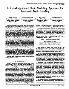
1 − wm ; (6) log(1 − w ) wm where m=n+1, Po is the probability of seeing only bad samples (in our experiments it was up to 80% for some data sets), w – probability of good (inlier) samples. The detection results were visually evaluated in 77 T2 STIR and 5 HASTE images from different hospitals. Results appeared satisfactory in all images. Segmentation accuracy was numerically evaluated using manually segmented ground truth (GT) in 35 T2 STIR images with average voxel size of 1.25x1.25x6mm. The average segmentation accuracy, estimated as ratio of overlapping of automatically detected (AD) and GT spinal cord volumes to the GT volume, was 91% with standard deviation (STD) of 14%. The accuracy of centerline position evaluated as average distance from all GT spinal cord voxels to the AD centerline was 4.4mm with STD of 1.9mm. The presence of collapsed vertebrae and edema in 1 patient (see Fig. 1) and multiple vertebrae metastasis in 12 patients did not affect the segmentation accuracy in all cases but one, where all vertebrae had severe metastatic changes of similar image intensity as spinal cord with no visible boundary. As a result spinal cord centerline was shifted toward the center of the vertebral body. k =

log( Po )

m

+

a) b) Fig. 1. a). Spinal cord detection result shown in a maximum intensity projection image of a patient with collapsed vertebrae and edema. b) Curved MPR view of vertebrae column of another patient with several metastatic lesions. Curved MPR view was computed based on detected spinal cord.

3 Parametric model based vertebrae segmentation Our vertebrae model is aimed to fit only the vertebrae body, excluding the processes and pedicles. It can be represented by a section of a curved cylinder adjacent to the spinal cord. The main motivations for this model are as follows. First, metastases that are present only in the pedicles but not vertebrae body are very rare and, second, processes and pedicles are not distinctly visible at the resolutions with slice thickness of ~6mm that are common for metastases screening protocols. On the other hand, when higher resolution screening images are available, vertebrae segmentation algorithm described in this paper can be used for rough vertebrae location at reduced resolution (sub-sampled images) and then other methods can be applied for refined vertebrae segmentation.

Median intensity

We assume that imaginary planes that separate vertebrae from each other and from inter-vertebrae disks are orthogonal to the spinal cord (see Fig. 2). projected signal min rank filtered signal band-pass filtered signal

Visible disks

t

Fig. 2. Plot of projected median intensity along spinal cord and filtered signal.

Vertebrae separating planes are detected by analyzing the one-dimensional signal representing the spinal column. The signal is extracted by projecting the median intensity values along the spinal cord inside the small sample circles adjacent to the front edge of the spinal cord within the planes orthogonal to it. Normal vertebra is composed of spongy bone, containing bone marrow, which is surrounded by compact (cortical) bone. The most interesting property of cortical bone from MRI point of view is that it does not generate signal in MRI and therefore appears consistently hypointense in any pulse sequence, while vertebra and disks may change their appearance depending on the presences of metastases or other diseases (sometimes inter-vertebrae disks are not visible in the whole vertebral column). To extract reliable information from the projected signal and skip inconsistent high intensity peaks like disks and lesions, we apply minimum rank filter with the width between the largest inter-vertebra space and shortest vertebrae that we want to detect. Next, band-pass filtering with frequency band derived from the height range of normal vertebrae body is applied to determine vertical vertebrae boundaries.

While different band of frequencies (or height thresholds) could be used in cervical, thoracic and lumbar areas for higher precision, in the current implementation we used the same band for the whole vertebrae column. Discrete Fourier transform (DFT) of the input signal is computed with a fast Fourier transform algorithm. Next, we set all the elements of the resulting vector Y to zero, which correspond to the frequencies outside of desired range. Finally, inverse Fourier transform f(y) is obtained from the vector Y. The advantage of the filtered signal is that it is smooth, therefore differentiable. It is easy to find local minimums and maximums in this signal; minimums correspond to inter-vertebrae spaces and maximums to vertebrae body. Local maximums f(mi) and minimums f(ni)of filtered signal are computed from: ∂f ∂2 f ∂f ∂2 f = 0; 2 < 0; f ( y ) > 0; f (mi ); = 0; 2 > 0; f ( y ) < 0; f (ni ); (7) ∂y ∂y ∂y ∂y where y is the distance along spinal cord. Then the precise locations of lower and upper boundary of each vertebra are found from the original signal, as two local minima f(ui) and f(di) around the middle of each vertebra mi, which represent the upper and lower boundary of each vertebra. The local minima that are caused by noise are removed by setting the adaptive amplitude threshold ti for each vertebra: f (ui ) < ti ; f ( d i ) < ti ; where ti = mean( f ( n1 − 1 ),..., f (ni + 1 )) − std ( f (n1 − 1 ),..., f (ni + 1 )) . Constraints are applied to maintain minimum height of the vertebrae Tv and intervertebrae space Ts : u i − d i > Tv ; d i + 1 − u i > Ts . The next step is aimed at creating a parametric model [5] for estimating the horizontal extent of the vertebrae through fitting ellipse to the middle section of each vertebra (see Fig. 3). First, we align all training samples x based on the second extrema (thoracic curve) of the polynomial models of each spinal cord, that approximately corresponds to 8th thorasic vertebrae. We manually acquire measurements of minor b and major axis a for each vertebra though out the training set. Then, PCA is applied for all aligned and completed samples xj.

xj

=

[a j1 ,...,

a jn , b j1 ,..., b jn

]T ;

where ai – major axes (mm), bi – minor axes (mm), i=1,…,n, n is number of vertebrae, j is the sample number. Next, mean shape x is computed: x =

1 m

m j =1

m

xj;

S=

1 m

j =1

(x

j

)(

)

T

− x xj − x ;

Spk = λk pk

(8)

where m is the number of training samples, λk is kth eigenvalue, pk is kth eigenvector, k=1,..,2n and t is the number of modes. t confidence _ level 2 n λj ≥ λj ; (9) 100% j =1 j where confidence_level was set to 95%.

x = x + Pd . P=(p1,…,pt) is a matrix of t eigenvectors, d = (d1,..., dt )T is the model parameter vector. − w λ j

≤ d j ≤ w λ j , where j=1,…,t. w was set to

1. Generate new x = x + Pd .

Major axis a Minor axis b

a)

b)

Spinal cord

Vertebrae with fitted ellipse

+ +

+ + c)

Fig. 3. a). The picture of thoracic vertebra from Henry Gray’s Anatomy of the Human Body (1918). b). Schematic representation of vertebra and spinal cord. c) Axial slice through a vertebra with fitted ellipse. Locations of manually acquired reference points at the ends of major and minor axis are shown as +.

The vertebra body extent in axial planes is estimated through an ellipse-fitting

algorithm [6]. Resulting vector: x' = [a'1 ,..., a 'n , b'1 ,..., b'n ]T . Project x ′ to model space: d ' = ( x′ − x ) / P . If x’ is reasonable, d ' will satisfy

the model constraints − w λi ≤ d i ' ≤ w λi .(i=1,…,t). Otherwise bring d’ to the

range − w

λi ≤ d i '≤ w

λ i . Next, compute x = x + Pd ' .

b = ( xnew − x) / P ; − λk ≤ bk ≤ λk ;

(10)

The vertebrae segmentation algorithm was visually evaluated on 77 T2 STIR images with different levels of fat suppression and on 5 HASTE images (HASTE pulse sequence is mainly used for abdominal organs like liver). In all cases segmentation results appeared satisfactory (see Fig. 4). Although intensity distributions for majority of organs are very different for T2 STIR and HASTE images, it had no effect on the segmentation results. No changes were made to the algorithm developed originally for T2 STIR images to adapt it for the HASTE pulse sequence.

a)

b)

c)

Fig. 4. Vertebrae segmentation results for: a) Coronal T2 STIR image b). Original (left) and segmented (right) T2 STIR image with metastases. c) HASTE image.

4 Computer-aided detection of vertebrae metastases The fully automatic metastases detection algorithm (research prototype) involved primary lesion detection and false positive reduction steps. Osteoblastic metastases, unlike osteolytic, appear hypointense in STIR images, and require similar detection approach, but with inverse thresholds. Our data set does not contain enough samples of osteoblastic metastases (4 patients only) for reliable training and testing, therefore all the results and conclusions below are targeted towards osteolytic metastatic lesions. Primary lesion candidate detection inside segmented vertebrae was performed using adaptive intensity thresholds to search for any suspicious regions. Multiple features characterizing intensity, texture (moments of intensity), volume, shape (euler number, eccentricity, orientation, solidity, diameter of a circle with the same area as the region in coronal slice, orientation - the angle between the x-axis and the major axis of the ellipse that has the same second-moments as the region), and location of candidate lesions were extracted from 3D image data. Finally, a classifier constructed using the training set was applied to the candidate detections to reduce the number of false positives (FP). The classifier was constructed by taking into account the fact that a lesion may associate with several detections and if any of them is correctly classified, the lesion is considered being identified. Let m be the number of total candidates that are identified in the lesion candidate detection step, d be the number of features that are evaluated for each of the candidates. With a little abuse of notation, we use xi to denote a feature vector representation of the ith candidate. We then label the detected candidates (hits) by consulting the markers provided by expert radiologists. A candidate receives +1 label if it overlays with a lesion, or otherwise, it receives -1 label. We use C+, C- to denote the index sets that contain all candidates that are labeled +1, and -1, respectively. In the classification task, a classifier needs to be constructed based on the training sample to predict the label for any candidate detected from unseen patient data. Standard machine learning algorithms such as support vector machines (SVM), and Fisher’s linear discriminant (FLD), are often used for CAD, but our detection task has specific characteristics that cannot be employed in the standard algorithm. In particular, there can be many hits or candidate regions that refer to unique underlying malignant structure, and even if one of the hits is correctly highlighted to the

radiologist, the entire structure can be easily traced out by the radiologist. Hence correct classification of every candidate instance is not as important as the ability to detect at least one candidate that points to a malignant region. We thus formulate our problem as a problem of learning with multiple hits. We design a novel classification algorithm based on Fisher’s linear discriminant (FLD) analysis that aims to detect at least one hit for each lesion. FLD [7] has been successfully applied to many medical applications, and it fits the separation boundary between true hits and negative detections with a linear function wT x + b . Recently, FLD has been recast into an equivalent optimization problem [8] as follows: m

minimize i =1

i ∈C +

ξi 2 + γ w

ξ i = 0,

2 2

, subject to the constraints: wT xi + b = yi + ξi , i = 1, , m,

ξ i = 0, where yi denotes the label, ξi is a residual error of the

i ∈C −

model fitting, w

2 2

is the so-called regularization term that controls the classifier

complexity, and γ plays the trade-off between the residual error and the complexity regularization. Assume in total ni hits, each represented as a feature vector xij , are segmented for the ith lesion. Let

S i be the index set of all candidates pointing to the ith lesion. For

each lesion, we form a convex hull using these vectors xij in the feature space. Any point in the convex hull can be represented as a convex combination of xij , that is, j ∈ Si

λij xij , where λij ≥ 0,

λij = 1 . The goal of our learning algorithm is to

determine a decision boundary that can separate, with high accuracy, any possible part of each of the convex hulls on one side and as many as possible negative detections on the other side. It implies that we do not require the entire convex hull to correctly classified, but only any possible part of it. In other words, our algorithm solves the following optimization problem based on the FLD formulation: m

minimize i =1

wT

j ∈ Si

λij xij

ξ i 2 + γ w 2 , subject to: 2

+ b = yi + ξ i , λij ≥ 0, wT xi + b = yi + ξi , i∈C +

ξ i = 0,

∀i ∈ C − ,

ξ i = 0.

i ∈C −

λij = 1 , ∀i ∈ C + ,

(11)

The classifier obtained by solving the formulation (11) can dramatically reduce false detections in comparison with standard classification algorithms, such as FLD. Aggregation of multiple classifiers is used to get an average aggregated prediction for an unseen sample. It has been shown that the aggregation is effective on ``unstable learning algorithms where small changes in the training set result in large changes in predictions [9]. Particularly, in our case, even though FLD itself may not be so

unstable, reasonably small changes on the training sample set often cause undesirable changes on the classifier constructed due to an extremely limited size of patient data available. Hence, aggregation is necessary in order to reduce the variance of the learned classifier over various sample patient sets, thus enhancing accuracy. We carry out T trials, and in each trial, 70% of the training cases are randomly sampled, and used in the training. A linear function f t ( x) = wt T x + bt is then constructed in the trial t. The final classifier is based on the averaged model 1 T 1 T 1 T f ( x) = f t ( x) = ( wt )T x + bt . Thresholding on the value of T t =1 T t =1 T t =1 f(x) with an appropriate cut-off value a provides the final findings where a is tuned according to the desired false positive rate. If a candidate x gets f ( x ) ≥ a , then it is classified as a true hit, or otherwise it is removed from the final findings.

5 Evaluation of metastases detection algorithm The patient population included 42 patients with different histologically clarified primary tumors examined with MRI of the spine for staging and follow-up of known skeletal metastases. The gold standard was constituted by histology and/or clinical radiological follow up within at least 6 months. MRI was performed at 1.5 Tesla on a 32-channel scanner (Magnetom Avanto, Siemens). All patients underwent STIR-imaging of the complete spine in sagittal orientation. The data was split into training and test sets. Training set included 21 patients, in which 12 had osteolytic spine metastases (13 focal, 6 diffuse and 10 multifocal lesions). The test set included 21 patients, of which 9 had osteolytic spine metastases (12 focal, 6 diffuse and 8 multifocal lesions). Each spine section (cervical, thoracic and lumbar) with diffuse or multifocal infiltration was counted as one lesion. Training and test set sensitivity was 82.76% and 84.61%, respectively, with 5 false positive detections per patient. The CAD algorithm missed 3 focal lesions in the training set and 3 focal lesions in the test set. One diffuse lesion (spine section) was missed in one patient from the test set and one multifocal and one diffuse lesion were missed in two patients from the training set. However, other lesions or infiltrated spine sections were successfully detected in the same patients, so that ‘per patient’ sensitivity was 100%.

6 Conclusion Spine metastases CAD showed high standalone sensitivity at a relatively low FP rate. The run time was ~2 min on average in MATLAB implementation. While this study confirmed CAD feasibility, the next step is to incorporate additional features from T1weighted SE-sequences to further reduce the number of false positives. Furthermore, the additive benefits of CAD as a second reader should be investigated.

B A

a)

b)

c)

d)

Fig. 5. a) and b). Examples of metastases detection results on the images from the development set (coronal STIR images with less fat suppression). The left image is from the same patient with collapsed vertebrae and edema as in figure 1a. c). Test set image example: sagittal STIR image of the spine. Focal lesions detected by CAD are highlighted in red. d) ROC curves for training and test sets. A. Sensitivity at 1.5 FPs per patient: training – 66.32%, test - 61.61%. B. Sensitivity at 5.0 FPs per patient: training – 82.89%, test - 84.61%

References 1. Schmidt , G.P., Schoenberg, S.O., Schmid R, Stahl R, Tiling R., Becker C.R., Reiser, M.F. 2. 3. 4. 5. 6. 7. 8. 9.

and Baur-Melnyk, A..Screening for bone metastases: whole-body MRI using a 32-channel system versus dual-modality PET-CT. Eur Radiol. (2006) Sep 2; [Epub]. Ghanem, N., Uhl, M., Brink, I., Schäfer, O., Kelly, T., Moser, E., Langer, M. Diagnostic value of MRI in comparison to scintigraphy, PET, MS-CT and PET/CT for the detection of metastases of bone. European Journal of Radiology, Vol. 55(1), (2005) 41-55 Carballido-Gamio, J., Belongie, S., Majumdar, S. “Normalized Cuts in 3D for Spinal MRI Segmentation.” IEEE Transactions on Medical Imaging, (2004), 23(1): 36-44. Fischler, M. A., Bolles, R. C. "Random Sample Consensus: A Paradigm for Model Fitting with Applications to Image Analysis and Automated Cartography". Comm. of the ACM 24: (1981) 381-395. Cootes, T., Hill, A., Taylor, C., and Haslam, J. Use of active shape models for locating structures in medical images. Image & Vision Computing, (1994) 12(6):355-366. Saha P., Tensor scale: A local morphometric parameter with applications to computer vision and image processing, Computer Vision and Image Understanding, Volume 99, Issue 3, Pages 384-413. Johnson, R. A. and Wichern, D. W. Applied Multivariate Statistical Analysis. Prentice Hall. New Jersey. (1998). Mika, S., Ratsch, G. and Muller, K. A mathematical programming approach to the kernel Fisher algorithm. Advances in Neural Information Processing Systems. Vol.13 (2001) 591-597. Breiman, L., Bagging predictors, Machine Learning, (1996), 24(2):123-140.