We also demonstrate how our algorithm can be used to help .... issue of adapting non-rigid matching techniques to corre- ..... From the 4th and 5th sub-figure, we can observe that minimization with huber function introduces a high level of ...
2013 IEEE International Conference on Computer Vision
Robust Non-parametric Data Fitting for Correspondence Modeling Wen-Yan Lin1 1
Ming-Ming Cheng1
Oxford Brookes
2
Shuai Zheng1
Nigel Crook1
Advanced Digital Sciences Center, Singapore
Abstract
1. Introduction Fitting a warp or transformation field onto an image section is a long standing computer vision and graphics problem and lies at the heart of many novel image synthesis algorithms. While there are many techniques for establishing correspondence between images [24, 23, 13], converting them into a coherent warp remains a significant problem. For specific applications or correspondence types, there have been many proposals regarding how outlying correspondence can be removed [31] or correspondence jointly estimated with the warp [21]. What is lacking is a generic, computationally simple method to robustly establish a nonparametric warp from noisy correspondence. To date the most commonly used generic techniques for fitting warps to correspondences take the form of rigid affine or homographic transforms. These warps are parametric, with the small parameter size providing robustness to noise and outliers. While parametric techniques are very robust, many real world scenarios involve complex motions that would benefit from less restrictive parameterization. We pose this warping problem as a data fitting question: How is it possible to robustly compute a non-parametric fitting function across noisy scatter points? ”The direct fitting of a fully flexible non-parametric function would almost certainly result in difficulties defining and removing outliers. This would be especially dif-
Warping Results
Overlays Results
SIFT flow
Target
Inputs
Our SIFT Flow Refinement
Source
We propose a generic method for obtaining nonparametric image warps from noisy point correspondences. Our formulation integrates a huber function into a motion coherence framework. This makes our fitting function especially robust to piecewise correspondence noise (where an image section is consistently mismatched). By utilizing over parameterized curves, we can generate realistic nonparametric image warps from very noisy correspondence. We also demonstrate how our algorithm can be used to help stitch images taken from a panning camera by warping the images onto a virtual push-broom camera imaging plane.
1550-5499/13 $31.00 © 2013 Crown Copyright DOI 10.1109/ICCV.2013.295
Jiangbo Lu2
Homography SIFT Flow Refinement
Figure 1. Our algorithm can fit a smooth surface to noisy SIFT flow correspondences [23], allowing a visually pleasing warp.
ficult for piece-wise outlier corruption where certain image sections are consistently matched incorrectly. However, we note that by including an additional constraint requiring data to form a smooth curve, outliers (especially piece-wise outliers) can then be readily defined. While loosing some modeling flexibility, such a scheme has the potential to provide a level of robustness similar to parametric affine and homographic fitting while providing significantly greater flexibility. We propose a non-parametric function fitting approach that is based upon the motion coherence formulation discussed by Yuille and Grywacz [41], Myronenko et al. [28]. We observe that the original proofs based upon L2 correspondence fitting can be adapted to a robust huber loss function. The resultant formulation computes a smooth, best fit curve for a noisy point set by minimizing a simple convex cost. With a simple Median Absolute Deviation thresholding to replace the RANSAC [11], our proposed algorithm’s enforcement of overall smoothness makes it especially adept at handling piece-wise noise in which certain data sections are corrupted in a coherent manner. When we integrate our 1-dimensional curve fitting into the over parametrized warping scheme proposed by Lin et al., Nir et al. [22, 29], we can compute coherent warps from noisy image correspondences. Figure 1 illustrates our warping technique. 2376
As our warping technique is defined in terms of nonparametric curve fitting, rather than correspondence reestimation, it lends itself naturally to image re-projection problems. In particular, it allows orthographic image projection from noisy depth estimates. This is especially useful for mosaicking long lateral image sequences taken by a panning camera. To summarize, our contributions are as follows: • We propose a non-parametric curve fitting technique that is robust to piecewise noise. • We incorporate the technique into a high dimensional smoothly varying warping scheme that allows computation of visually compelling image warps from noisy correspondence in a simple minimization framework. • We demonstrate a panning mosaicking algorithm that integrates images from a laterally translating camera by stitching them to a push-broom mosaicking plane.
2. Related Works Non-parametric data fitting and its associated image warping is a large and well researched computer vision field. Works range from self occlusion surface fitting [31], full frame internet image warping [21], bio-medical contour registration [28], non-rigid surface reconstruction [36, 34], as-rigid-as-possible shape manipulation [18] and non-rigid 3-D object warping [39]. Non-rigid fitting also encompasses the wide range of flow based works, [23, 25, 17, 6] and piecewise segment fitting techniques [3, 37]. However, most works focus on custom applications to specific problems and their adaptation to a generic non-parametric correspondence fitting scheme is unclear since they integrate many different aspects (matching cost, descriptor information and smoothness term) within a single system. The issue of adapting non-rigid matching techniques to correspondence fitting is considered in the subsequent paragraph. Non-rigid correspondence estimation algorithms such as Chui et al. for thin-plate spline [8], Wills et al. in mixed optical flow, thin-plate spline computation [40], Myronenko et al. in motion coherence [28] and Lin et al. in smoothly varying affine [22], iteratively compute a smooth warping surface and do not assume known correspondences. These formulations can also be readily adapted from correspondence discovery to the simpler correspondence fitting problem by redefining the matching choices into a binary match or no-match decision. Our approach is inspired by this line of reasoning. However, we note that if the task is simply to decide between a match and non-match, we can eliminate the complex iterative correspondence estimation procedure that is vulnerable to local minimums. In this paper, we adapt the motion coherence formulation [28] such that
B
A : outliers C
Figure 2. While the outlier points in B can be potentially fitted using a spline, their outlier status becomes much less ambiguous if we define the problem as a smooth curve fitting.
the matching cost is penalized with a simple huber function. This adaptation allows a simple convex cost that can be minimized to find the desired warping field. Our work also bears close relation to spline fitting techniques such as Reinsch [35], Akima [2], Garcia [15]. Unlike spline fitting, we require our fitted function to be a smooth curve. This is less flexible than a spline, but it allows the fitting of a trend through piece-wise outlier corruption. This is illustrated in Figure 2,4.
3. Formulation We pose the correspondence modeling problem as one of robust non-parametric curve fitting. Traditionally, nonparametric function estimation is viewed as more unstable than its parametrized cousin. We feel that this is in large part due to the difficulty in defining noise and outliers in a non-parametric setting. In particular piece-wise noise in which a section of the signal is corrupted consistently can be difficult to handle. However, by reducing the non-parametric space to a smaller one consisting of smooth continuous functions, such outliers can be well defined as illustrated in Figure 2. As such, we propose a non-parametric curve fitting that is robust to piecewise corruption and extend our results to the creation of smooth warps from noisy correspondences. Our proposed solution can provide high stability levels usually only associated with parametric algorithms.
3.1. Using Motion Coherence to formulate a function fitting problem The problem is formulated as the fitting of a smooth function to data. Given a set of N scatter points {pj , qˆj }, where pj are D-dimensional vectors and qˆj are scalars. We assume that data comes from a linear combination of K smooth functions fk (p), corrupted with noise. Thus, qˆj =
K � k=1
2377
ajk fk (pj ) + nj .
(1)
nj represents noise and ajk are given weight values for the linear combination of fk (.) functions. Individual fk (.) functions are composed of two terms, fk (p) = Hk + φk (p). Hk is a scalar offset and φk (p) is a smooth function with motion coherence smoothness penalty [41, 28] given as follows � Ψk =
RD
|φk (ω)|2 dω. g(ω)
(2)
φk (.) denotes the Fourier transform of a function φk (.), while g(ω) is the Fourier transform of a Gaussian with spatial distribution γ. Hence, Eqn. (2) achieves smoothness by penalizing high frequency terms. Our goal is to find the smoothest possible fk (.) functions consistent with the given {pj , qˆj } data points. This is expressed as the energy E=
N � j=1
C(ˆ qj −
K �
ajk fk (pj )) + λ
k=1
K �
Ψk
(3)
k=1
Here, C(.) represents some cost function that penalizes deviation of the estimated function predictions from given qˆ estimates. Throughout this paper, we use the huber function in Eqn. (9), though other functions are possible. λ represents the weight given to the smoothness constraint Ψk . The cost E can be re-expressed in terms of a finite number of wk , Hk using Eqn. (6) and (7), thus allowing minimization. We discuss in the procedure in following paragraphs. Directly minimizing E with respect to functions fk (.) appears intractable as the minimization occurs over continuous functions. However, motion coherence can reduce the problem to an optimization over a finite number of variables. A brief summary is as follows: Fourier transform relation, φk (p) = � Note the2πι φ (ω)e dω. Considering E of Eqn. (3), we D k R know that at the minima, its derivative is zero. Hence, δE = 0, ∀z ∈ RD , k ∈ {1, 2, ..., K} δφk (z) =>
N �
wk (j)e2πι + 2λ
j=1
φk (−z) =0 g(z)
vectors, φk (p) =
N �
wk (j)g(p − pj , γ).
(6) Similarly, substituting (5) into (2), the continuous regularization function can also be expressed in terms of wk Ψk = wkT Gwk ,
N �
wk (j)e−2πι
k ∈ {1, 2, ..., K}
(7)
where G is a symmetric matrix with G(i, j) = g(pi − pj , γ) = e−|pi −pj |
2
/γ 2
(8)
Substituting Eqn. (6) and (7) into (3), the energy is dependent only on a finite number wk and Hk variables and can be minimzed accordingly. We make a few observations. First, the formulation accommodates a wide range of cost functions C(.) in Eqn. (3). The only requirement is the function must be continuously differentiable. Second, as G is a Gram matrix [28], the coherence term Ψk in Eqn. (7) is convex. The sum of convex functions remains convex. Thus, choosing a convex cost function for C(.) (such as huber or L2 norm) will mean the overall energy minimization problem is convex. In this paper, we set C(.) to be the huber function: � 2 z if z ≤ � C(z) = huber(z) = (9) 2�|z|1 − �2 if z > �
3.2. 1-Dimensional curve fitting As an introduction, we apply the formulation to a 1dimensional curve fitting problem. This is a K = 1, D = 1, ajk = 1 case of Eqn. (3). As K = 1, we drop the k subscript from notations. The given, set of N data points{pj , qˆj }, are noisy observations of a single smooth function f (p), with Eqn. (1) reducing to qˆj = f (pj ) + nj . nj represents noise, while f (p) takes the form f (p) = H + φ(p)
(4)
(10)
where φ(p) has smoothness penalty � Ψ=
Making some minor rearrangement we have φk (z) = g(−z)
k ∈ {1, 2, 1..., K}
j=1
(5)
j=1
where wk are N × 1 vectors that serve as place-holders for more complicated terms. Taking the inverse Fourier transform of eqn (5), we can write our continuous functions in terms of a finite set of wk
R
|φ(ω)|2 dω. g(ω)
(11)
Following Eqn. (3), with C(.) set to the huber function given in Eqn. (9), we can express the search for a smoothest possible f (p), consistent with the given {pj , qˆj } scatter plot through a robust energy function, E=
N � j=1
2378
huber(ˆ qj − f (pj )) + λΨ
(12)
This gives the overall cost
From Eqn. (6) and (7) we can re-parameterize the continuous functions φ(p), Ψ with finite variables: �N
φ(p) =
j=1
w(j)g(p − pj , γ),
T
Ψ = w Gw,
(13)
where G is defined in Eqn. (8). Substituting these into Eqn. (10), and (12), we re-express the continuous function f (p) and energy cost E=
N �
Ex =
huber (ˆ qj − H − φ(pj )) + λwT Gw
j=1
fk (p) = Hk + Ex =
N �
(18)
wk (j)g(p − pj , γ), k ∈ {1, 2, 3}
yj� ]}.
f1 (p)x + f2 (p)y + f3 (p) . H4 x + H5 y + 1
f6 (p)x + f7 (p)y + f8 (p) , H9 x + H10 y + 1 cy (pj ) =(yj� )(H9 xj + H10 yj + 1) − (f5 (pj )xj + f6 (pj )yj + f7 (pj ))
We handle the denominator’s non-linearity in Eqn. (14) by multiplying it out to give a linearized penalty cx (pj ) =(x�j )(H4 xj + H5 yj + 1) (17)
This penalty is a K = 5 case of Eqn. (3) by dropping φk (.) (or setting its coherence penalty to infinity) terms for f4 (.), f5 (.), setting qˆj to zero and choosing the appropriate ajk values. For example a1,1 = x1 , a20,4 = −x�20 x20 .
(19)
(20)
(21)
Similar to the process for x� , we can solve for the fk (.), k ∈ {6, 7, 8} functions by re-parameterizing the functions and penalty cost in terms of Hk and wk vectors of the form N �
wk (j)g(p − pj , γ), k ∈ {6, 7, 8}
j=1
(14)
with Hk being scalar unknowns and φk having smoothing constraint � |φk (ω)|2 Ψk = dω. (16) g(ω) R2
wkT Gwk .
k=1
fk (p) = Hk +
(15)
3 �
y� =
Ey =
The fk : R → R functions can be considered locally varying affine parameters and take the form
− (f1 (pj )xj + f2 (pj )yj + f3 (pj )).
huber(cx (pj )) + λ
For the y � , we adopt a similar formulation to the x� values in Eqn. (14). This gives a penalty functions
2
fk (p) = Hk + φk (p),
N � j=1
xj , yj are image coordinates in the first image and x�i , yj� are their correspondence in the second image. Our goal is to fit a smooth transform that maps coordinates from the first image to the second. We begin by focusing on the mapping of xj , yj to x�j . With reference to the general formulation in Section 3.1, the input function domain is p2×1 = [ x y ]T . In this paper, we utilize a smoothly varying quasihomographic transform. In it the motion is assumed to be modeled by a global homography with some local variations, an approach similar to that of [22]. Formally, the relation is given by x� =
Ψk ,
k=1
j=1
We denote the given set of N matches as x�j ;
3 �
where the huber function is defined in Eqn. (9). From Eqn. (6) and (7) we can reduce the continuous functions φk (p), Ψk to a parameterization with finite variables. Substituting Eqn. (6) and (7) into (15), and (18), re-expresses the continuous function fk (p) and cost Ex in terms of a finite number of variables, Hk , wk . This gives:
3.3. Fitting image correspondence yj ;
huber(cx (pj )) + λ
j=1
in terms of a finite number of variables, i.e. H and wN ×1 . As argued in Section 3.1, the function E is convex.
{mj = [ xj ;
N �
N �
huber(cy (pj )) + λ
j=1
8 �
wkT Gwk
(22)
k=6
and minimizing energy Ey . As argued in Section 3.1, the energies Ex , Ey are convex.
3.4. Implementation Although the cost is convex, good initialization improves efficiency. For initialization, we solve Eqn. (3) with � in Eqn. (9) set to infinity. This makes the cost a sum of squares (recall, G is a Gram matrix) and provides the initialization for the gradient descent minimization of Eqn. (3),(12),(19),(22). While simple minimization of the cost produces good results, we find further quality improvements arise from iterative thresholding. After each solution, we remove as outliers, points whose deviation from the curve is 1.48 times the Median Absolute Deviation (MAD) (threshold assuming Gaussian noise). The curve is 2379
re-computed using the inlier points and the process repeated 3 times. We term this scheme MAD thresholding. This replaces RANSAC [12] used in parametric formulation. An empirical analysis of its impact is offered in Figure 5.
4. Non-parametric Curve Fitting Evaluation We undertake quantitative evaluation of our basic formulation in Section 3.2. This is the curve fitting problems of the form q = f (p). p-coordinates √ are normalized to mean zero and mean absolute value 1/ 2. q-coordinates are normalized to zero mean and mean absolute value 0.0001 (this value is deliberately small to reduce the coherence penalization of low frequency terms). γ, λ, � are set to 1, 0.01, 0.1 × 0.0001 respectively. We minimize Eqn. (12) with 3 iterations of MAD thresholding. This setting is referred to in Figures 3, 4, 5 as Ours Default. For evaluation, we add noise to points from pre-defined functions. Each point is corrupted with Gaussian noise of standard deviation equal to 5% of the maximum function deviation (max(f (p))−min(f (p))). We also randomly corrupt 6% of the points with point wise outliers and 13% with piece-wise outliers. In Figure 3, we estimate the original function using Ours Default. For comparison, we also applied the robust spline implementation in [26] (which we tuned for good performance, among the parameters tested was the cubic spline which is the thin-plate spline’s 1D analogue) and Adaptive Fitting for Gridded Data [15]. Figure 3 provides residual RMSE error and its percentage relative to the original noise. Our technique achieves low noise values under difficult evaluation conditions. A visual relation between errors and accuracy is provided in figure 4. Note that while our algorithm is especially adept at handling piece-wise noise, we do not claim it is an intrinsically better spline fitting technique for all circumstances, since the definition of a good fit depends on the definition of noise. Functions
Ours (default) 0.33 16% 1.0 16% 0.077 15% 0.074 18%
Spline Robust 1.47 75% 3.3 46% 0.43 89% 0.34 82%
Spline Adaptive 1.35 68% 4.7 67% 0.3 63% 0.27 66%
Figure 3. Without knowing the underlying function, we try to estimate the curves on the left from noisy point estimates. Tabulated results show average RMSE over 100 iterations and the RMSE as a percentage of added noise. Baseline comparison against robust spline fitting [26] and adaptive spline fitting [15] show our error ( 16−18%) is significantly lower than other techniques ( 63−89%). Visualization is provided in Figure 4.
Figure 5, illustrates the impact of various aspects of our
algorithm. We compare direct minimization of huber cost without MAD thresholding (Single iteration, huber) with minimization of an L2 norm (Single iteration, no huber). The huber function provides a marked increase in stability (in our experiments, the average improvement is 140%). We also compare the huber cost function with MAD thresholding (Ours Default) against the L2 norm with MAD thresholding (3 iterations no huber). MAD thresholding reduces the difference between huber and L2 norm, but the huber based technique still retains an average 32% improvement.
5. Image Correspondence We also apply our algorithm on noisy correspondence between real images. We consider two cases. The first involves extracting a warp from a SIFT flow field while the second involves a mosaicking application. Both cases utilize the same control variables. The point coordinates are normalized using Hartley normalization [16]. Point set are defined as the centroids of mean shift [9] segments. λ, γ and � parameters are set to 100, 1 and 0.01 respectively. Further, the motion field is scaled so that the maximum deviation between motion values is capped at 0.01.
5.1. SIFT flow One can utilize SIFT flow [23] to compute correspondence relationships between very different images. However, the resultant warps are often visually corrupted. Our technique can fit a smooth motion field over such warps, allowing substantial improvement in viusla quality, while adhering to the SIFT flow defined motion. This is illustrated in Figures 1 and 6. Note that our algorithm seeks to follow the SIFT flow field which may or may not correspond to the correct warp between images. Thus, for the horse image in the second row, while the result does not correspond closely to the target image, it does relate well to the original SIFT flow field. Our algorithm gives good adherence to the SIFT flow field as can be seen from the shadowing in Figure 6, while having reduced distortion compared to thin-plate spline. For example, in the temple image, our technique incurs less bending at the building eves, while for the horse man, we could shrink the rider in accordance with SIFT flow, while still preserving the straight sword. This can be seen in the reduced shadowing. These results can be useful in graphics applications such as [20, 7]. We acknowledge the limitations to such visual comparisons which unlike curve fitting discussed in the previous section, does not lend itself well to numerical analysis. Further, there remain bending artifacts which are visually displeasing.
5.2. Panoramas from panning camera Creating panoramas by image mosaicking is a common warping application. This can be achieve through both parametric [5, 27, 1] and non-parametric [22, 14] approaches 2380
Figure 4. Visualization of curves estimated from data. Error is RMSE as a percentage of the added noise. Robust Spline is the tuned spline fit implementation [26]. Adaptive Spline refers Garcia’s [15] algorithm. Note our approach’s immunity to piece-wise outliers.
Figure 5. Effects of huber function and MAD thresholding. From left to right: 1) Original curve. 2) Our’s default: Huber cost with MAD thresholding. 3) 3 iterations, no huber: L2 norm with MAD thresholding. 4) Single iteration, huber: Minimization of huber cost, with no MAD thresholding 5) Single iteration, no huber L2 norm with no MAD thresholding. RMSE is given as a percentage of the added noise. From the 4th and 5th sub-figure, we can observe that minimization with huber function introduces a high level of stability. This carries over to the 2nd and 3rd sub-figures, where despite MAD thresholding, the huber solution is still better. Overall statistics for the curves in Figure 3, show that (Our’s default) has a 32% improvement over (3 iterations, no huber), while (Single iteration, huber) has a 140% improvement over (Single iteration, no huber). Input
SIFT flow initialization
Ours
Thin Plate Spline
Translation
Homography
Mosaicking plane
x y
Orthographic axis
Perspective axis Virtual slit camera
Mosaicking plane Translation projection Camera trajectory
Figure 7. Top: Illustrates a push-broom camera system, which images perspective slices as a single pixel width camera translates in a straight line. Bottom: We project our image sequence points onto a virtual push-broom imaging plane to create a mosaic, with each image mapping to a small section of the push-broom mosaic. Note that the re-projection parallax induced by such a warping is limited since each image is only re-projected a small distance from its original position.
Figure 6. Refining a SIFT flow warping field. Warping results are overlaid onto the original SIFT flow projection by replacing the SIFT flow warps green channel. Our algorithm gives close adherence to the original SIFT flow field as indicated by the small amount of shadowing present in the overlay. However, the results are visually much better compared to the original SIFT flow.
that warp images to a central frame. While such approaches work well under low parallax conditions, the algorithms are not designed for handling long, panning camera motions. This section explains how our warping technique can be integrated into a geometric re-projection scheme to create
panning mosaics. The basic problem is as follows. Assume a base frame at world coordinates (0, 0, 0), to which we seek to project 2381
all images, taken by a camera panning in the X direction. For an image pixel location pj which corresponds to 3-D point [ Xj Yj Zj ]T , its projection to the base frame is lj = [ Xj /Zj Yj /Zj ]T . As Xj increase with camera pan, the influence of Zj grows, amplifying the parallax induced by depth differences. The growing parallax introduces large motion discontinuities that cannot through warping schemes that impose coherent motion. Rather than warping to a base frame, we warp to a virtual push-broom camera projection plane. Thus pj is projected onto mosaic position lj = [ sXj
Yj /Zj ]T = [ x�j
Input Sequences
Ours
yj� ]T ,
where s is a given constant. This definition of a warp form bj to x� , y � can be modeled with a smoothly varying field. The field can then be solved through minimization of Eqn. (19), (22) to obtain the Hk , wk warping parameters, which will project each image pixel onto the mosaic using Eqn. (14), (20). From Figure 7 we can see that for a camera panning in the X direction, this formulation de-couples the relation between induced parallax and X coordinate as each camera re-projects onto a nearby frame. This approach is similar to the strip cutting techniques of Qi et al. [32] and Dornaika et al.[10] which rely on 3-D reconstruction to create a virtual ‘video’ of a camera translating uniformly in a single direction. The central strip of each video still are then merged [33, 19]. While we are also dependent on 3-D reconstruction to recover camera positions [38] and some sparse 3-D projections [13], our technique allows projection of overlapping images onto the mosaicking plane. This permits implementation of the Poisson blending [30] and seam finding [4] to handle inconsistencies. This makes our technique less dependent on stereo quality which can be brittle. The left image in Figure 8 contains a room scene with strong parallax. This fails non-rigid warping techniques [21]. The room also contains complex structures such as the chair, and multiple occlusion boundaries that make it difficult to mosaic directly from 3-D information. Observe that our technique correctly compressed the fore-ground to allow merging of images. The drawback of our algorithm is bending that occurs about the mosaic boundary. This occurs because there is little 3-D information for the end frames and the algorithm is forced to extrapolate. In contrast, pure homographic techniques like [5],[27],[1], create warps that do not share a common joining boundary. This induces error when merging images. The right image in Figure 8, shows a substantially longer sequence of 28 images. Our algorithm can merge all these images into a single panning mosaic, illustrating the strength of the mixed geometric and warping technique.
Auto-stitch
I2k Align
Aligning Images in the Wild
Microsoft ICE
Figure 8. Mosaics creating by panning a camera in the X-direction. The results are shown for Ours, Auto-Stitch [5], I2K [1], Aligning Images in the Wild [21] and Microsoft ICE [27]
6. Conclusion We propose a technique that can robustly fit a smooth non-parametric curve to data that contains piece-wise signal corruption. We demonstrate how this technique extends to smoothly varying models that fit image correspondences. While explicitly over smoothing the data, our algorithm can handle very high noise levels within a simple minimization framework. Its primary draw-back is its lack of straight line preservation and the occurrence of bending artifacts near 2382
image edges or when there is insufficient data to guide the algorithm. Acknowledgments: We thank the ICCV reviewers for many suggestions for improving the paper. We also thank Philip Torr for allowing us the time to investigate this topic and are grateful for the support of EPSRC grant EP/I001107/1. Jiangbo Lu acknowledges the HSSP research grant at the ADSC from Singapore’s Agency for Science, Technology and Research (A*STAR).
References [1] Dual align. http://www.dualalign.com, 2010. [2] H. Akima. A new method of interpolation and smooth curve fitting based on local procedures. J.ACM, 1970. [3] P. Bhat, K. C. Zheng, N. Snavely, and A. Agarwala. Piecewise image registeration in the presence of multiple large motions. CVPR, 2006. [4] Y. Boykov and V. Kolmogorov. An experimental comparison of min-cut/max-flow algorithms for energy minimization in vision. IEEE Trans. Pattern Anal. Mach. Intell, 2004. [5] M. Brown and D. Lowe. Automatic panoramic image stitching using invariant features. IJCV, 1(74):59–73, 2007. [6] T. Brox, A. Bruhn, N. Papenberg, and J. Weickert. High accuracy optical flow estimation based on a theory for warping. ECCV, pages 25–36, 2004. [7] T. Chen, M.-M. Cheng, P. Tan, A. Shamir, and S.-M. Hu. Sketch2photo: Internet image montage. SIGGRAPH Asia, 2008. [8] H. Chui and A. Rangarajan. A new algorithm for non-rigid point matching. In Proc. of Computer Vision and Pattern Recognition, 2000. [9] D. Comaniciu and P. Meer. Mean shift: A robust approach toward feature space analysis. IEEE Trans. Pattern Anal. Mach. Intell., 24(5):603–619, 2002. [10] F. Dornaika and R. Chung. Mosaicking images with parallax. Signal Processing: Image Communication, 2004. [11] M. A. Fischler and R. C. Bolles. Random sample consensus: A paradigm for model fitting with applications to image analysis and automated cartography. Comm. of the ACM, 24:381–395, 1981. [12] M. A. Fischler and R. C. Bolles. Random sample consensus: A paradigm for model fitting with applications to image analysis and automated cartography. Comm. of the ACM, 24:381–395, 1981. [13] Y. Furukawa and J. Ponce. Accurate, dense, and robust multiview stereopsis. IEEE Transactions on Pattern Analysis and Machine Intelligence, 2010. [14] J. Gao, S. J. Kim, and M. S. Brown. Constructing image panoramas using dual-homography warping. CVPR, 2011. [15] D. Garcia. Robust smoothing of gridded data in one and higher dimensions with missing values. Computational Statistics and Data Analysis, 2010. [16] R. I. Hartley. In defense of the eight-point algorithm. IEEE Trans. Pattern Analysis and Machine Intelligence, 19(6):580–593, 1997. [17] B. Horn and B. Schunck. Determining optical flow. Artificial Intelligence, 1981.
[18] T. Igarashi, T. Moscovich, and J. F. Hughes. As-rigid-aspossible shape manipulation. ACM Trans. Graph., 24:1134– 1141, July 2005. [19] J. Kopf, B. Chen, R. Szeliski, and M. Cohen. Street slide: Browsing street level imagery. ACM Trans. Graph., 2010. [20] J.-F. Lalonde, D. Hoiem, A. A. Efros, C. Rother, J. Winn, and A. Criminisi. Photo clip art. SIGGRAPH, 2007. [21] W.-Y. Lin, L. Liu, Y. Matsushita, K.-L. Low, and S. Liu. Aligning images in the wild. CVPR, 2012. [22] W.-Y. Lin, S. Liu, Y. Matsushita, T.-T. Ng, and L.-F. Cheong. Smoothly varying affine stitching. CVPR, 2011. [23] C. Liu, J. Yue, A. Torralba, J. Sivic, and W. T. Freeman. Sift flow: Dense correspondence across different scenes. ECCV, 2008. [24] D. G. Lowe. Distinctive image features from scale-invariant keypoints. IJCV, 60(2):91–110, 2004. [25] B. Lucas and T. Kanade. An iterative image registration technique with an application to stereo vision. Proceedings of Imaging understanding workshop, 1981. [26] J. Lundgren. Robust splines. www.mathworks. co.uk/matlabcentral/fileexchange/ 13812-splinefit, 2011. [27] Microsoft. Microsoft image composite editior. 2011. [28] A. Myronenko, X. Song, and M. Carreira-Perpinan. Nonrigid point set registration: Coherent point drift. NIPS, 2007. [29] T. Nir, A. M. Bruckstein, and R. Kimmel. Overparameterized variational optical flow. IJCV, 2007. [30] P. P´erez, M. Gangnet, and A. Blake. Poisson image editing. SIGGRAPH, 2003. [31] D. Pizarro and A. Bartol. Feature-based deformable surface detection with self-occlusion reasoning. IJCV, 2012. [32] Z. Qi and J. Cooperstock. Overcoming parallax and sampling density issues in image mosaicing of non-planar scenes. BMVC, 2007. [33] A. Rav-Acha, Y. Shor, and S. Peleg. Mosaicing with parallax using time warping. Computer Vision and Pattern Recognition Workshop, 2004. [34] L. A. Ravi Garg, Anastasios Roussos. A variational formulation for dense non rigid structure from motion. CVPR, 2013. [35] C. H. Reinsch. Smoothing by spline functions. Numerische Mathematik, 1967. [36] A. Roussos, R. G. Chris Russell, and L. Agapito. Dense multibody motion estimation and reconstruction from a handheld camera. ISMAR, 2012. [37] S. N. Sinha, D. Steedly, N. Snavely, and R. Szeliski. Piecewise planar stereo for image-based rendering. CVPR, 2006. [38] N. Snavely, S. M. Seitz, and R. Szeliski. Modeling the world from internet photo collections. International Journal of Computer Vision, 2007. [39] R. Szeliski and S. Lavallee. Matching 3-d anatomical surfaces with non-rigid deformations using octree splines. IJCV, 1996. [40] J. Wills and S. Belongiei. A feature-based approach for determining dense long range correspondences. ECCV, 2004. [41] A. L. Yuille and N. M. Grywacz. The motion coherence theory. ICCV, 1988.
2383