Robust Semantic Text Similarity Using LSA, Machine Learning, and ...

Language Resources and Evaluation: Preprint Final publication is available at Springer via http://dx.doi.org/10.1007/s10579-015-9319-2

Robust Semantic Text Similarity Using LSA, Machine Learning, and Linguistic Resources Abhay Kashyap · Lushan Han · Roberto Yus · Jennifer Sleeman · Taneeya Satyapanich · Sunil Gandhi · Tim Finin

Received: 2014-11-09 / Accepted: 2015-10-19

Abstract Semantic textual similarity is a measure of the degree of semantic equivalence between two pieces of text. We describe the SemSim system and its performance in the *SEM 2013 and SemEval-2014 tasks on semantic textual similarity. At the core of our system lies a robust distributional word similarity component that combines Latent Semantic Analysis and machine learning augmented with data from several linguistic resources. We used a simple term alignment algorithm to handle longer pieces of text. Additional wrappers and resources were used to handle task specific challenges that include processing Spanish text, comparing text sequences of di↵erent lengths, handling informal words and phrases, and matching words with sense definitions. In the *SEM 2013 task on Semantic Textual Similarity, our best performing system ranked first among the 89 submitted runs. In the SemEval-2014 task on Multilingual Semantic Textual Similarity, we ranked a close second in both the English and Spanish subtasks. In the SemEval2014 task on Cross–Level Semantic Similarity, we ranked first in Sentence–Phrase, Phrase–Word, and Word–Sense subtasks and second in the Paragraph–Sentence subtask. Keywords Latent Semantic Analysis · WordNet · term alignment · semantic similarity 1 Introduction Semantic Textual Similarity (STS) is a measure of how close the meanings of two text sequences are [4]. Computing STS has been a research subject in natural language processing, information retrieval, and artificial intelligence for many years. Previous e↵orts have focused on comparing two long texts (e.g., for document classification) or a short text with a long one (e.g., a search query and a document), but there are a growing number of tasks that require computing Abhay Kashyap, Lushan Han, Jennifer Sleeman, Taneeya Satyapanich, Sunil Gandhi, and Tim Finin, University of Maryland, Baltimore County (USA), E-mail: {abhay1, lushan1, jsleem1, taneeya1, sunilga1, finin}@umbc.edu; Roberto Yus, University of Zaragoza (Spain), E-mail: [email protected]

2

Abhay Kashyap et al.

the semantic similarity between two sentences or other short text sequences. For example, paraphrase recognition [15], tweets search [49], image retrieval by captions [11], query reformulation [38], automatic machine translation evaluation [30], and schema matching [21, 19, 22], can benefit from STS techniques. There are three predominant approaches to computing short text similarity. The first uses information retrieval’s vector space model [36] in which each piece of text is modeled as a “bag of words” and represented as a sparse vector of word counts. The similarity between two texts is then computed as the cosine similarity of their vectors. A variation on this approach leverages web search results (e.g., snippets) to provide context for the short texts and enrich their vectors using the words in the snippets [47]. The second approach is based on the assumption that if two sentences or other short text sequences are semantically equivalent, we should be able to align their words or expressions by meaning. The alignment quality can serve as a similarity measure. This technique typically pairs words from the two texts by maximizing the summation of the semantic similarity of the resulting pairs [40]. The third approach combines di↵erent measures and features using machine learning models. Lexical, semantic, and syntactic features are computed for the texts using a variety of resources and supplied to a classifier, which assigns weights to the features by fitting the model to training data [48]. In this paper we describe SemSim, our semantic textual similarity system. Our approach uses a powerful semantic word similarity model based on a combination of latent semantic analysis (LSA) [14, 31] and knowledge from WordNet [42]. For a given pair of text sequences, we align terms based on our word similarity model to compute its overall similarity score. Besides this completely unsupervised model, it also includes supervised models from the given SemEval training data that combine this score with additional features using support vector regression. To handle text in other languages, e.g., Spanish sentence pairs, we use Google Translate API1 to translate the sentences into English as a preprocessing step. When dealing with uncommon words and informal words and phrases, we use the Wordnik API2 and the Urban Dictionary to retrieve their definitions as additional context. The SemEval tasks for Semantic Textual Similarity measure how well automatic systems compute sentence similarity for a set of text sequences according to a scale definition ranging from 0 to 5, with 0 meaning unrelated and 5 meaning semantically equivalent [4, 3]. For the SemEval-2014 workshop, the basic task was expanded to include multilingual text in the form of Spanish sentence pairs [2] and additional tasks were added to compare text snippets of dissimilar lengths ranging from paragraphs to word senses [28]. We used SemSim in both *SEM 2013 and SemEval-2014 competitions. In the *SEM 2013 Semantic Textual Similarity task , our best performing system ranked first among the 89 submitted runs. In the SemEval-2014 task on Multilingual Semantic Textual Similarity, we ranked a close second in both the English and Spanish subtasks. In the SemEval-2014 task on Cross–Level Semantic Similarity, we ranked first in Sentence–Phrase, Phrase– Word and Word–Sense subtasks and second in the Paragraph–Sentence subtask. The remainder of the paper proceeds as follows. Section 2 gives a brief overview of SemSim explaining the SemEval tasks and the system architecture. Section 3 presents our hybrid word similarity model. Section 4 describes the systems we used 1 2

http://translate.google.com http://developer.wordnik.com

A Robust Semantic Text Similarity System

3

Table 1 Example sentence pairs for some English STS datasets. Dataset

Sentence 1

MSRVid

A man with a hard hat is dancing.

SMTnews OnWN

FnWN

deft-forum deft-news tweet-news

It is a matter of the utmost importance and yet has curiously attracted very little public attention. determine a standard; estimate a capacity or measurement a prisoner is punished for committing a crime by being confined to a prison for a specified period of time. We in Britain think di↵erently to Americans. no other drug has become as integral in decades. #NRA releases target shooting app, hmm wait a sec..

Sentence 2 A man wearing a hard hat is dancing. The task, which is nevertheless capital, has not yet aroused great interest on the part of the public. estimate the value of. spend time in prison or in a labor camp; Originally Posted by zaf We in Britain think di↵erently to Americans. the drug has been around in other forms for years. NRA draws heat for shooting game

for the SemEval tasks. Section 5 discusses the task results and is followed by some conclusions and future work in Section 6. 2 Overview of the System In this section we present the tasks in the *SEM and SemEval workshops that motivated the development of several modules of the SemSim system. Also, we present the high-level architecture of the system introducing the modules developed to compute the similarity between texts, in di↵erent languages and with di↵erent lengths, which will be explained in the following sections. 2.1 SemEval Tasks Description Our participation in SemEval workshops included the *SEM 2013 shared task on Semantic Textual Similarity and the SemEval-2014 tasks on Multilingual Semantic Textual Similarity and Cross-Level Semantic Similarity. This section provides a brief description of the tasks and associated datasets. Semantic Textual Similarity. The Semantic Textual Similarity task was introduced in the SemEval-2012 Workshop [4]. Its goal was to evaluate how well automated systems could compute the degree of semantic similarity between a pair of sentences. The similarity score ranges over a continuous scale [0, 5], where 5 represents semantically equivalent sentences and 0 represents unrelated sentences. For example, the sentence pair “The bird is bathing in the sink.” and “Birdie is washing itself in the water basin.” is given a score of 5 since they are semantically equivalent even though they exhibit both lexical and syntactic di↵erences. However the sentence pair “John went horseback riding at dawn with a whole group of friends.” and “Sunrise at dawn is a magnificent view to take in if you wake up

4

Abhay Kashyap et al.

Table 2 Example sentence pairs for the Spanish STS datasets. Dataset

Sentence 1

Wikipedia

“Neptuno” es el octavo planeta en distancia respecto al Sol y el m´ as lejano del Sistema Solar. (“Neptune” is the eighth planet in distance from the Sun and the farthest of the solar system.)

News

Once personas murieron, m´ as de 1.000 resultaron heridas y decenas de miles quedaron sin electricidad cuando la peor tormenta de nieve en d´ ecadas afect´ o Tokio y sus alrededores antes de dirigirse hacia al norte, a la costa del Pac´ıfico afectada por el tsunami en 2011. (Eleven people died, more than 1,000 were injured and tens of thousands lost power when the worst snowstorm in decades hit Tokyo and its surrounding area before heading north to the Pacific coast a↵ected by the tsunami in 2011.)

Sentence 2 Es el sat´ elite m´ as grande de Neptuno, y el m´ as fr´ıo del sistema solar que haya sido observado por una Sonda (-235 ). (It is the largest satellite of Neptune, and the coldest in the solar system that has been observed by a probe (235 ).)

Tokio, vivi´ o la mayor nevada en 20 a˜ nos con 27 cent´ımetros de nieve acumulada. (Tokyo, experienced the heaviest snowfall in 20 years with 27 centimeters of accumulated snow.)

early enough.” is scored as 0 since their meanings are completely unrelated. Note a 0 score implies only semantic unrelatedness and not opposition of meaning, so “John loves beer ” and “John hates beer ” should receive a higher similarity score, probably a score of 2. The task dataset comprises human annotated sentence pairs from a wide range of domains (Table 1 shows example sentence pairs). Annotated sentence pairs are used as training data for subsequent years. The system-generated scores on the test datasets were evaluated based on their Pearson’s correlation with the human-annotated gold standard scores. The overall performance is measured as the weighted mean of correlation scores across all datasets. Multilingual Textual Similarity. The SemEval-2014 workshop introduced a subtask that includes Spanish sentences to address the challenges associated with multilingual text [2]. The task was similar to the English task but the scale was modified to the range [0, 4].3 The dataset comprises 324 sentence pairs from Spanish Wikipedia selected from a December 2013 dump of Spanish Wikipedia. In addition, 480 sentence pairs were extracted from 2014 newspaper articles from Spanish publications around the world, including both Peninsular and American Spanish dialects. Table 2 shows some examples of sentence pairs in the datasets (we included a possible translation to English in brackets). No training data was provided. Cross-Level Semantic Similarity. The Cross-Level Sentence Similarity task was introduced in the SemEval-2014 workshop to address text of dissimilar length, 3

The task designers chose this range without explaining why the range was changed.

A Robust Semantic Text Similarity System

5

Table 3 Example text pairs for Cross Level STS task. Dataset

ParagraphSentence

SentencePhrase PhraseWord WordSense

Sentence 1 A dog was walking home with his dinner, a large slab of meat, in his mouth. On his way home, he walked by a river. Looking in the river, he saw another dog with a handsome chunk of meat in his mouth. ”I want that meat, too,” thought the dog, and he snapped at the dog to grab his meat which caused him to drop his dinner in the river. Her latest novel was very steamy, but still managed to top the charts.

Sentence 2

sausage fest

male-dominated

cycle#n

washing machine#n#1

Those who pretend to be what they are not, sooner or later, find themselves in deep water.

steamingly hot o↵ the presses

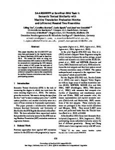
namely paragraphs, sentences, words and word senses [28]. The task had four subtasks: Paragraph–Sentence (compare a paragraph with a sentence), Sentence– Phrase (compare a sentence with a phrase), Phrase–Word (compare a phrase with a word) and Word–Sense (compare a word with a WordNet sense). The dataset for the task was derived from a wide variety of genres, including newswire, travel, scientific, review, idiomatic, slang, and search. Table 3 shows a few example pairs for the task. Each subtask used a training and testing dataset of 500 text pairs each. 2.2 Architecture of SemSim The SemSim system is composed of several modules designed to handle the computation of a similarity score among pieces of text in di↵erent languages and of di↵erent lengths. Figure 1 shows its high-level architecture, which has two main modules, one for computing the similarity of two words and another for two text sequences. The latter includes submodules for English, Spanish, and text sequences of di↵ering length. At the core of our system is the Semantic Word Similarity Model, which is based on a combination of latent semantic analysis and knowledge from WordNet (see Section 3). The model was created using a very large and balanced text corpus augmented with external dictionaries such as Wordnik and Urban Dictionary to improve handling of out-of-vocabulary tokens. The Semantic Text Similarity module manages the di↵erent inputs of the system, texts in English and Spanish and with varying length, and uses the semantic word similarity model to compute the similarity between the given pieces of text (see Section 4). It is supported by subsystems to handle the di↵erent STS tasks: – The English STS module is in charge of computing the similarity between English sentences (see Section 4.1). It preprocesses the text to adapt it to the word similarity model and align the terms extracted from the text to create

6

Abhay Kashyap et al.

Fig. 1 High-level architecture of the SemSim system with the main modules.

a term alignment score. Then, it uses di↵erent supervised and unsupervised models to compute the similarity score. – The Spanish STS module computes the similarity between Spanish sentences (see Section 4.2). It makes use of an external statistical machine translation [7] software (Google Translate) to translate the sentences to English. Then, it enriches the translations by considering the possible multiple translations of each word. Finally, it uses the English STS module to compute the similarity between the translated sentences and combine the results obtained. – The Cross-Level STS module is used to produce the similarity between text sequences of varying lengths, such as words, senses, and phrases (see Section 4.3). It combines the features obtained by the English STS module with features extracted from external dictionaries and Web search engines. In the following sections we detail the previous modules and in Section 5 we show the results obtained by SemSim at the di↵erent SemEval competitions. 3 Semantic Word Similarity Model Our word similarity model was originally developed for the Graph of Relations project [52] which maps informal queries with English words and phrases for an RDF linked data collection into a SPARQL query. For this, we wanted a similarity

A Robust Semantic Text Similarity System

7

metric in which only the semantics of a word is considered and not its lexical category. For example, the verb “marry” should be semantically similar to the noun “wife”. Another desiderata was that the metric should give highest scores and lowest scores in its range to similar and non-similar words, respectively. In this section, we describe how we constructed the model by combining latent semantic analysis (LSA) and WordNet knowledge and how we handled out-of-vocabulary words.

3.1 LSA Word Similarity LSA word similarity relies on the distributional hypothesis that the words occurring in similar contexts tend to have similar meanings [25]. Thus, evidence for word similarity can be computed from a statistical analysis of a large text corpus. A good overview of the techniques for building distributional semantic models is given in [32], which also discusses their parameters and evaluation. Corpus Selection and Processing. A very large and balanced text corpus is required to produce reliable word co-occurrence statistics. After experimenting with several corpus choices including Wikipedia, Project Gutenberg e-Books [26], ukWaC [5], Reuters News stories [46], and LDC Gigawords, we selected the Web corpus from the Stanford WebBase project [50]. We used the February 2007 crawl, which is one of the largest collections and contains 100 million web pages from more than 50,000 websites. The WebBase project did an excellent job in extracting textual content from HTML tags but still o↵ers abundant text duplications, truncated text, non-English text and strange characters. We processed the collection to remove undesired sections and produce high quality English paragraphs. Paragraph boundaries were detected using heuristic rules and only paragraphs with at least two hundred characters were retained. We eliminated non-English text by checking the first twenty words of a paragraph to see if they were valid English words. We used the percentage of punctuation characters in a paragraph as a simple check for typical text. Duplicate paragraphs were recognized using a hash table and eliminated. This process produced a three billion word corpus of good quality English, which is available at [20]. Word Co-Occurrence Generation. We performed part of speech (POS) tagging and lemmatization on the WebBase corpus using the Stanford POS tagger [51]. Word/term co-occurrences were counted in a moving window of a fixed size that scanned the entire corpus4 . We generated two co-occurrence models using window sizes ±1 and ±45 because we observed di↵erent natures of the models. ±1 window produces a context similar to the dependency context used in [34]. It provides a more precise context, but only works for comparing words within the same POS category. In contrast, a context window of ±4 words allows us to compute semantic similarity between words with di↵erent POS tags. 4 We used a stop-word list consisting of only the articles “a”, “an” and “the” to exclude words from the window. All remaining words were replaced by their POS-tagged lemmas. 5 Notice that ±4 includes all words up to ±4 and so it includes words at distances ±1, ±2, ±3, and ±4.

8

Abhay Kashyap et al.

A DT passenger NN plane NN has VBZ crashed VBN shortly RB after IN taking VBG o↵ RP from IN Kyrgyzstan NNP ’s POS capital NN , , Bishkek NNP , , killing VBG a DT large JJ number NN of IN those DT on IN board NN . . Fig. 2 An example of a POS-tagged sentence.

Our experience has led us to conclusion that the ±1 window does an e↵ective job of capturing relations, given a good-sized corpus. A ±1 window in our context often represents a syntax relation between open-class words. Although long distance relations can not be captured by this small window, this same relation can also appear as ±1 relation. For example, consider the sentence “Who did the daughter of President Clinton marry?”. The long distance relation “daughter marry” can appear in another sentence “The married daughter has never been able to see her parent again”. Therefore, statistically, a ±1 window can capture many of the relations the longer window can capture. While the relations captured by ±1 window can be wrong, the state-of-the-art statistical dependency parsers can produce errors, too. Our word co-occurrence models were based on a predefined vocabulary of about 22,000 common English words and noun phrases. The 22,000 common English words and noun phrases are based on the online English Dictionary 3ESL, which is part of the Project 12 Dicts6 . We manullay exclude proper nouns from the 3ESL because there are not many of them and they are all ranked at the top places since proper nouns start with an uppercase letter. WordNet is used to assign part of speech tags to the words in the vocabulary because statistical POS parsers can generate incorrect POS tags to words. We also added more than 2,000 verb phrases extracted from WordNet. The final dimensions of our word co-occurrence matrices are 29,000 ⇥ 29,000 when words are POS tagged. Our vocabulary includes only open-class words (i.e., nouns, verbs, adjectives and adverbs). There are no proper nouns (as identified by [51]) in the vocabulary with the only exception of an exploit list of country names. We use a small example sentence, “A passenger plane has crashed shortly after taking o↵ from Kyrgyzstan’s capital, Bishkek, killing a large number of those on board.”, to illustrate how we generate the word co-occurrence models. The corresponding POS tagging result from the Stanford POS tagger is shown in Figure 2. Since we only consider open-class words, our vocabulary for this small example will only contains 10 POS-tagged words in alphabetical order: board NN, capital NN, crash VB, kill VB, large JJ, number NN, passenger NN, plane NN, shortly RB and take VB. The resulting co-occurrence counts for the context windows of size ±1 and ±4 are shown in Table 4 and Table 5, respectively. Stop words are ignored and do not occupy a place in the context window. For example, in Table 4 there is one co-occurrence count between “kill VB” and “large JJ” in the ±1 context window although there is an article “a DT” between them. Other close-class words still occupy places in the context window although we do not need to count co-occurrences when they are involved since they are not in our vocabulary. For example, the co-occurrences count is zero between “shortly RB” and “take VB” in Table 4 since they are separated by “after IN” that is not a stop word. The reasons we only choose three articles as stop words are (1) they have high frequency in text; (2) they have few meanings; (3) we want 6

http://wordlist.aspell.net/12dicts-readme

A Robust Semantic Text Similarity System

9

Table 4 The word co-occurrence counts using ±1 context window for the sentence in Figure 2. word POS board NN capital NN crash VB kill VB large JJ number NN passenger NN plane NN shortly RB take VB

# 1 2 3 4 5 6 7 8 9 10

1 0 0 0 0 0 0 0 0 0 0

2 0 0 0 0 0 0 0 0 0 0

3 0 0 0 0 0 0 0 0 1 0

4 0 0 0 0 1 0 0 0 0 0

5 0 0 0 1 0 1 0 0 0 0

6 0 0 0 0 1 0 0 0 0 0

7 0 0 0 0 0 0 0 1 0 0

8 0 0 0 0 0 0 1 0 0 0

9 0 0 1 0 0 0 0 0 0 0

10 0 0 0 0 0 0 0 0 0 0

Table 5 The word co-occurrence counts using ±4 context window for the sentence in Figure 2. word POS board NN capital NN crash VB kill VB large JJ number NN passenger NN plane NN shortly RB take VB

# 1 2 3 4 5 6 7 8 9 10

1 0 0 0 0 0 1 0 0 0 0

2 0 0 0 1 0 0 0 0 0 0

3 0 0 0 0 0 0 1 1 1 1

4 0 1 0 0 1 1 0 0 0 0

5 0 0 0 1 0 1 0 0 0 0

6 1 0 0 1 1 0 0 0 0 0

7 0 0 1 0 0 0 0 1 1 0

8 0 0 1 0 0 0 1 0 1 0

9 0 0 1 0 0 0 1 1 0 1

10 0 0 1 0 0 0 0 0 1 0

to keep a small number of stop words for ±1 window since close-class words can often isolate unrelated open-class words; and (4) we want to capture the relation in the pattern “verb + the (a, an) + noun” that frequently appear in text for ±1 window, e.g., “know the person”. SVD Transformation. Singular value decomposition (SVD) has been found to be e↵ective in improving word similarity measures [31]. SVD is typically applied to a word by document matrix, yielding the familiar LSA technique. In our case we apply it to our word by context word matrix. In literature, this variation of LSA is sometimes called HAL (Hyperspace Analog to Language) [9]. Before performing SVD, we transform the raw word co-occurrence count fij to its log frequency log(fij + 1). We select the 300 largest singular values and reduce the 29K word vectors to 300 dimensions. The LSA similarity between two words is defined as the cosine similarity of their corresponding word vectors after the SVD transformation. LSA Similarity Examples. Table 6 shows ten examples obtained using LSA similarity. Examples 1 to 6 show that the metric is good at di↵erentiating similar from non-similar word pairs. Examples 7 and 8 show that the ±4 model can detect semantically similar words even with di↵erent POS while the ±1 model yields much worse performance. Examples 9 and 10 show that highly related but not substitutable words can also have a strong similarity, but the ±1 model has a better performance in discriminating them. We call the ±1 model concept similarity and the ±4 model relation similarity, respectively, since the ±1 model performs best

10

Abhay Kashyap et al.

Table 6 Ten examples from the LSA similarity model. # 1 2 3 4 5 6 7 8 9 10

Word Pair doctor NN, physician NN car NN, vehicle NN person NN, car NN car NN, country NN person NN, country NN child NN, marry VB wife NN, marry VB author NN, write VB doctor NN, hospital NN car NN, driver NN

±4 model 0.775 0.748 0.038 0.000 0.031 0.098 0.548 0.364 0.473 0.497

±1 model 0.726 0.802 0.024 0.016 0.069 0.000 0.274 0.128 0.347 0.281

on nouns and the ±4 model on relational phrases, regardless of their structure (e.g., “married to” and “is the wife of”). 3.2 Evaluation TOEFL Synonym Evaluation. We evaluated the ±1 and ±4 models on the wellknown 80 TOEFL synonym test questions. The ±1 and ±4 models correctly answered 73 and 76 questions, respectively. One question was not answerable because the question word, “halfheartedly”, is not in our vocabulary. If we exclude this question, ±1 achieves an accuracy of 92.4% and ±4 achieves 96.2%. It is worth mentioning that this outstanding performance is obtained without testing on the TOEFL synonym questions beforehand. According to ACL web page on state-of-the-art performance to TOEFL Synonym Questions,7 our result is second-to-best among all corpus-based approaches. The best performance was achieved by Bullinaria and Levy with a perfect accuracy but it was the result of directly tuning their model on the 80 questions. It is interesting that our models can perform so well, especially when our approach is much simpler than Bullinaria and Levy’s approach [8] or Rapp’s approach [44]. There are several di↵errences between our system and exiting approaches. First, we used a three-billion word corpus with high quality, which is larger than corpora used by Bullinaria and Levy (two-billion) or Rapp (100 million). Second, we performed POS tagging and lemmatization on the corpus. Third, our vocabulary includes only open-class or content words. WordSimilarity-353 Evaluation. WordSim353 is another dataset that is often used to evaluate word similarity measures [17]. It contains 353 word pairs, each of which is scored by 13 to 16 human subjects on a scale from 0 to 10. However, due to the limited size of the vocabulary that we used, some words in the WordSim353 dataset (e.g., “Arafat”) are outside of our vocabulary. Therefore, we chose to use a subset of WordSimilarity353 that had been used to evaluate a state-of-the-art word similarity measure PMImax [23] because both share the same 22,000 common English words as their vocabulary. This subset contains 289 word pairs. The evaluation result, including both the Pearson correlation and Spearman rank correlation 7

http://goo.gl/VtiObt

A Robust Semantic Text Similarity System

11

Table 7 Evaluating our LSA ±4 model on 289 pairs in WordSim353 dataset and comparing the results with the state-of-the-art word similarity measure PMImax [23]. PMImax LSA ±4 model

Pearson 0.625 0.642

Spearman 0.666 0.727

Table 8 Comparison of our LSA models to the Word2Vec model [41] on the 80 TOEFL synonym questions. Correctly Answered Accuracy Out-Of-Vocabulary Words

±1 model 73 92.4% halfheartedly

±4 model 76 96.2% halfheartedly

Word2Vec 67 84.8% tranquillity

coefficients, is shown in Table 7. Since WordSim353 is a dataset more suitable for evaluating semantic relatedness than semantic similarity, we only evaluate the ±4 model on it. The LSA ±4 model performed better than PMImax in both Pearson and Spearman correlation. If the 289 pairs could be thought as a representative sample of the 353 pairs and if we could thereby compare our result with the state-of-the-art evaluations on WordSimilarity-353 [1], the Pearson correlation of 0.642 produced by our model is ranked as the second to best among all state-of-the-art approaches. Comparison with Word2Vec. For the final evaluation, we also compared our LSA models to the Word2Vec [41] word embedding model on the TOEFL synonym questions. We used the pre-trained model also published by Mikolov et al. [41], which was trained on a collection of more than 100 billion words from Google News. The model contains 300-dimensional vectors, which has the same dimension as our models. One question word “tranquillity” is not in the pre-trained model’s vocabulary8 . Therefore, both sides have one question not answerable. The results of both systems are shown in Table 8. Our LSA models’ performance is significantly better than the Word2Vec model, at a 95% confidence level using the Binomial Exact Test. 3.3 Combining with WordNet Knowledge Statistical word similarity measures have limitations. Related words can have similarity scores only as high as their context overlap, as illustrated by “doctor” and “hospital” in Table 6. Also, word similarity is typically low for synonyms having many word senses since information about di↵erent senses are mixed together [23]. We can reduce the above issues by using additional information from WordNet. Boosting LSA similarity using WordNet. We increase the similarity between two words if any relation in the following eight categories hold: 1. They are in the same WordNet synset. 2. One word is the direct hypernym of the other. 3. One word is the two-link indirect hypernym of the other. 8

The spelling tranquillity dominated tranquility prior to 1980, but is now much less common.

12

Abhay Kashyap et al.

4. 5. 6. 7.

One adjective has a direct similar to relation with the other. One adjective has a two-link indirect similar to relation with the other. One word is a derivationally related form of the other. One word is the head of the gloss of the other or its direct hypernym or one of its direct hyponyms. 8. One word appears frequently in the glosses of the other and its direct hypernym. Notice that categories 1-6 are based on linguistic properties whereas categories 7-8 are more heuristic. We use the algorithm described in [12] to find a word gloss header.9 We define a word’s “significant senses” to deal with the problem of WordNet trivial senses. The word “year”, for example, has a sense “a body of students who graduate together” which makes it a synonym of the word “class”. This causes problems because this is not the most significant sense of the word “year”. A sense is significant if any of the following conditions are met: (i) it is the first sense; (ii) its WordNet frequency count is at least five; or (iii) its word form appears first in its synset’s word form list and it has a WordNet sense number less than eight. We require a minimum LSA similarity of 0.1 between the two words to filter out noisy data when extracting relations in the eight WordNet categories because some relations in the categories are not semantically similar. One is because our heuristic definition of ”significant sense” sometimes can include trivial sense of a word, therefore, noise. The second reason is that the derivational form of a word is not necessarily semantically similar to the word. The third reason is that the category 7 and 8 can produce incorrect results sometimes. We adopt the concept of path distance from [33] and assign path distance of zero to the category 1, path distance of one to the categories 2, 4, and 6, and path distance of two to categories 3, 5, 7, and 8. Categories 1-6 follow the definition in Li et al. but 7 and 8 are actually not related to path distance. However, in order to have a uniform equation to compute the score, we assume that these two categories can be boosted by a score equivalent to path length of 2, which is longest path distance in our eight categories. The new similarity between words x and y is computed by combining the LSA similarity and WordNet relations as shown in the following equation, sim (x, y) = min(1, simLSA (x, y) + 0.5e

↵D(x,y)

)

(1) ↵D(x,y)

where D(x, y) is the minimal path distance between x and y. Using e to transform simple shortest path length has been demonstrated to be very e↵ective by [33]. The parameter ↵ is set to 0.25, following their experimental results. Dealing with words of many senses. For a word w with many WordNet senses (currently ten or more), we use its synonyms with fewer senses (at most one third of that of w) as its substitutions in computing similarity with another word. Let Sx and Sy be the set of all such substitutions of the words x and y respectively. The new similarity is obtained using Equation 2. sim(x, y) = max(

max

sim (sx , y),

max

sim (x, sy ))

sx 2Sx [{x}

sy 2Sy [{y}

(2)

9 For example, the gloss of the first sense of “doctor” in WordNet is “a licensed medical practitioner”. The gloss head of “doctor” is therefore “practitioner”.

A Robust Semantic Text Similarity System

13

Table 9 Fraction of OOV words generated by Stanford POS tagger for a sample of 500 sentences per dataset. dataset MSRvid MSRpar SMT headlines OnWn

Noun 0.09 0.39 0.18 0.40 0.08

Adjective 0.27 0.37 0.19 0.44 0.10

Verb 0.04 0.01 0.03 0.02 0.01

Adverb 0.00 0.03 0.05 0.00 0.1

Finally, notice that some of the design choices in this section were made by intuition, observations, and a small number of sampled and manually checked experiments. Therefore some of the choices/parameters have a heuristic nature and may be suboptimal. The reason why we do so is because many parameters or choices in defining eight categories, “significant senses”, and similarity functions are intertwined. Due to the number of them, justifying every design choice requires many detailed experiments, which we cannot o↵er in this paper. The LSA+WordNet model was originally developed for Graph of Relation project or a schema-agnostic graph query system, as we pointed earlier in the paper. The advantage of LSA+WordNet model with these intuitive and pragmatic design choices over the pure LSA model has been demonstrated in the experiments on the graph query system [19]. An online demonstration of a similar model developed for the GOR project is available [53]. 3.4 Out-of-Vocabulary Words Our word similarity model is restricted by the size of its predefined vocabulary (set of (token, part of speech) tuples). Any word absent from this set is called an outof-vocabulary (OOV) word. For these, we can only rely on their lexical features like character unigrams, bigrams, etc. While the vocabulary is large enough to handle most of the commonly used words, for some domains OOV words can become a significant set. Table 9 shows the fraction of OOV words in a random sample of 500 sentences from the STS datasets when Stanford POS tagger was used. Table 10 gives some example OOV words. The most common type of OOV words are names (proper nouns) and their adjective forms. For example, the noun “Palestine” and its adjective form “Palestinian”. This is apparent from Table 9 where some datasets have high OOV nouns and adjectives due to the nature of their domain. For instance, MSRpar and headlines are derived from newswire and hence contain a large number of names of people, places, and organizations. Other OOV words include lexical variants (“summarise” vs “summarize”), incorrectly spelled words (“nterprise”), hyphenated words (multi-words), rare morphological forms, numbers, and time expressions. Since our vocabulary is actually a set of (token, part of speech) tuples, incorrect POS tagging also contributes to OOV words. Since OOV words do not have a representation in our word similarity model, we cannot compare them with any other word. One approach to alleviate this is to include popular classes of OOV words like names into our vocabulary. For highly focused domains like newswire or cybersecurity, this would be a reasonable

14

Abhay Kashyap et al.

Table 10 Examples of OOV words. POS Noun Adjective Verb Adverb

example OOV words gadhafi, spain, jihad, nterprise, jerry, biotechnology, health-care six-day, 20-member, palestinian, islamic, coptic, yemeni self-immolate, unseal, apologise, pontificate, summarise, plough faster, domestically, minutely, shrilly, thirdly, amorously

and useful approach. For instance, it would be useful to know that “Mozilla Firefox” is more similar to “Google Chrome” than “Adobe Photoshop”. However, for generic models, this would vastly increase the vocabulary size and would require large amounts of high quality training data. Also, in many cases, disambiguating named entities would be better than computing distributional similarity scores. For instance, while “Barack Obama” is somewhat similar to “Joe Biden” in that they both are politicians and democrats, in many cases it would be unacceptable to have them as substitutable words. Another approach is to handle these OOV terms separately by using a di↵erent representation and similarity function. Lexical OOV Word Similarity. We built a simple wrapper to handle OOV words like proper nouns, numbers and pronouns. We handle pronouns heuristically and check for string equivalence for numbers. For any other open class OOV word, we use simple character bigram representations. For example, the name “Barack” would be represented by the set of bigrams {‘ba’,‘ar’,‘ra’,‘ac’,‘ck’}. To compare a pair of words, we compute the Jaccard coefficient of their bigrams and then threshold the value to disambiguate the word pair.10 Semantic OOV Word Similarity. Lexical features work only for word disambiguation and make little sense when computing semantic similarity. While many OOV words come from proper nouns, for which disambiguation works well, languages continue to grow and add new words into their vocabulary. To simply use lexical features for OOV words would restrict the model’s ability to adapt to a growing language. For example, the word “google” has become synonymous with “search” and is often used as a verb. Also, as usage of social media and micro-blogging grows, new slang, informal words, abbreviations come into existence and become a part of common discourse. As these words are relatively new, including them in our distributional word similarity model might yield poor results, since they lack sufficient training data. To address this, we instead represent them by their dictionary features like definitions, usage examples, or synonyms retrieved from external dictionaries. Given this representation, we can then compute the similarity as the sentence similarity of their definitions [24, 29]. To retrieve reliable definitions, we need good sources of dictionaries with vast vocabulary and accurate definitions. We describe two dictionary resources that we used for our system. Wordnik [13] is an online dictionary and thesaurus resource that includes several dictionaries like the American Heritage dictionary, WordNet, and Wikitionary. It exposes a REST API to query their dictionary, although the daily usage limits 10 Our current system uses a threshold value of 0.8, which we observed to produce good results.

A Robust Semantic Text Similarity System

15

for the API adds a bottleneck to our system. Wordnik has a large set of unique words and their corresponding definitions for di↵erent senses, examples, synonyms, and related words. For our system, we use the top definition retrieved from the American Heritage dictionary and Wikitionary as context for an OOV word. We take the average of the sentence similarity scores between these two dictionaries and use it as our OOV word similarity score. Usually the most popular sense for a word is Wordnik’s first definition. In some cases, the popular sense was di↵erent between the American Heritage Dictionary and Wikitionary which added noise. Even with its vast vocabulary, several slang words and phrases were found to be absent in Wordnik. For this, we used content from the Urban Dictionary.

Urban Dictionary [54] is a crowd-sourced dictionary source that has a large collection of words and definitions added by users. This makes it a very valuable resource for contemporary slang words and phrases. Existing definitions are also subject to voting by the users. While this helps accurate definitions achieve a higher rank, popularity does not necessarily imply accuracy. We experimented with Urban Dictionary to retrieve word definitions for the Word2Sense subtask as described in Section 4.3.2. Due to the crowd-sourced nature of the resource, it is inherently noisy with sometimes verbose or inaccurate definitions. For instance, the top definition of the word “Programmer” is “An organism capable of converting ca↵eine into code” whereas the more useful definition “An individual skilled at writing software code” is ranked fourth.

4 Semantic Textual Similarity In this section, we describe the various algorithms developed for the *SEM 2013 and SemEval-2014 tasks on Semantic Textual Similarity.

4.1 English STS We developed two systems for the English STS task, which are based on the word similarity model explained in Section 3. The first system, PairingWords, uses a simple term alignment algorithm. The second system combines these scores with additional features for the given training data to train supervised models. We apply two di↵erent approaches to these supervised systems: an approach that uses generic models trained on all features and data (Galactus/Hulk ) and an approach that uses specialized models trained on domain specific features and data (Saiyan/SuperSaiyan).

Preprocessing. We initially process the text by performing tokenization, lemmatization and part of speech tagging, as required by our word similarity model. We use open-source tools from Stanford coreNLP [16] and NLTK [6] for these tasks. Abbreviations are expanded by using a complied list of commonly used abbreviations for countries, North American states, measurement units, etc.

16

Abhay Kashyap et al.

Term Alignment. Given two text sequences, we first represent them as two sets of relevant keywords, S1 and S2 . Then, for a given term t 2 S1 , we find its counterpart in the set S2 using the function g1 as defined by g1 (t) = argmax sim(t, t0 )

t 2 S1

t0 2S2

(3)

where sim(t, t0 ) is the semantic word similarity between terms t and t0 . Similarly, we define the alignment function g2 for the other direction as: g2 (t) = argmax sim(t, t0 )

t 2 S2

t0 2S1

(4)

g1 (t) and g2 (t) are not injective functions so their mappings can be many-toone. This property is useful in measuring STS similarity because two sentences are often not exact paraphrases of one another. Moreover, it is often necessary to align multiple terms in one sentence to a single term in the other sentence, such as when dealing with repetitions and anaphora, for example, mapping “people writing books” to “writers”. Term Weights. Words are not created equal and vary in terms of the information they convey. For example, the term “cardiologist” carries more information than the term “doctor”, even though they are similar. We can model the information content of a word as a function of how often it is used. For example, the word “doctor” is likely to have a larger frequency of usage when compared to “cardiologist” owing to its generic nature. The information content of a word w is defined as ! P 0 w0 ✏ C f req(w ) (5) ic(w) = ln f req(w) where C is the set of words in the corpus and f req(w) is the frequency of the word w in the corpus. For words absent in the corpus, we use average weight instead of maximum weight. It is a safer choice given that OOV words also include misspelled words or lexical variants. Term Alignment Score. We compute a term alignment score between any two text sequences as

T = mean

P

t2S1

ic(t) ⇤ sim(t, g1 (t)) P , t2S1 |ic(t)|

P

t2S2

ic(t) ⇤ sim(t, g2 (t)) P t2S2 |ic(t)|

!

(6)

where S1 and S2 are the sets of relevant key words extracted from their corresponding text, t represents a term, ic(t) represents its information content and g1 (t) or g2 (t) represents its aligned counterpart. The mean function can be the arithmetic or the harmonic mean.

A Robust Semantic Text Similarity System

17

4.1.1 PairingWords: Align and Penalize We hypothesize that STS similarity between two text sequences can be computed using ST S = T P 0 P 00 (7) where T is the term alignment score, P 0 is the penalty for bad alignments, and P 00 is the penalty for syntactic contradictions led by the alignments. However P 00 had not been fully implemented and is not used in our STS systems. We show it here just for completeness. We compute T from Equation 6 where the mean function represents the arithmetic mean. The similarity function sim0 (t, t0 ) is a simple lexical OOV word similarity back-o↵ (see Section 3.4) over sim(x, y) in Equation 2 that uses the relation similarity. We currently treat two kinds of alignments as “bad”, as described in Equation 8. The similarity threshold ✓ in defining Ai should be set to a low score, such as 0.05. For the set Bi , we have an additional restriction that neither of the sentences has the form of a negation. In defining Bi , we used a collection of antonyms extracted from WordNet [43]. Antonym pairs are a special case of disjoint sets. The terms “piano” and “violin” are also disjoint but they are not antonyms. In order to broaden the set Bi we will need to develop a model that can determine when two terms belong to disjoint sets. Ai = ht, gi (t)i |t 2 Si ^ sim0 (t, gi (t)) < ✓

Bi = {ht, gi (t)i |t 2 Si ^ t is an antonym of gi (t)} 0

i 2 {1, 2}

We show how we compute P in the following: P 0 ht,gi (t)i2Ai (sim (t, gi (t)) + wf (t) · wp (t)) A Pi = 2 · |Si | P 0 (sim (t, gi (t)) + 0.5) ht,g (t)i2B i i PiB = 2 · |Si | P 0 = P1A + P1B + P2A + P2B

(8)

(9)

wf (t) and wp (t) terms are two weighting functions on the term t. wf (t) inversely weights the log frequency of term t and wp (t) weights t by its part of speech tag, assigning 1.0 to verbs, nouns, pronouns and numbers, and 0.5 to terms with other POS tags. 4.1.2 Galactus/Hulk and Saiyan/Supersaiyan: Supervised systems The PairingWords system is completely unsupervised. To leverage the availability of training data, we combine the scores from PairingWords with additional features and learn supervised models using support vector regression (SVR). We used LIBSVM [10] to learn an epsilon SVR with a radial basis kernel and ran a grid search provided by [48] to find the optimal values for the parameters cost, gamma and epsilon. We developed two systems for the *SEM 2013 STS task, Galactus and Saiyan, which we used as a basis for the two systems developed for the SemEval-2014 STS task, Hulk and SuperSaiyan.

18

Abhay Kashyap et al.

Galactus and Saiyan: 2013 STS task. We used NLTK’s [6] default Penn Treebank based tagger to tokenize and POS tag the given text. We also used regular expressions to detect, extract, and normalize numbers, date, and time, and removed about 80 stopwords. Instead of representing the given text as a set of relevant keywords, we expanded this representation to include bigrams, trigrams, and skipbigrams, a special form of bigrams which allow for arbitrary distance between two tokens. Similarities between bigrams and trigrams were computed as the average of the similarities of its constituent terms. For example, for the bigrams “mouse ate” and “rat gobbled”, the similarity score is the average of the similarity scores between the words “mouse” and “rat” and the words “ate” and “gobbled”. Term weights for bigrams and trigrams were computed similarly. The aligning function is similar to Equation 3 but is an exclusive alignment that implies a term can only be paired with one term in the other sentence. This makes the alignment direction independent and a one-one mapping. We use refined versions of Google ngram frequencies [39], from [37] and [48], to get the information content of the words. The similarity score is computed by Equation 6 where the mean function represents the Harmonic mean. We used several word similarity functions in addition to our word similarity model. Our baseline similarity function was an exact string match which assigned a score of 1 if two tokens contained the same sequence of characters and 0 otherwise. We also used NLTK’s library to compute WordNet based similarity measures such as Path Distance Similarity, Wu-Palmer similarity [55], and Lin similarity [35]. For Lin similarity, the Semcor corpus was used for the information content of words. Our word similarity was used in concept, relation, and mixed mode (concept for nouns, relation otherwise). To handle OOV words, we used the lexical OOV word similarity as described in Section 3.4. We computed contrast features using three di↵erent lists of antonym pairs [43]. We used a large list containing 3.5 million antonym pairs, a list of about 22,000 antonym pairs from WordNet and a list of 50,000 pairs of words with their degree of contrast. The contrast score is computed using Equation 6 but the sim(t, t0 ) contains negative values to indicate contrast scores. We constructed 52 features from di↵erent combinations of similarity metrics, their parameters, ngram types (unigram, bigram, trigram and skip-bigram), and ngram weights (equal weight vs. information content) for all sentence pairs in the training data: – We used scores from the align-and-penalize approach directly as a feature. – Using exact string match over di↵erent ngram types and weights, we extracted eight features (4 ⇤ 2). We also developed four additional features (2 ⇤ 2) by including stopwords in bigrams and trigrams, motivated by the nature of MSRvid dataset. – We used the LSA-boosted similarity metric in three modes: concept similarity (for nouns), relation similarity (for verbs, adjectives and adverbs), and mixed mode. A total of 24 features were extracted (4 ⇤ 2 ⇤ 3). – For WordNet-based similarity measures, we used uniform weights for Path and Wu-Palmer similarity and used the information content of words (derived from the Semcor corpus) for Lin similarity. Skip bigrams were ignored and a total of nine features were produced (3 ⇤ 3).

A Robust Semantic Text Similarity System

19

Table 11 Fraction of OOV words generated by NLTK’s Penn Treebank POS tagger. dataset (#sentences) MSRpar (1500) SMT (1592) headlines (750) OnWN (1311)

Noun 0.47 0.26 0.43 0.24

Adjective 0.25 0.12 0.41 0.24

Verb 0.10 0.09 0.13 0.10

Adverb 0.13 0.10 0.27 0.23

– Contrast scores used three di↵erent lists of antonym pairs. A total of six features were extracted using di↵erent weight values (3 ⇤ 2). The Galactus system was trained on all of the STS 2012 data and used the full set of 52 features. The Saiyan system employed data-specific training and features. More specifically, the model for headlines was trained on 3000 sentence pairs from MSRvid and MSRpar, SMT used 1500 sentence pairs from SMT europarl and SMT news, while OnWN used only the 750 OnWN sentence pairs from last year. The FnWN scores were directly used from the Align-and-Penalize approach. None of the models for Saiyan used contrast features and the model for SMT also ignored similarity scores from exact string match metric. Hulk and SuperSaiyan: 2014 STS task. We made a number of changes for the 2014 tasks in an e↵ort to improve performance, including the following: – We looked at the percentage of OOV words generated by NLTK (Table 11) and Stanford coreNLP [16] (Table 9). Given the tagging inaccuracies by NLTK, we switched to Stanford coreNLP for the 2014 tasks. Considering the sensitivity of some domains to names, we extracted named entities from the text along with normalized numbers, date and time expressions. – While one-one alignment can reduce the number of bad alignments, it is not suitable when comparing texts of di↵erent lengths. This was true in the case of datasets like FrameNet-WordNet, which mapped small phrases with longer sentences. We thus decided to revert to the direction-dependent, many-one mapping used by the PairingWords system. – To address the high fraction of OOV words, the semantic OOV word similarity function as described in Section 3.4 was used. – The large number of features used in 2013 gave marginally better results in some isolated cases but also introduced noise and increased training time. The features were largely correlated since they were derivatives of the basic term alignment with minor changes. Consequently, we decided to use only the score from PairingWords and score computed using the semantic OOV word similarity. In addition to these changes Galactus was renamed Hulk and trained on a total of 3750 sentence pairs (1500 from MSRvid, 1500 from MSRpar and 750 from headlines). Datasets like SMT were excluded due to poor quality. Also, Saiyan was renamed SuperSaiyan. For OnWN, we used 1361 sentence pairs from previous OnWN dataset. For Images, we used 1500 sentence pairs from MSRvid dataset. The others lacked any domain specific training data so we used a generic training dataset comprising 5111 sentence pairs from MSRvid, MSRpar, headlines and OnWN datasets.

20

Abhay Kashyap et al.

Fig. 3 Our approach to compute the similarity between two Spanish sentences.

4.2 Spanish STS Adapting our English STS system to handle Spanish similarity would require to select a large and balanced Spanish text corpus and the use of a Spanish dictionary (such as the Multilingual Central Repository [18]). As a baseline for the SemEval-2014 Spanish subtask, we first considered translating the Spanish sentences to English and running the same systems explained for the English subtask (i.e., PairingWords and Hulk). The results obtained applying this approach to the provided training data were promising (with a correlation of 0.777). So, instead of adapting the systems to Spanish, we performed a preprocessing phase based on the translation of the Spanish sentences (with some improvements) for the competition (see Figure 3). Translating the sentences. To automatically translate sentences from Spanish to English we used the Google Translate API,11 a free, multilingual machine translation product by Google. It produces very accurate translations for European languages by using statistical machine translation [7], where the translations are generated on the basis of statistical models derived from bilingual text corpora. Google used as part of this corpora 200 billion words from United Nations documents that are typically published in all six official UN languages, including English and Spanish. In the experiments performed with the trial data, we manually evaluated the quality of the translations (one of the authors is a native Spanish speaker) and found the overall translations to be very accurate. Some statistical anomalies were noted that were due to incorrect translations because of the abundance of a specific 11

http://translate.google.com

A Robust Semantic Text Similarity System

21

word sense in the training set. On one hand, some homonym and polysemous words are wrongly translated which is a common problem of machine translation systems. For example, the Spanish sentence “Las costas o costa de un mar [...]” was translated to “Costs or the cost of a sea [...]”. The Spanish word costa has two di↵erent senses: “coast” (the shore of a sea or ocean) and “‘cost” (the property of having material worth). On the other hand, some words are translated preserving their semantics but with a slightly di↵erent meaning. For example, the Spanish sentence “Un coj´ın es una funda de tela [...]” was correctly translated to “A cushion is a fabric cover [...]”. However, the Spanish sentence “Una almohada es un coj´ın en forma rectangular [...]” was translated to “A pillow is a rectangular pad [...]”.12 Dealing with Statistical Anomalies. The aforementioned problem of statistical machine translation caused a slightly adverse e↵ect when computing the similarity of two English (translated from Spanish) sentences with the systems explained in Section 4.1. Therefore, we improved the direct translation approach by taking into account the di↵erent possible translations for each word in a Spanish sentence. For that, we used Google Translate API to access all possible translations for every word of the sentence along with a popularity value. For each Spanish sentence the system generates all its possible translations by combining the di↵erent possible translations of each word (in Figure 3 T S11 , T S12 ...T S1n are the possible translations for sentence SP ASent1). For example, Figure 4 shows three of the English sentences generated for a given Spanish sentence from the trial data. SPASent1: Las costas o costa de un mar, lago o extenso r´ıo es la tierra a lo largo del borde de estos. T S11 : Costs or the cost of a sea, lake or wide river is the land along the edge of these. T S12 : Coasts or the coast of a sea, lake or wide river is the land along the edge of these. T S13 : Coasts or the coast of a sea, lake or wide river is the land along the border of these. ... Fig. 4 Three of the English translations for the Spanish sentence SPASent1.

To control the combinatorial explosion of this step, we limited the maximum number of generated sentences for each Spanish sentence to 20 and only selected words with a popularity greater than 65. We arrived at the popularity threshold through experimentation on every sentence in the trial data set. After this filtering, our input for the “news” and “Wikipedia” tests (see Section 2.1) went from 480 and 324 pairs of sentences to 5756 and 1776 pairs, respectively. Computing the Similarity Score. The next step was to apply the English STS system to the set of alternative translation sentence pairs to obtain similarity scores (see T S11 vsT S21 ...T S1n vsT S2m in Figure 3). These were then combined to produce the final similarity score for the original Spanish sentences. An intuitive way 12 Notice that both Spanish sentences used the term coj´ ın that should be translated as cushion (the Spanish word for pad is almohadilla).

22

Abhay Kashyap et al.

Table 12 Fraction of OOV words in Phrase–Word and Word-Sense subtasks. dataset (1000 words)

OOV

examples

Phrase–Word

0.16

jingoistic, braless, bougie, skimp, neophyte, raptor

Word–Sense

0.25

swag, lol, cheapo, assload, cockblock, froofy

to combine the similarity scores would be to select the highest, as it would represent the possible translations with maximal similarity. However, it could happen that the pair with highest score have one or even two bad translations. We used this approach in our experiments with the trial data and increased the already high correlation from 0.777 to 0.785. We also tried another approach, computing the average score. Thus, given a pair of Spanish sentences, SP ASent1 and SP ASent2, and the set of possible translations generated by our system for each sentence, T rSent1 = {T S11 , . . . , T S1n } and T rSent2 = {T S21 , . . . , T S2m }, we compute the similarity between them by using the following formula:

SimSP A(SP ASent1, SP ASent2) =

n P m P

SimEN G(T S1i , T S2j )

i=1 j=1

n⇤m

where SimEN G(x, y) computes the similarity of two English sentences using our English STS systems. Using this approach and the trial data we increased the correlation up to 0.8. Thus, computing the average instead of selecting the best similarity score obtained a higher correlation for the trial data. Using a set of possible translations and averaging the similarity scores can help to reduce the e↵ect of wrong translations. We also speculate that the average behaved slightly better because it emulates the process followed to generate the gold standard, which was created by averaging the similarity score assigned to each pair of Spanish sentences by human assessors. 4.3 Cross-Level STS The SemEval-2014 task on Cross–Level Semantic Similarity presented a new set of challenges. For the Paragraph–Sentence and Sentence–Phrase subtask, we used the systems developed for the English STS with no modifications. However, the Phrase–Word and Word–Sense subtasks are specific to very short text sequences. If the constituent words are relatively rare in our model, there may not be sufficient discriminating features for accurate similarity computation. In the extreme case, if these words are not present at all in our vocabulary, the system would not be able to compute similarity scores. Table 12 shows the OOV fraction of the 1000 words from training and test datasets. While rare and OOV words can be tolerated in longer text sequences where the surrounding context would capture the relevant semantics, in tasks like these, performance is severely a↵ected by lack of context. 4.3.1 Phrase to Word As a baseline, we used the PairingWords system on the training set which yielded a very low correlation of 0.239. To improve performance, we used external resources to retrieve more contextual features for these words. Overall, there are

A Robust Semantic Text Similarity System

23

seven features: the baseline score from the PairingWords system, three dictionary based features, and three web search based features. Dictionary Features. In Section 3.4 we described the use of dictionary features as representation for OOV words. For this task, we extend it to all the words. To compare word and phrase, we retrieve a word’s definitions and examples from Wordnik and compare these with the phrase using our PairingWords system. The maximum score when definitions and examples are compared with the phrase constitutes two features in the algorithm. The intuition behind taking the maximum is that the word sense which is most similar to the phrase is selected. Following the 2014 task results, it was found that representing each phrase as a bag of words fared poorly for certain datasets, for example slang words and idioms. To address this, we added a third dictionary based feature based on the similarity of all Wordnik definitions of the phrase with all of the word’s definitions using our PairingWords system. This yielded a significant improvement over our results submitted in SemEval task as shown in Section 5. Web Search Features. Dictionary features come with their own set of issues, as described in Section 3.4. To overcome these shortcomings, we supplemented the system with Web search features. Since search engines provide a list of documents ranked by relevancy, an overlap between searches for the word, the phrase and a combination of the word and phrase, is evidence of similarity. This approach supplements our dictionary features by providing another way to recognize polysemous words and phrases, e.g., that ’java’ can refer to co↵ee, an island, a programming language, a Twitter handle, and many other things. It also addresses words and phrases that are at di↵erent levels of specificity. For example, ’object oriented programming language’ is a general concept and ’java object oriented programming language’ is more specific. A word or phrase alone lacks any context that could discriminate between meanings [42, 45]. Including additional words or phrases in a search query provides context that supports comparing words and phrases with di↵erent levels of specificity. Given the set A and a word or phrase pA where pA 2 A, a search on A will result in a set of relevant documents DA . Given the set B and a word or phrase pB where pB 2 B, if we search on B, we will receive a set of relevant documents for B given by DB . Both searches will return what the engine calculates as relevant given A or B. So if we search on a new set C which includes A and B, such that pA 2 C and pB 2 C then our new search result will be what the engine deems relevant, DC . If pA is similar to pB and neither are polysemous, then DA , DB and DC will overlap, shown in Figure 5(a). If either pA or pB is polysemous but not both, then there may only be overlap between either A and C or B and C, shown in Figure 5(b). If both pA and pB are polysemous, then the three document sets may not overlap, shown in Figure 5(c). In the case of a polysemous word or phrase, the overlapping likelihood is based on which meaning is considered most relevant by the search engine. For example, if pA is ’object oriented programming’ and pB is ’java’, there is a higher likelihood that ’object oriented programming’ + ’java’, pC , will overlap with either pA or pB if ’java’ as it relates to ’the programming language’ is most relevant. However, if ’java’ as it relates to ’co↵ee’ is most relevant then the likelihood of overlap is low. Specificity also a↵ects the likelihood of overlap. For example, even if the search engine returns a document set that is relevant to the intended meaning of ’java’

24

Abhay Kashyap et al.

or pB , the term is more specific than ’object oriented programming’ or pA and therefore less likely to overlap. However since the combination of ’object oriented programming’ + ’java’ or pC acts as a link between pA and pB , the overlap between A , C and B , C could allow us to infer similarity between A and B or similarity specifically between ’object oriented programming’ and ’java’.

(a)

(b)

(c)

(d) Fig. 5 (a) Overlap between A, B, and C; (b) overlap between ’A and C’ or ’B and C’; (c) no overlap between A, B and C; (d) overlap between ’A and C’ and ’B and C’.

We implemented this idea by comparing results of three search queries: the word, phrase, and the word and phrase together. We retrieved the top five results for each search using the Bing Search API13 and indexed the resulting document sets in Lucene [27] to obtain term frequencies for each search. For example, we created an index for the phrase ’spill the beans’, an index for the word ’confess’, and an index for ’spill the beans confess’. Using term frequency vectors for each we calculated the cosine similarity of the document sets. In addition, we also calculated the mean and minimum similarity among document sets. The similarity scores, the mean similarity, and minimum similarity were used as features, in addition to the dictionary features, for the SVM regression model. We evaluated how our performance improved given our di↵erent sets of features. Table 19 shows the cumulative e↵ect of adding these features. 4.3.2 Word to Sense For the Word to Sense evaluation, our approach is similar to that described in the previous section. However, we restrict ourselves to only dictionary features since using Web search as a feature is not easily applicable when dealing with word senses. We will use an example word author#n and a WordNet sense Dante#n#1 to explain the features extracted. We start by getting the word’s synonym set, Wi , from WordNet. For the word author#n, Wi comprises writer.n.01, generator.n.03 and author.v.01. We then retrieve their corresponding set of definitions, Di . The WordNet definition of writer.n.01, “writes (books or stories or articles or the like) 13

http://bing.com/developers/s/APIBasics.html

A Robust Semantic Text Similarity System

25

Table 13 Pearson’s correlation between the features and the annotated training data. feature F1 F2 F3 F4 F5 F6 F7 F8

correlation 0.391 0.375 0.339 0.363 0.436 0.410 0.436 0.413

professionally (for pay)” 2 Di . Finally, we access the WordNet definition of the sense, SD. In our example, for Dante#n#1, SD is “an Italian poet famous for writing the Divine Comedy that describes a journey through Hell and purgatory and paradise guided by Virgil and his idealized Beatrice (1265-1321)”. We use the PairingWords system to compute similarities and generate the following four features, where n is the number of word’s synonym set. – – – –

F1 F2 F3 F4

= max0i