Hierarchical Text Classification using Methods from Machine Learning

Hierarchical Text Classification using Methods from Machine Learning

Michael Granitzer

Hierarchical Text Classification using Methods from Machine Learning

Master’s Thesis at

Graz University of Technology submitted by

Michael Granitzer Institute of Theoretical Computer Science (IGI), Graz University of Technology A-8010 Graz, Austria

27th October 2003

c Copyright 2003 by Michael Granitzer

Advisor:

Univ.-Prof. DI Dr. Peter Auer

Hierarchische Textklassifikation mit Methoden des maschinellen Lernens

Diplomarbeit an der

Technischen Universit¨at Graz vorgelegt von

Michael Granitzer Institut f¨ur Grundlagen der Informationsverarbeitung (IGI), Technische Universit¨at Graz A-8010 Graz

27. Oktober 2003

c Copyright 2003, Granitzer Michael Diese Arbeit ist in englischer Sprache verfaßt.

Betreuer:

Univ.-Prof. DI Dr. Peter Auer

Abstract Due to the permantently growing amount of textual data, automatic methods for organizing the data are needed. Automatic text classification is one of this methods. It automatically assigns documents to a set of classes based on the textual content of the document. Normally, the set of classes is hierarchically structured but today’s classification approaches ignore hierarchical structures, thereby loosing valuable human knowledge. This thesis exploits the hierarchical organization of classes to improve accuracy and reduce computational complexity. Classification methods from machine learning, namely BoosTexter and the newly introduced CentroidBoosting algorithm, are used for learning hierarchies. In doing so, error propagation from higher level nodes and comparing decisions between independently trained leaf nodes are two problems which are considered in this thesis. Experiments are performed on the Reuters 21578, the Reuters Corpus Volume 1 and the Ohsumed data set, which are well known in literature. Rocchio and Support Vector Machines, which are state of the art algorithms in the field of text classification, serve as base line classifiers. Comparing algorithms is done by applying statistical significance tests. Results show that, depending on the structure of a hierarchy, accuracy improves and computational complexity decreases due to hierarchical classification. Also, the introduced model for comparing leaf nodes yields an increase in performance.

Kurzfassung Durch die starke Zunahme textueller Daten entsteht die Notwendigkeit automatische Methoden zur Datenorganisation einzusetzten. Automatische Textklassifikation ist eine dieser Techniken. Sie ordnet Textdokumente auf inhaltlicher Basis automatisch einer definierten Menge von Klassen zu. Die Klassen sind meist hierarchisch strukturiert, wobei die meisten heutigen Klassifikationsans¨atze diese Struktur ignorieren. Dadurch geht a priori Information verloren. Die vorliegende Arbeit besch¨aftigt sich mit dem Ausn¨utzen hierarchischer Strukturen zur Verbesserung von Genauigkeit und Zeitkomplexit¨at. BoosTexter und der hier neu vorgestellte CenroidBooster, Algorithmen aus dem Bereich des maschinellen Lernens, werden als hierarchische Klassifikationsmethoden eingesetzt. Die bei hierarchischer Klassifikation entstehenden Probleme der Fehlerfortpflanzung von hierarchisch h¨oheren Knoten und das Vergleichen von Entscheidungen aus unah¨angig trainierten Bl¨attern werden dabei ber¨ucksichtigt. Die Verfahren werden anhand bekannter Datens¨atze, dem Reuters-21578, Reuters Corpus Volume 1 und Ohsumed Datensatz analysiert. Dabei dienen Support Vector Maschinen und Rocchio, beides State of the Art Techniken als Vergleichsbasis. Die Vergleiche zwischen Ergebnissen erfolgen anhand statistischer Signifikanztests. Die Ergebnisse zeigen, daß abh¨angig von der hierarchischen Struktur, Genauigkeit und Zeitkomplexit¨at verbessert werden k¨onnen. Der Ansatz zum Vergleich von unabh¨angig trainierten Bl¨attern verbessert die Genauigkeit ebenfalls.

I hereby certify that the work presented in this thesis is my own and that work performed by others is appropriately cited. Ich versichere hiermit, diese Arbeit selbst a¨ ndig verfaßt, andere als die angegebenen Quellen und Hilfsmittel nicht benutzt und mich auch sonst keiner unerlaubten Hilfsmittel bedient zu haben.

Danksagung Ich m¨ochte an diesem Punkt meinen Eltern und Großeltern danken. Sie haben es mir erm¨oglicht, mein Studium und somit auch diese Arbeit in Angriff zu nehmen. Danke. Mein Dank gilt auch Professor Dr. Peter Auer, der mir die Gelegenheit gab, eine Diplomarbeit im Bereich des maschinellen Lernens zu verfassen und mir mit guten Ratschl¨age und Hinweisen zur Seite stand. Vielen herzliche Dank auch an meine Freundin Gisela D¨osinger, auf deren Hilfe ich immer z¨ahlen konnte und daß sie, sowie meine Arbeitskollegen Wolfgang Kienreich und Vedran Sabol, immer ein offenes Ohr f¨ur mich hatte. Die letzte Danksagung gilt meinem Arbeitgeber, dem Know-Center, fr das zu Verfgung stellen von technischen und zeitliche Ressourcen.

Der Weg ist das Ziel

Michael Granitzer Graz, Austria, Oktober 2003

i

Contents 1. Introduction and Problem Statement 1.1. Introduction . . . . . . . . . . . . . . . 1.1.1. Automatic Indexing . . . . . . 1.1.2. Document Organization . . . . 1.1.3. Text Filtering . . . . . . . . . . 1.1.4. Word Sense Disambiguation . . 1.2. Definitions and Notations . . . . . . . . 1.2.1. Notation . . . . . . . . . . . . 1.2.2. Definitions . . . . . . . . . . . 1.3. Problem Formulation . . . . . . . . . . 1.3.1. Text Classification . . . . . . . 1.3.2. Hierarchical Text Classification

. . . . . . . . . . .

. . . . . . . . . . .

. . . . . . . . . . .

. . . . . . . . . . .

. . . . . . . . . . .

. . . . . . . . . . .

. . . . . . . . . . .

. . . . . . . . . . .

. . . . . . . . . . .

. . . . . . . . . . .

. . . . . . . . . . .

. . . . . . . . . . .

. . . . . . . . . . .

. . . . . . . . . . .

. . . . . . . . . . .

. . . . . . . . . . .

2. State of Art Text Classification 2.1. Preprocessing-Document Indexing . . . . . . . . . . . . . . . . . . . 2.1.1. Term Extraction . . . . . . . . . . . . . . . . . . . . . . . . 2.1.2. Term Weighting . . . . . . . . . . . . . . . . . . . . . . . . . 2.1.3. Dimensionality Reduction . . . . . . . . . . . . . . . . . . . 2.1.3.1. Dimensionality Reduction by Term Selection . . . . 2.1.3.2. Dimensionality Reduction by Term Extraction . . . 2.2. Classification Methods . . . . . . . . . . . . . . . . . . . . . . . . . 2.2.1. Linear Classifiers . . . . . . . . . . . . . . . . . . . . . . . . 2.2.1.1. Support Vector Machines . . . . . . . . . . . . . . 2.2.1.2. Rocchio . . . . . . . . . . . . . . . . . . . . . . . 2.2.1.3. Multi-label Classification using Linear Classifiers . 2.2.2. Boosting . . . . . . . . . . . . . . . . . . . . . . . . . . . . 2.2.2.1. AdaBoost . . . . . . . . . . . . . . . . . . . . . . 2.2.2.2. Choice of Weak Learners and
 . . . . . . . . . . 2.2.2.3. Boosting applied to multi-label Problems . . . . . . 2.2.2.4. BoosTexter: Boosting applied to Text Classification 2.2.2.5. CentroidBoosting: An extension to BoosTexter . . . 2.2.3. Other Classification Methods . . . . . . . . . . . . . . . . . . 2.2.3.1. Probabilistic Classifiers . . . . . . . . . . . . . . . 2.2.3.2. Decision Tree Classifier . . . . . . . . . . . . . . . 2.2.3.3. Example Based Classifier . . . . . . . . . . . . . . 2.3. Performance Measures . . . . . . . . . . . . . . . . . . . . . . . . . 2.3.1. Precision and Recall . . . . . . . . . . . . . . . . . . . . . . 2.3.2. Other measurements . . . . . . . . . . . . . . . . . . . . . . 2.3.3. Combination of Precision and Recall . . . . . . . . . . . . . 2.3.4. Measuring Ranking performance . . . . . . . . . . . . . . . .

ii

. . . . . . . . . . . . . . . . . . . . . . . . . . . . . . . . . . . . .

. . . . . . . . . . . . . . . . . . . . . . . . . . . . . . . . . . . . .

. . . . . . . . . . . . . . . . . . . . . . . . . . . . . . . . . . . . .

. . . . . . . . . . . . . . . . . . . . . . . . . . . . . . . . . . . . .

. . . . . . . . . . . . . . . . . . . . . . . . . . . . . . . . . . . . .

. . . . . . . . . . . . . . . . . . . . . . . . . . . . . . . . . . . . .

. . . . . . . . . . . . . . . . . . . . . . . . . . . . . . . . . . . . .

. . . . . . . . . . .

1 1 2 2 2 2 2 2 3 3 3 4

. . . . . . . . . . . . . . . . . . . . . . . . . .

7 7 9 10 11 12 14 15 15 16 21 22 25 25 27 28 29 32 34 34 35 36 36 37 38 38 39

3. Hierarchical Classification

41

3.1. Basic Model . . . . . . . . . . . . . . . . . . . . . . . . . . . . . . . . . . . . . . .

41

3.2. Confidence of a decision . . . . . . . . . . . . . . . . . . . . . . . . . . . . . . . .

43

3.3. Learning the Classification Hypothesis . . . . . . . . . . . . . . . . . . . . . . . . .

46

3.4. Related Work . . . . . . . . . . . . . . . . . . . . . . . . . . . . . . . . . . . . . .

47

4. Experiments and Results

51

4.1. Parameters, Algorithms and Indexing Methods

. . . . . . . . . . . . . . . . . . . .

51

4.1.1. Boosting . . . . . . . . . . . . . . . . . . . . . . . . . . . . . . . . . . . .

51

4.1.2. Base Line Classifiers . . . . . . . . . . . . . . . . . . . . . . . . . . . . . .

52

4.1.2.1.

Rocchio . . . . . . . . . . . . . . . . . . . . . . . . . . . . . . .

52

4.1.2.2.

. . . . . . . . . . . . . . . . . . . . . . . . . . . . . .

52

4.1.3. Document Indexing . . . . . . . . . . . . . . . . . . . . . . . . . . . . . . .

52

4.2. Used Performance Measures . . . . . . . . . . . . . . . . . . . . . . . . . . . . . .

53

4.2.1. Classification Performance . . . . . . . . . . . . . . . . . . . . . . . . . . .

53

4.2.2. Ranking Performance . . . . . . . . . . . . . . . . . . . . . . . . . . . . . .

53

4.2.3. Comparing Experiments . . . . . . . . . . . . . . . . . . . . . . . . . . . .

54

4.3. Datasets . . . . . . . . . . . . . . . . . . . . . . . . . . . . . . . . . . . . . . . . .

56

4.3.1. Reuters-21578 . . . . . . . . . . . . . . . . . . . . . . . . . . . . . . . . .

56

4.3.2. Reuters Corpus Volume 1 . . . . . . . . . . . . . . . . . . . . . . . . . . .

57

4.3.3. Ohsumed . . . . . . . . . . . . . . . . . . . . . . . . . . . . . . . . . . . .

57

4.4. Results . . . . . . . . . . . . . . . . . . . . . . . . . . . . . . . . . . . . . . . . . .

58

4.4.1. Standard Data sets . . . . . . . . . . . . . . . . . . . . . . . . . . . . . . .

58

4.4.2. Flat vs. Hierarchical . . . . . . . . . . . . . . . . . . . . . . . . . . . . . .

59

4.4.3. Robust Training Set Selection . . . . . . . . . . . . . . . . . . . . . . . . .

62

4.4.4. Ranking Performance . . . . . . . . . . . . . . . . . . . . . . . . . . . . . .

64

4.4.5. Computation Time . . . . . . . . . . . . . . . . . . . . . . . . . . . . . . .

69

   

5. Conclusion and Open Questions

71

A. Stopwordlist

73

B. Data Sets

74

B.1. Reuters 21578 . . . . . . . . . . . . . . . . . . . . . . . . . . . . . . . . . . . . . .

74

B.2. Significance Test Results . . . . . . . . . . . . . . . . . . . . . . . . . . . . . . . .

75

B.3. Reuters Corpus Volume 1-Hierarchical Structure

. . . . . . . . . . . . . . . . . . .

84

B.4. OHSUMED . . . . . . . . . . . . . . . . . . . . . . . . . . . . . . . . . . . . . . .

85

iii

List of Figures

2.1. Document Classification Process . . . . . . . . . . . . . . . . . . . . . . . . . . . .

7

2.2. Document Indexing . . . . . . . . . . . . . . . . . . . . . . . . . . . . . . . . . . .

8

2.3. Linear Classifier . . . . . . . . . . . . . . . . . . . . . . . . . . . . . . . . . . . . .

16

2.4. Maximum Margin Linear Classifier . . . . . . . . . . . . . . . . . . . . . . . . . .

17

2.5. Maximum Margin Linear Classifier in the non Separable Case . . . . . . . . . . . .

19

2.6. Kernel Transformation . . . . . . . . . . . . . . . . . . . . . . . . . . . . . . . . .

20

2.7. 1 vs. rest Classification . . . . . . . . . . . . . . . . . . . . . . . . . . . . . . . . .

23

2.8. Pairwise Classification . . . . . . . . . . . . . . . . . . . . . . . . . . . . . . . . .

24

2.9. A example decision tree . . . . . . . . . . . . . . . . . . . . . . . . . . . . . . . . .

35

3.1. Definition of Decision Nodes in a Hierarchy . . . . . . . . . . . . . . . . . . . . . .

42

3.2. Classification Model in a Decision Node . . . . . . . . . . . . . . . . . . . . . . . .

43

3.3. Confidence of Independent Classifier . . . . . . . . . . . . . . . . . . . . . . . . . .

44

3.4. Sigmoid Functions with different steepness . . . . . . . . . . . . . . . . . . . . . .

45

3.5. Robust Training Set Selection

. . . . . . . . . . . . . . . . . . . . . . . . . . . . .

47

4.1. Sigmoid Distribution on the Ohsumed Data Set for BoosTexter.RV and SVM . . . .

66

4.2. Sigmoid Distribution on some Classes of the Ohsumed Data Set for BoosTexter.RV and SVM . . . . . . . . . . . . . . . . . . . . . . . . . . . . . . . . . . . . . . . .

67

4.3. Sigmoid Distribution on the Ohsumed Data Set for CentroidBooster with  adaption

68

iv

List of Tables

2.1. Term Selection Functions . . . . . . . . . . . . . . . . . . . . . . . . . . . . . . . .

13

2.2. Contingency Table . . . . . . . . . . . . . . . . . . . . . . . . . . . . . . . . . . .

37

3.1. Related Work in Hierarchical Text Classification . . . . . . . . . . . . . . . . . . . .

48

4.1. Results Reuters 21578 . . . . . . . . . . . . . . . . . . . . . . . . . . . . . . . . .

58

4.2. Results RCV 1 Hierarchical vs. Flat Classification . . . . . . . . . . . . . . . . . . .

59

4.3. Significance Tests RCV 1 Flat vs. Hierarchical

. . . . . . . . . . . . . . . . . . . .

60

4.4. Results Ohsumed Hierarchical vs. Flat Classification . . . . . . . . . . . . . . . . .

61

4.5. Significance Tests Ohsumed Flat vs. Hierarchical . . . . . . . . . . . . . . . . . . .

61

4.6. Results for Robust Training Set Selection on the RCV 1

. . . . . . . . . . . . . . .

63

4.7. Results for Robust Training Set Selection on the Ohsumed Dataset . . . . . . . . . .

63

4.8. Ranking Results “Reuters 19” . . . . . . . . . . . . . . . . . . . . . . . . . . . . .

65

4.9. Ranking Results for Ohsumed . . . . . . . . . . . . . . . . . . . . . . . . . . . . .

66

4.10. Ranking Results for RCV 1 . . . . . . . . . . . . . . . . . . . . . . . . . . . . . . .

69

4.11. Learning and Classification time for different data sets . . . . . . . . . . . . . . . .

69

B.1. Reuters 19 Data Set . . . . . . . . . . . . . . . . . . . . . . . . . . . . . . . . . . .

74

B.2. Significance Tests Ohsumed Hierarchical . . . . . . . . . . . . . . . . . . . . . . .

76

B.3. Significance Tests Ohsumed Flat . . . . . . . . . . . . . . . . . . . . . . . . . . . .

77

B.4. Significance Tests Ohsumed Flat vs. Hierarchical . . . . . . . . . . . . . . . . . . .

78

B.5. Significance Tests for Robust Training Set Selection on the Ohsumed Data Set . . . .

79

B.6. Significance Tests RCV 1 Hierarchical . . . . . . . . . . . . . . . . . . . . . . . . .

80

B.7. Significance Tests RCV 1 Flat . . . . . . . . . . . . . . . . . . . . . . . . . . . . .

81

B.8. Significance Tests RCV 1 Flat vs. Hierarchical

. . . . . . . . . . . . . . . . . . . .

82

B.9. Significance Tests for Robust Training Set Selection on the RCV 1 Data Set . . . . .

83

B.10. Classes, Training and Test Documents per Level of the RCV 1 Hierarchy . . . . . . .

84

B.11. Classes, Training and Test Documents per Level of the Ohsumed Hierarchy . . . . .

86

v

1. Introduction and Problem Statement This chapter introduces the need for text classification in today’s world and gives some examples of application areas. Problems of flat text classification compared to hierarchical text classification and how they may be solved by incorporating hierarchical information are outlined. Given this motivation, a general mathematical formulation on flat and hierarchical text classification, which is the problem formulation for this thesis, concludes the chapter.

1.1.

Introduction

One common problem in the information age is the vast amount of mostly unorganized information. Internet and corporate Intranets continue to increase and organization of information becomes an important task for assisting users or employees in storing and retrieving information. Tasks such as sorting emails or files into folder hierarchies, topic identification to support topic-specific processing operations, structured search and/or browsing have to be fulfilled by employees in their daily work. Also, available information on the Internet has to be categorized somehow. Web directories like for example Yahoo are build up by trained professionals who have to categorize new web sites into a given structure. Mostly this tasks are time consuming and sometimes frustrating processes if done manually. Categorizing new items manually has some drawbacks: 1. For special areas of interest, specialists knowing the area are needed for assigning new items (e.g. medical databases, juristic databases) to predefined categories. 2. Manually assigning new items is an error-prone task because the decision is based on the knowledge and motivation of an employee. 3. Decisions of two human experts may disagree (inter-indexing inconsistency) Therefore tools capable of automatically classifying documents into categories would be valuable for daily work and helpful for dealing with today’s information volume. A number of statistical classification and machine learning techniques like Bayesian Classifier, Support Vector Machines, rule learning algorithms, k-NN, relevance feedback, classifier ensembles, and neural networks have been applied to the task. Chapter 2 introduces traditional indexing and term selection methods as well as state of the art techniques for text classification. Multi-class classification using binary classifier and performance measurements are outlined. Issues of hierarchical text classification and the proposed model for this thesis are illustrated in chapter 3. Finally experiments and their results are presented in chapter 4 and the conclusion of this thesis is given in chapter 5. To give a motivation for text classification, this section concludes with application areas for automatic text classification.

1

1.1.1.

Automatic Indexing

Automatic Indexing deals with the task of describing the content of a document through assigning key words and/or key phrases. The key words and key phrases belong to a finite set of words called controlled vocabulary. Thus, automatic indexing can be viewed as a text classification task if each keyword is treated as separate class. Furthermore, if this vocabulary is a thematic hierarchical thesaurus this task can be viewed as hierarchical text classification.

1.1.2.

Document Organization

Document organization uses text classification techniques to assign documents to a predefined structure of classes. Assigning patents into categories or automatically assigning newspaper articles to predefined schemes like the IPTC Code (International Press and Telecommunication Code) are examples for document organization.

1.1.3.

Text Filtering

Document organization and indexing deal with the problem of sorting documents into predefined classes or structures. In text filtering there exist only two disjoint classes, relevant and irrelevant. Irrelevant documents are dropped and relevant documents are delivered to a specific destination. E-mail filters dropping “junk” mails and delivering “serious” mails are examples for text filtering systems.

1.1.4.

Word Sense Disambiguation

Word Sense Disambiguation tries to find the sense for an ambiguous word within a document by observing the context of this word (e.g. bank=river bank, financial bank). WSD plays an important role in machine translation and can be used to improve document indexing.

1.2.

Definitions and Notations

The following section introduces definitions and mathematical notations used in this thesis. For easier reading this section precedes the problem formulation.

1.2.1.

Notation

  Vectors are written lower case with an over lined arrow.  Sets are written bold, italic and upper case.  High dimensional (vector) spaces are written italic and upper case.  Matrices are written as German “Fraktur” characters and upper case.  Graphs are written calligraphic and upper case  "! Classes and Documents are written San Serif and upper case. $#&%('*),+.- returns / if the sign is positive, 01/ else. $234+ 5 returns / if the argument of 2 is true, 6 else. 78  + 9 denotes the inner product of two vectors

2

1.2.2.

Definitions

Since the implemented algorithms are used to learn hierarchies some preliminary definitions describing properties of such hierarchies and their relationship to textual documents and classes are given. Hierarchy (: ): A Hierarchy :=?@A- is defined as directed acyclic graph consisting of a set of nodes = and a set of ordered pairs called edges )CBEDFGBHI-KJL@NMPOQ= RS=UT . The direction of an edge )CBVDFGBH- is defined from the parent node BWD to the direct child node BXH , specified through the relational operator BWDEY7BH which is also called direct path from B1D to BH .

Z B\H with length ] is therefore an ordered set of nodes O^BA_VY`Ba1Ycbcbcb"GB\dfeg_VY A path BVD[Y$ B d TAMU= where each node is the parent node of the following node. In a hierarchy : with a path BVDSYZ B\H there exists no path BhHEYZ BiD since the hierarchy is acyclic. Additionally there exists exactly one node called root node Bkj of a graph : which has no parent.

Nodes which are no parent nodes are called leaf nodes. All nodes except leaf nodes and the root node are called inner nodes. Classes (  ): Each node B within a hierarchy : is assigned exactly to one class  : ). Each class  consists of a set of documents oJp .







l m =  (n

If not stated otherwise within this thesis, for each class  a classification hypothesis  lated. The form of q is given by the classification approach.



q 

J

is calcu-

Documents ( ! ): Documents of a hierarchy : contain the textual content and are assigned to one or more classes. The classes of a document are also called labels of a document rP; Ost_*bcbcb" T .

9

9

9

9yx z{x



_&v  awv bcbcb v where each In general each document is represented as term vector  ;Xu   9~} v i| dimension  represents the weight of a term obtained from preprocessing. Preprocessing and indexing methods are discussed in Section 2.1

1.3.

Problem Formulation

Since hierarchical text classification is an extension of flat text classification, the problem formulation for flat text classification is given first. Afterwards the problem definition is extended by including hierarchical structures (as defined in 1.2.2) which gives the problem formulation for this thesis.

1.3.1.

Text Classification

Text Classification is the task of finding an approximation for the unknown target function  € `R l Y Oc‚GƒhT , where  is a set of documents and l is a set of predefined} classes. Value  of the target function P€ „R l YoOc‚GƒhT is the decision to assign document ! JS to classes l J l  } J… and value ƒ is the decision not to assign document ! to classes  J l .  describes how  } J to classes  J l . The documents ought to be classified and in short assigns documents !  target function  is also called target concept and is element of a concept class  JA† .

‡ € `R l YˆOc‚GƒXT is called classifier or hypothesis and should The approximating function ? coincide with  as much as possible. This coincidence is called effectiveness and will be described in 2.3. A more detailed definition considering special constraints to the text classification tasks is given in [68].

3

For the application considered in this thesis the following assumptions for the above definition are made:





The target function  is described by a document corpus. A corpus is defined through the } J set of classes l , the set of documents  and the assignment of classes to documents ! ‰ } . No additional information for describing  is given. The document corpus is also called classification scheme. Documents ment.



are represented by a textual content which describes the semantics of a docu-



Categories l are symbolic labels for documents providing no additional information like for example meta data.



J  can be assigned to / bcbcb‹Š l Š categories (multi-label text classification). Documents ! Since this is a special case of binary text classification, where a document is assigned to a ‰ J *ŒVJ  l , algorithms and tasks for binary text classification are also category  l or not, considered.

}

For classifying documents automatically, the approximation

1.3.2.

‡

has to be constructed.

Hierarchical Text Classification

Supplementary to the definition of text classification a graph target function  , such that

:

is added for defining the unknown

 ‘  )Ž!’ } - ;   )Ž!  - ; …  } Y“Z  ’   }  J : b  

if

: is a hierarchical structure} defining relationships among classes. The assumption behind these constraints is, that  Y  defines a IS-A relationship among classes whereby  has a broader   } topic than  and the topic of a parent class  covers all topics ”•~–‹—™š ˜ –s› œ of its child classes.  Additionally topics from siblings differ from each other, but must not be exclusive to each other. Thus, topics from siblings may overlap 1 . The IS-A relationship is asymmetric (e.g. all dogs are animals, but not all animals are dogs) and transitive (e.g. all pines are evergreens and all evergreens are trees; therefore all pines are trees). The goal is, as before, to approximate the unknown target function by using a document corpus. Additionally the constraints defined by the hierarchy : have to be satisfied. Since classification methods depend on the given hierarchical structure including classes and assigned documents, the following basic properties can be distinguished:



Structure of the hierarchy: Given the above general definition of a hierarchy : , two basic cases can be distinguished. (i) A tree structure, where each class (except the root class) has exactly one parent class and (ii) a directed acyclic graph structure where a class can have more than one parent classes.

1

Which must be true for allowing multilabel classification

4



Classes containing documents: Another basic property is the level at which documents are assigned to classes within a hierarchy. Again two different cases can be distinguished. In the first case, documents are assigned only to leaf classes which is defined here as virtual hierarchy. In the second case a hierarchy may also have documents assigned to inner nodes. Note that the latter case can be extended to a virtual hierarchy by adding a virtual leaf node to each inner node. This virtual leaf node contains all documents of the inner node.



Assignment of documents As done in flat text classification, it can be distinguished between multi label and single label assignment of documents. Depending on the document assignment the classification approach may differ.

The model proposed here is a top-down approach to hierarchical text classification by using a directed acyclic graph. Additionally, multi label documents are allowed. A top down approach means that recursively, starting at the root node, at each inner node zero, one or more subtrees are selected by a local classifier. Documents are propagated into these subtrees till the correct class(es) is/are found. From a practical point of view, this thesis focuses on hierarchical text classification in document management systems. In such systems, text classification can be used in two ways:

 

Documents are automatically assigned to ][;

3 6 bcbcbsŠ l Š 5

classes

The users are provided with a ranked list of classes to which a document may belong to. The user can choose one of these classes to store the document. This task can be viewed as semi automatic classification. Additionally to the former way, a ranking mechanism between classes has to be applied.

Whereas the first task is similar to automatic indexing (where the hierarchy is a controlled vocabulary) the latter task may be viewed as a query, returning a ranked list of classes having the most suitable classes ranked top. Note that the latter task can be used to perform the former one, but not vice versa. This tasks can also be achieved by flat text classification methods, where the hierarchical relationship between classes is ignored when building the classifier. But in application areas like document organization and automatic indexing this may be a major loss of information. Document organization is mostly done in hierarchical structures, built up by humans using their knowledge on a specific domain. Using this knowledge might improve the classification. Viewed from the point of machine learning, having a lot of possible classifications usually leads to a complex concept class, thereby increasing learning time and decreasing generalization accuracy. Beneath this aspect, classification time in a flat model is linear with the amount of classes whereas a hierarchical model might allow only logarithmic classification time. This can be useful in settings where a large amount of documents has to be classified automatically into a big hierarchical structure. All these aspects point toward hierarchical text classification whereby two major problems arise in the machine learning setting: 1. Reducing error propagation 2. The validity of comparing classifications from different leaf nodes

5

Comparing results from different leaf nodes can not be achieved easily if the training of these leaf nodes is independent from each other. Leaf nodes dealing with an easier classification problem may produce higher confidence values2 than leaf nodes dealing with harder problems. So, if no additional mechanism regulates the comparison of leaf nodes, then results are hardly comparable. Furthermore, decisions for selecting the appropriate sub hierarchy have to be highly accurate. If wrong decisions are made early in the classification process 3 the error is propagated through the whole hierarchy leading to higher error rates than in a flat model. Solving these problems is a non-trivial task and the main focus of this thesis.

2 3

e.g. achieving a higher margin in the case of linear classifiers under the assumption of a weak heuristic for this sub hierarchy

6

2. State of Art Text Classification As stated in chapter 1.3 text classification is the task to approximate a unknown target function  through inductive construction of a classifier on a given data set. Afterward, new, unseen documents are assigned to classes using the approximate function ‡ . Within this thesis, the former task is referred to as “learning” and the latter task is called “classification”. As usual in classification tasks, learning and classification can be divided into the following two steps: 1. Preprocessing/Indexing is the mapping of document contents into a logical view (e.g. a vector representation of documents) which can be used by a classification algorithm. Text operations and statistical operations are used to extract important content from a document. The term logical view of a document was introduced in [4]. 2. Classification/Learning: based on the logical view of the document classification or learning takes place. It is important that for classification and learning the same preprocessing/indexing methods are used. Figure 2.1 illustrates the classification process. Each step above is further divided into several modules and algorithms. This chapter is organized as follows: an overview on algorithms and modules for document indexing is given in section 2.1. Various classification algorithms are introduced in section 2.2. Section 2.3 introduces performance measures for evaluating classifiers.

2.1.

Preprocessing-Document Indexing

As stated before, preprocessing is the step of mapping the textual content of a document into a logical view which can be processed by classification algorithms. A general approach in obtaining the logical view is to extract meaningful units (lexical semantics) of a text and rules for the combination of these units (lexical composition) with respect to language. The lexical composition is actually based on linguistic and morphological analysis and is a rather complex approach for preprocessing. Therefore, the problem of lexical composition is usually disregarded in text classification. One exception is given in [15] and [25], where Hidden Markov Models are used for finding the lexical composition of document sections. Documents D

Preprocessing

Logical View V

Classification

Classification C

Hierarchy H

Figure 2.1.: Document classification is divided into two steps: Preprocessing and classification.

7

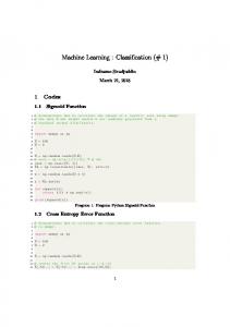
Document Indexing Term Extraction

Weightening

Lexical Analysis

Dimensionality Reduction

Stopword Removal

Stemming

Noun Groups

Structure Analysis

Figure 2.2.: Document indexing involves the main steps term extraction, term weighting and dimensionality reduction. By ignoring lexical composition the logical view of a document !ž can be obtained by extracting all meaningful units (terms) from all documents  and assigning weights to each term in a document reflecting the importance of a term within the document. More formally, each document is assigned 9 } ;Xu 8Ÿ_c&8a‹cbcbcb^&8’d | whereby each dimension represents a term from an ] -dimensional vector a term set   . The resulting ] -dimensional space is often referred to as Term Space of a document corpus. Each document is a point within this Term Space. So by ignoring lexical composition, preprocessing can be viewed as transforming character sequences into an ] -dimensional vector space. Obtaining the vector representation is called Document Indexing and involves two major steps: 1. Term Extraction: Techniques for defining meaningful terms of a document corpus (e.g. lexical analysis, stemming, word grouping etc.) 2. Term Weighting Techniques for defining the importance of a term within a document (e.g. Term Frequency, Term Frequency Inverse Document Frequency) Figure 2.2 shows the steps used for document indexing and their dependencies. Document Indexing yields to a high dimensional term space whereby only a few terms contain important information for the classification task. Beside the higher computational costs for classification and training, some algorithms tend to overfit in high dimensional spaces. Overfitting means that algorithms classify all examples of the training corpus rather perfect, but fail to approximate the unknown target concept  (see 2.1.3). This leads to poor effectiveness on new, unseen documents. Overfitting can be reduced by increasing the amount of training examples. It has been shown in [28] that about 50-100 training examples may be needed per term to avoid overfitting. For this reasons dimensionality reduction techniques should be applied. The rest of this section illustrates well known techniques for term selection/extraction (see 2.1.1), weighting algorithms (see 2.1.2) and the most important techniques for applying dimensionality reduction (see 2.1.3).

8

2.1.1.

Term Extraction

Term extraction, often referred to as feature extraction, is the process of breaking down the text of a document into smaller parts or terms. Term extraction results in a set of terms   which are used for the weighting and dimensionality reduction steps of preprocessing. In general the first step is a lexical analysis where non letter characters like sentence punctuation and styling information (e.g. HTML Tags) are removed. This reduces the document to a list of words separated by whitespace. Beneath the lexical analysis of a document, information about the document structure like sections, subsections, paragraphs etc. can be used to improve the classification performance, especially for long documents. Incorporating structural information of documents has been done in various studies ( see [39], [33] and [72]). Doing a document structure analysis may lead to a more complex representation of documents making the term space definition hard to accomplish (see [15]). Most experiments in this area have shown that performance over larger documents can be increased by extracting structures and subtopics from documents. Identifying terms by words of a document is often called set of words or bag of words approach, depending on whether weights are binary or not. Stopwords, which are topic neutral words such as articles or prepositions contain no valuable or critical information. These words can be safely removed, if the language of a document is known. Removing stopwords reduces the dimensionality of term space. On the other hand, as shown in [58], a sophisticated usage of stopwords (e.g. negation, prepositions) can increase classification performance. One problem in considering single words as terms is the semantic ambiguity (e.g. river bank, financial bank) which can be roughly categorized in:

 

Synonyms: A synonym is a word which means the same as another word (e.g. Movie ¡

Y

Film).

Homonym: A homonym refers to a word which can have two or more meanings (e.g. lie).

Since only the context of the word within a sentence or document can dissolve this ambiguity, sophisticated methods like morphological and linguistic analysis are needed to diminish this problem. In [23] morphological methods are compared to traditional indexing and weighting techniques. It was stated, that morphological methods slightly increase classification accuracy for the cost of higher computational preprocessing. Additionally, these methods have a higher impact on morphologically richer languages, like for example German, than simpler languages, like for example English. Also, text classification methods have been applied to this “Word Sense Disambiguity” problem (see [30]). Beside synonymous and homonymous words, different syntactical forms may describe the same word (e.g. go, went, walk, walking). Methods for extracting the syntactical meaning of a word are suffix stripping or stemming algorithms 1 . Stemming is the notation for reducing words to their word stems. Most words in the majority of Western languages can be “stemmed” by deleting (stripping) language dependent suffixes from the word (e.g. CONNECTED,CONNECTING ‘ CONNECT). On the other hand, stripping can lead to new ambiguities (e.g. RELATIVE,RELATIVITY) so that more sophisticated methods performing linguistic analysis may be useful. The performance of stripping and stemming algorithms depends strongly on the simplicity of the used language. For English a lot of stripping and stemming algorithms exist, the Porters Algorithm [55] being the most popular one. 1

Which are language dependent algorithms

9

Recently a German stemming algorithm [9] has been incorporated into the Lucene Jakarta project and is also freely available. Taking noun groups, which consist of more than one word as term, seems to capture more information. In a number of experiments single word terms were replaced by word grams 2 or phrases. As stated in [3],[19], [40] and [8] this did not give a significantly better performance. A language independent method for extracting terms is called character n-grams. This approach was first discussed by Shannon [69] and further extended by Suen [71]. A character n-gram is a sequence of n characters occurring in a word and can be obtained by simply moving a window of length n over a text (sliding one character at the time) and taking the actual content of a window as term. N-gram representation has the advantage of being language independent and of learning garbled messages. As stated in [24] stemming and stopword removal are superior for word-based systems but are not significantly better for an n-gram based system. The major drawback of n-grams is the amount of unique terms which can occur within a document corpus. Additionally, character ngrams in Information Retrieval (IR) systems yield to the incapability of replacing synonymous words within a query. In [45] it is stated, that the number of unique terms for 4-grams is around equal to the number of unique terms in a word based system. Experiments in [10] have shown that character ngrams are suitable for text classification tasks. Also, character n-grams have been sucessfully applied to clustering and visualizing search results (see [31]).

2.1.2.

Term Weighting

After extracting the term space from a document corpus the influence of each term within a document has to be determined. Therefore each term ¢ within a document is assigned a weight 8 leading to  9  }  8Ÿ_"&8abcbcb"&8’d the above described vector representation of a document. The most simple ;Xu | approach is to assign binary values as weights indicating the presence or absence of a term. A more general approach for weighting is counting the occurrences of terms within a document normalized HªHŽ«  › v­¬¯® ° by the amount of words within a document, the so called term frequency £¥¤(¦"§ ) ¢ œs"! Œ - ;©¨ ± . Thereby B is the number of terms in !KŒ and ²‹³³ ) ¢ œf"!´Œ - is the number of occurrences of term ¢ œ in ! Œ. The term frequency approach seems to be very intuitive, but has a major drawback. For example function words occur often within a document and they have a high frequency, but since these words occur in nearly all documents they carry no information about the semantics of a document. This circumstances correspond to the well known Zip-Mandelbrot law [42] which states, that the frequency of terms in texts is extremely uneven. Some terms occur very often, whereas as a rule of thumb, half of the terms occur only once. Similar to term frequencies, logarithmic frequencies as

£¥¤(¦"§ ) ¢ œf"!´Œ - ;…µ·¶ ¥% ) ´ / ¸$£¥¤(¦"§ ) ¢ œ("!¹Œ -&¨

may be taken, which is a more common measure in quantitative linguistics (see [23]). Again, logarithmic frequency suffers from the drawback, that function words may occur very often in the text. To overcome this drawback, weighting schemes are applied for transforming these frequencies into more meaningfull units. One standard approach is the inverse document frequency (idf) weighting function which has been introduced by [62]

Š …Š 8œ v P ; £¥¤(¦"§ ) ¢ œ("!¹Œ.-{º µ·¶ % Š Of!´Œ»J¼½Š œJ¾!¹ŒT¿Š ¢

and is know as Term Frequency Inverse Document Frequency (TFIDF) weighting scheme. Thereby £¥¤(¦"§ ) ¢ œ("! Œ - denotes the term frequency of term ¢ œ within document À ,  denotes the set of available 2

n-word grams are a sequence of n words consequently occurring in a document

10

documents and Of!tŒyJpÁŠ ¢ œXJÂ!¹Œ.T denotes the set of documents containing term ¢ œ . In other words a term is relevant for a document if it (i) occurs frequently within a document and (ii) discriminates between documents by occurring only in a few documents. For reducing the effects of large differences between frequencies of terms a logarithmic or square root function can be applied to the term frequency leading to

Š …Š 8œ v P ; £¥¤(¦^§ ) ¢ œ v  -{º µ·¶ % Š Of! Œ JS½Š œJ¾! Œ T¿Š ¨ ¢ or

Š …Š 8œ v  ; à £¥¤(¦"§ ) ¢ œ v  - º µ·¶ % Š Of!¹Œ»JS½Š œJ¾!¹Œ.T¿Š ¢ TFIDF weighting is the standard weighting scheme within text classification and information retrieval. Another markable weighting technique is the entropy weighting scheme which is calculated as

where

8œ v P ) œ v -ĺV) /t¸$¦c]g¢,¤s²Å™Æ ) ¢ œ(-& ; £¥¤(¦"§ ¨ ¢  x ÇEx È ²‹³w³ ) ¢ œf"!gžÊ- º % ²‹³³ / ¦c]g¢,¤s²Å™Æ ) ¢ œ(- ; %WŠ Š }wÉ _ µ·¶ µ·¶ ²‹³w³ ) ¢ œ¿²‹³³

) ¢ œ¿"!žª) ¢ œ¿Â-

is the entropy of term Ë . As stated in [20] the entropy weighting scheme yields better results than TFIDF or other ones. A comparison of different weighting schemes is given in [62] and [23]. Additionally, weighting approaches can be found in [11], [12] and in the AIR/X system [29]. After having determined the influence of a term by using frequency transformation and weighting, the length of terms has to be considered by normalizing documents to unique length. From a linguistic point of view normalizing is a non trivial task (see [43],[51]). A good approximation is to divide term frequencies by the total number of tokens in text which is equivalent to normalize the vector using the one norm: 8

8 œ ; Ì Ì 8 _

Since some classification algorithms (e.g. SVM’s) yield better error bounds by using other norms (e.g. euclidean), these norms are frequently used within text classification.

2.1.3.

Dimensionality Reduction

Document indexing by using the above methods leads to a high dimensional term space. The dimensionality depends on the number of documents in a corpus, for example the 20.000 documents of the Reuters 21578 data set (see section 4) have about 15.000 different terms. Two major problems arise having a that high dimensional term space: 1. Computational Complexity: Information retrieval systems using cosine measure can scale up to high dimensional term spaces. But the learning time of more sophisticated classification algorithms increases with growing dimensionality and the volume of document copora.

11

2. Overfitting: Most classifiers (except Support Vector Machines [35]) tend to overfit in high dimensional space, due to the lack of training examples. To deal with these problems, dimensionality reduction is performed keeping only terms with valuable information. Thus, the problem of identifying irrelevant terms has to be solved for obtaining a reduced term space ͏ΠÏÐÍ with Š ͒ЊFÑҊ Í Š . Two distinct views of dimensionality reduction can be given:



Local dimensionality reduction: For each class





Í Î  QŠ ͒Π Š(ÑÁŠ Í Š  , a set ’

is chosen for classification under



.

Global dimensionality reduction: a set

Í Î Q Š Í Î Š 1 u u ŠÍ Š

is chosen for the classification under all categories

l

Mostly, all common techniques can perform local and global dimensionality reduction. Therefore the techniques can be distinguished in another way:





by term selection: According to information or statistical theories a subset space Í .

Í Î

of terms is taken from the original

by term extraction terms in the new term space Í Î are obtained through a transformation of ͒Πmay be of a complete different type than in Í .

2.1.3.1.

Í Î ;UÓ ) Í - . The terms

Dimensionality Reduction by Term Selection

The first approach on dimensionality reduction by term selection is the so called filtering approach. Thereby measurements derived from information or statistical theory are used to filter irrelevant terms. Afterwards the classifier is trained on the reduced term space, independent of the used “filter function”. Another approach are so called wrapper techniques (see [48]) where term selection based on the used classification algorithm is proposed. Starting from an initial term space a new term space is generated by adding or removing terms. Afterwards the classifier is trained on the new term space and tested on a validation set. The term space yielding best results is taken as term space for the classification algorithm. Having the advantage of a term space tuned on the classifier, the computational cost of this approach is a huge drawback. Therefore, wrapper approaches will be ignored in the rest of this section. Document Frequency: A simple reduction function is based on the document frequency of a term ¢ œ . According to the Zipf-Mandelbrot law, the highest and lowest frequencies are discarded. Experiments indicate that a reduction of a factor 10 can be performed without loss of information.

12

Function DIA association factor Information gain

£ Ô) *Œ4 ¢ œ‹Õ ) ¢ œ¯gŒ ØFÙ ) ¢ œ¯gŒ. Ø ) ¢ œf*Œ.a æ ) ¢ œ¯gŒ B ÙWè ) ¢ œ¯ Œ ëE ) ¢ œ( Œ îWë ) ¢ œf*Œ Ù1 ) ¢ œf*Œ.-

Mathematical form

Ö ¤ 3·)ÔgŒ×Š ¢ œs-ª5 jâ v – Ú×㠔P–sÚÔÛ(܎– ®­vª– Ý ® Þ ”  ÛsÜ  › v  Ý › Þ Ö j¤ â 3 ¢ v Ä® ß&5ຠµ·¶ % á já â  ã.ä  á jâ –sÚ ã % já ⠛ ã. ä › – jâ㠖 ® ã å µ ¶ Mutual information â á jâ  › v – ® ã.ä á jâ á Ý › v – Ý  ® ã e á á jwâ  › v HÝ — ã.ä á jâ Ý › v – ® ã­ã.ç Š Š Chi-Square Í â jâ á v jâ ® › ã.ä á jwâ jâ Ý v › Ý ã.®ä áe jâ j– â ® ã.ä áv H jâ H Ý — ã jwâ v ® é Š Í Š á  ›ê – ã.jä âá  Ý › j– â Ý ã á j ⠛ ® Ý — ã.ä á jâ HÝ  Ý › – ã­ã NGL coefficient á  › ã.ä já â  ›  x –› ã.® äã.ìá í – ã.ä á — ã %Eá jâ Ý x HÝ Relevancy score já wâ µ· ¶ › x – ® áã.ä x «ï_& e › á — jwã.âì › í x – xÝ ® ã ° «×_&e jâ  › – ® ã ° ä jâ  › – Ý ® ã Odds ratio Ö ¤ 3 ¢ œ(*Œ 5àº´Ö ¤ 3¢ ð á œ( ³ ð 5 0 Ö á ¤ 3 ¢ œ( ³ ð 5àº´Ö ¤ 34¢ ð œ(*Œ 5 GSS coefficient   Table 2.1.: Important term selection functions as stated in [68] given with respect to a class ´Œ .

For obtaining a global criterion on a term these functions have to be combined (e.g. summing). Terms yielding highest results are taken.

Statistical and Information-Theoretic Term Selection Functions: Sophisticated methods derived from statistics and information theory have been used in various experiments yielding to a reduction factor of about 100 without loss. Table 2.1 lists the most common term selection functions as illustrated in [68].

A term selection function £ ) ¢ œfgŒ4- selects terms ¢ œ for a class Č which are distributed most differently in the set of positive and negative examples 3 . For deriving a global criterion based on a term selection function, these functions have to be combined somehow over the set of given classes l . Usual combinations for obtaining £ ) ¢ œ‹- are



sum: calculates the sum of the term selection function over all classes as



È £sñªò"ó ) ¢ œ‹- ; Éô _ £ ) ¢ œfgŒ4



weighted sum: calculates the sum of the term selection function over all classes weighted with the class probability:

È £~õgñªò"ó ) ¢ œs- ; Éô _ Ö ¤ 3.gŒ 5 £ ) ¢ œ(*Œ. maximum: takes the maximum of the term selection function over all classes:

ø ù~û £ ) ¢ œ(*Œ £~ó´ö÷ ) ¢ œs- ; ú ô Terms yielding highest results with respect to the term selection function are kept for the new term space, other terms are discarded. Experiments indicate that O îWëhñªò"ó GB ٟètñÊò"ó  Ù1¥ótöG÷ T a a O æ ótöG÷  ØFÙWñÊò^ó T O æ õñªò"ó T O üؐótöG÷   Ø"ñªò"ó T where “ ” means “performs better than”. |

|

3

|1|

|

Based on the assumption, that if a term occurs only in the positive or negative training set, it is a good feature for this class.

13

2.1.3.2.

Dimensionality Reduction by Term Extraction

Term extraction methods create a new term space Í Î by generating new synthetic terms from the original set Í . Term extraction methods try to perform a dimensionality reduction by replacing words with their concept. Two methods were used in various experiments, namely



Term Clustering



Latent Semantic Indexing (LSI) These methods will be discussed in the rest of this section.

Term Clustering: Grouping together terms with a high degree of pairwise semantic relatedness, so that these groups are represented in the Term Space instead of their single terms. Thus, a similarity measure between words must be defined and clustering techniques like for example k-means or agglomerative clustering are applied. For an overview on Term Clustering see [68] and [16]. Latent Semantic Indexing: LSI compresses document term vectors yielding to a lower dimensional term space Í Î . The axes of this low dimensional space are linear combinations of terms within the original term space Í . The transformation is done by a singular value decomposition (SVD) of the document term matrix of the original term space. Given a term-by-document matrix ý[óŸþ d where ÿ ; Š Í Š is the number of terms and ]S; Š …Š is the number of documents, the SVD is done by







ý ;





where óWþ j and j þ d have orthonormal columns and j þ j is the diagonal matrix of singular values from the original matrix ý , where ¤ ÿ ÀÊ] ) ÿ  ] - is the rank of the original term-by-document matrix ý Transforming the space means that the ¤E0Ë smallest singular values of zero), which results in a new term-by-document matrix



are discarded (set to

z
  d œ œ œ ú‡ý óŸþ ; ‡ óŸþ ‡ þ ‡ œ þ d


‡



which is an approximation of ý . Matrix ‡ is created by deleting small singular values from  and ‡ are created by deleting the corresponding rows and columns.



,

After having obtained these results from the SVD based on the training data, new documents are mapped by eg_ z

9




‡ 9

Î ;7‡

into the low dimensional space (see [14] and [5]). Basically, LSI tries to capture the latent structure in the pattern of word usage across documents using statistical methods to extract these patterns. Experiments done in [67] have shown that terms a not selected as best terms for a category by æ term selection, were combined by LSI and contributed a to a correct classification. Furthermore, they showed that LSI is far more effective than æ for linear discriminant analysis and logistic regression, but equally effective for neural networks classifiers. Additionally, [22] demonstrated that LSI used for creating category specific representation yields better results than creating a global LSI representation.

14

2.2.

Classification Methods

As stated in section 1.3 text classification can be viewed as finding a approximation Oc‚GƒXT of an unknown target function  € `R l YˆOc‚GƒXT . The function values ƒ used in two ways:



Hard Classification A hard classification assigns each pair



u !  *Œ |

U ‡ € ½R l Y and  can be

a value T or F.

Soft Classification

A soft classification assigns a ranked list of classes ln; Os Q bcbcbc QT to a document assigns a ranked list of documents  ; Of!‚_c"!abcbcb^! dyT to a class *Œ .

! 

or

Hard classification can be achieved easily by the definition of ‡ . Usually, the inductive construc} tion of a classifier for class {Œ™J l consists of a function q €  Y 3 6  / 5 whereby a document ! is  assigned to class Č with confidence q .



Given a set of classifiers  ; O q _  q a bcbcb q d T , ranked classification can be easily achieved by sorting classes (or symmetrically documents) by their q values.



The following subsections describe classification approaches implemented in this thesis and outline their general theoretical properties. Afterwards, other commonly used classification approaches 9 } are discussed roughly. If not stated otherwise, the discussed algorithms take a term vector as input for a document !*ž which is obtained by some document indexing methods described in section 2.1.

2.2.1.

Linear Classifiers

One of the most important classifier family in the realm of text classification are linear classifiers. Linear classifiers have, due to their simple nature, a well founded theoretical background. One problem at hand is, that linear classifiers have a very restricted hypothesis class.

A linear classifier is a linear combination of all terms ¢ œ from a term or feature space  . Formally, 9 } given the above notations, a linear classifier q ) -YoO 01/  / T can be written as

9  + 9 0 - ;^Àf] q )  - ;^Àf] )8 

 x z{x È

σ _

8œº 9 œ v   0 

9

where 8œ is the weight for term ¢ œ and œ v is the value of term ¢ œ in document ! . Thus, each class   9  ž is represented by a weight vector 8  } which assigns a document to a class if the inner product  8 } + 9 exceeds some threshold  } and does not assign a document otherwise.



9

 + ; Figure 2.3 illustrates a linear classifier for the two dimensional case. The equation 8U defines the decision surface which is a hyperplane in a Š Í Š -dimensional space. The weight vector 8  is a normal projection of the separating hyperplane whereas the distance of the hyperplane from the origin is Ì 8 Ì

and the distance of a training example to the hyperplane is given by

8  + 9  Ì 8  0Ì  ¤ ; E

15

# _

 õ   

( # $'& "! %  

#a

Figure 2.3.: Linear classifier separating the trainings data for the binary case. Square and circles indicate positive and negative training examples. in the case of an euclidean space. Learning a linear classifier can be done in various ways. One well known algorithm is the Perceptron algorithm which is a gradient decent algorithm using additive updates. Similar to the Perceptron algorithm, Winnow is a multiplicative gradient descent algorithm. Both algorithms can learn a linear classifier in the linear separable case. Section 2.2.1.1 illustrates an alternative to the Perceptron algorithm, called Support Vector Machines. SVM’s are capable of finding a optimal separating hyperplane in the linear separable case and in an extension for the linear non separable case they are able to minimize a loss function. Other important learning algorithms are for example Minimum Squared Error procedures like Widrow Hoff and linear programming procedures. An introduction to them is given in [18]. 2.2.1.1.

Support Vector Machines

This section gives an introduction to support vector machines. SVM’s are covered in more detail because they are used as baseline classifiers for some experiments done in the experimental section of this thesis. SVM’s are todays top notch methods within text classification. Their theory is well founded and gives insight in learning high dimensional spaces, which is appropriate in the case of text classification. SVM’s are linear classifiers which try to find a hyperplane that maximizes the margin between the hyperplane and the given positive and negative training examples. Figure 2.4 illustrates the idea of maximum margin classifiers. The rest of this section gives a brief overview on the properties of SVM’s. For a more detailed introduction see [7], and [49]. The theory of SVM’s was introduced by in the early works of Vapnik [74], which is written in russian 4 . For SVM’s applied to text classification see [19], and [35]. 4

Additionally, more information on SVM’s may be obtained from http://www.kernel-machines.org

16

# _ 4

)! #+*,&-$/. "! #0 *1&0 $32  $/*0. )! #- *&#a   Figure 2.4.: Maximum margin linear classifier separating the training data for the binary case. Squares and circles indicate positive and negative training examples respectively. Support vectors are surrounded by doted circles.

9

9

_" Æ _ +c+c+ u ó  Æsó T be a set of training examples. Linear Separable Case: Let 5P; O u 9 J |  | Examples are represented as feature vectors obtained from a term space  . For this section  binary labels Æ J76 ; O 0E/  / T are assumed to indicate whether a document is assigned to a class or  not (a extension to the multi-label case is given in section 2.2.1.3). A linear classifier which maximizes the margin can be formulated as set of inequalities over the set of training examples, namely

9 9 Æ  )  +‚8  ¸8 - 0/:96 -  É _ ˜ 

.

Again this bound indicates that for minimizing the hamming loss within each training round, has to be minimized. ˜  is given as

˜‚

e â « v ° È ˜ Ä; v V ) À ¿žª- ¦ H ¹ ¸ •– ¯ ã   í — –•¯ –•¯×Û

As before

˜ 



ô

can be minimized by

¤"{; 

È

/ /¹¸¤  ¦
; C w] ¤ /’0¾¤" ¬   ) À ¯žÔ- .3 ¿žï5 q» ) 9  ¯žªV

v –•¯ïÛ ô

for binary q  with range over O 01/  / T . So the only difference between the single and multi-label case is the maintained distribution and the calculation of ˜K . Additionally, AdaBoost.MH can be extended by other error measures. Advanced measurements are given in [64], where a ranking loss measurement and output coding for multiclass problems is introduced. 2.2.2.4.

BoosTexter: Boosting applied to Text Classification

So far, the general boosting framework and the application to multi label problems have been illustrated. Furthermore, a brief introduction to the influence of
 and the design of the weak learner was given above. This general framework can be applied to any classification task at hand, also for text classification. As mentioned above, weak classifiers may be any kind of classifier like for example neural networks or linear classifiers. This section discusses weak classifiers for the domain of text classification used with AdaBoost.MH, which are well known within literature. 10

Although, in section 2.2.1.3 the learned classifier are not strictly independent from each other, since they share the same training data.

29

Since text classification deals with high dimensional spaces and in general with a large amount of given training data, a weak classifier should be fast and reliable. Thus this section focuses on simple classifiers. Specially, all of the methods illustrated in this section are one-level decision trees (see section 2.2.3.2 for a discussion on decision trees). Given terms ¢ œ obtained from the indexing step (see section 2.1), the weak learner seeks the best term for partitioning the training data into correct classes (with respect to distribution Œ ). Formally speaking, the weak classifier returns a hypothesis of the form œ 9

9 q )  w - ;‚

9

³ Lœ v ÔÀ £ œ ;…6 9œ ¡ ³ _&v ÀÔ£ Ÿ ; 6 …

where ³ is a real number, is the term vector of a document11 ! , º indicates whether term in document ! and Ë indicates the term which was chosen by the weak classifier.

¢œ

exists

The weak learners search all possible terms ¢ œ of the given term space  . For each term values are chosen as discussed below. Once all terms have been searched, the weak hypothesis with the lowest score, which minimizes ˜  as shown below, is chosen. Training examples are given as 9 _" _ +c+c+ 9  9 ¬ Æ | u ó Æsó | T where  3. » 5 ; O 01/  / T indicates whether example  sequence 5; O u belongs to class w or not.

œ ³}v

The binary case: For the binary case

œ ³}v



takes on the range of

O 01/  / T

and thus the hypothesis

9 is of the form q )  w -YoO 0E/  / T . All termsœ are searched and the term ¢ œ with the lowest error on the training set is selected. For} mally, with ³ v JLO 01/  / T the hypothesis for term ¢ œ is 9 01/ À,£ œ ;…6 œq F) 9  w - ¼ ;  9œ ¡ / À,£ ½ ;…6 9 ø =å' › §  › v which minimizes the error on the The weak learner returns the hypothesis q )  w - ; `ù †G%´ training set, given by È È §  › v ; V ) À -,23 ¬  3. » 5 ; 01/ 5 ¸ V ) À -,23 ¬  3. » 5 ;?/ 5 É M L É M L y ¾ í › J y ¾ í › with respect to distribution

Œ

.

_&¶e ¿
has to be chosen for minimizing ˜  . _ Next a w ] ž ¿ d›  À ›ZÁ À Á   . 

As stated above, this is achieved by choosing


“;

}œ

AdaBoost.MH with real valued predictions: For this weak learner ³ v is a unrestricted real valued number. For a given term ¢ œ the training data is partitioned into sets of examples containing 9 Š 9 œ 9 Š 9 œÂ¡ T L œ  O T  _ O term ¢ or not, which can be formulated as ; ;U } v 6 and ; ;U6 . Given the current distribution Œ and each possible label w , weights à T are calculated as

}v Èó J  }ÅÄ%¬ 3.Æ» 5 ; A5 T à ; É _ i ) À  w -,23 9  S   9 ¬ where 23 y5 is 1 if  is true and 0 else,} v ºX; O } 6v  / T and 3.Æ» 5 ; O 01/  / T indicates whether example   } belongs to class ˆ» or not. Thus, à ì _ ( à eg_ ) is the weight of documents in partition  which are Ë É if Note that Ç ›¥ÈÊÉ if the term does not occur in the document (with respect to the used indexing method) and Ç ›ÌÈO 11

the term occurs in the document

30

L

(are not) labeled by w . Partition $_ (  ) is the set of documents which contain (contain not) term ¢ œ . As shown in [65], ˜  can be minimized for a particular term ¢ œ by choosing

}v

à ì _ / ³ v ; C µ ' i eg} v _ à k }œ

and setting


{{;?/

.

These settings imply that

œ

Thus, the term ¢

for which

}v }v È È Ã Ã ì _ à eg_ b ˜{; C } L v­_,Þ (Û Ü –`­Í Û

ô is smallest will be chosen.

˜ 

AdaBoost.MH with real valued predictions and abstaining: The above hypothesis makes the assumption that the presence and the absence of a term carries information on the class a document belongs to. Within text classification it may be useful that the weak hypothesis abstains from the decision if a term is not contained in a document. This can be accomplished by letting the hypothesis output a value of zero in the absence of a term which is

œ

with
Ä{;?/ and ³ _&v



9 6 q )  w - ;‚ œ&_ v ³

9 ÀÔ£ œ ;…6 9œ ¡ ÔÀ £ Ÿ ; 6 …

given from above as

_&v _ ì à / ' ³ _&v ; C µ i eg&_ v _ à k œ

È Ã L ; x  ÇvÎ V ) À  w í C— Û 

So let

be the weight of all documents not containing term ¢ œ . Thus, it can be shown (see [64]) that

_&v &_ v à à ì _ à eg_

È ˜ {;,à L ¸ C º

– ÍÛ

and as before the term minimizing

˜¹

is chosen.

ô

The advantage of abstaining is an improvement in running time and, as stated in [65], the performance is comparable to the version without abstaining. The improvement in running time results due 9 to that only weights   ) À  w - for documents J¼ _ have to be updated.



The main hypothesis returned by AdaBoost.MH, using real valued predictions (with and without abstaining) as weak classifier, is a linear classifier with binary input vectors. Hence, the main hypothesis of AdaBoost is

z œ œ È 9 œ … > ) 9  w - ; É _ »q  ) 9  w - ; É _ ³ _&v ) ¢ -{ºt23 9 ½ ; ¡ 6 5 0 É _ ³ L v ) ¢ -ĺ´23 œ … ; 65    È

}œ

z

È

z

where ³ v ) ¢ - indicates the value output by the weak classifier in round ¢ for class w , if term ¢ œ was ¢ . Note that if term ¢ œ was not chosen by the weak classifier in chosen by the œ weak classifier in œ ) round L ) v & _ v round ¢ than ³ ¢ ;…6 and ³ ¢ ;…6 and that only one term can be selected in one round.





31

8Ÿ_ccbcbcbt8  x z{x for a class w is considered as ;Xu z | z œ œL ) È È 8œ v ; _&v ) ¢ - 0 v ¢ ³ ³ É É  _  _

So, if the weight vector 8 

and the document vector as

9

is given as binary vector, the main hypothesis for a label w can be written

z

z œ œ È È È È 9 9 9 œ … > ) 9  w - ; œÐÏ É _ ³ v œ ) ¢ {- º´23 9 ½ ; ¡ 6 5 0 É _ ³ L v ) ¢ -{º¹23 œ … ; 6 ©5 Ñ ; œ 8œ v º œ ; 8  +   9

which is actually a linear classifier with binary input vectors . For improving speed, an inverted index mapping terms to documents is created before learning a node. Furthermore, in each round

Ã

}v

;

Èó 

)  É _ ƒ  À w

}v is precomputed before scanning the inverted list of indexes. Afterwards, for each term œ the value } à ì is calculated by} v summing } over} v the documents in which the term appears. Finally, ³ v and ˜  is

calculated using 2.2.2.5.

à  ;,Ã

v



0?Ã ì .

CentroidBoosting: An extension to BoosTexter

Encouraged from good accuracy and fast learning of the Rocchio algorithm, a modified version ofe ì and negative ³  Rocchio was used as weak classifier. Within each boosting round a positive ³  centroid vector are calculated with respect to the current example distribution. The negative centroid vector is subtracted form the positive one, yielding to a separating hyperplane between the given training examples. So let  -° Ò be the positive training examples for class  Œ and let  ½° Ó be the negative training examples for class {Œ . Formally, if the positive centroid vector of class  Œ is calculated as

È ì Q9 } /  )º ³ ; Š Š     ° Ò ít s ÛbԈÕ

³

and the negative centroid vector is calculated as

e È 9 } / ³ ; Š Š i ) º     ° Ó ít s ÛbԜÖ

³

then the classification hypothesis returned by the weak classifier is

9

e ì 9 - ) ³  ³  -{+ 9 8  + 9 ) q  ; Ì  ì E Ì 0 Ì  ì Ì ;  ³ ³  

Here, Zf] ) q ) -&- determines whether an example is assigned to node Œ or not. Updating the  9 } distribution weight W ) º - of an example , given the current weak hypothesis 8   , is based on the 9 } distance of to the separating hyperplane. So, if
 is viewed as being folded into the weak classifier (see section 2.2.2.2) then explicitly calculating
 can be written as

32

Algorithm 3 Centroid Booster

9

9

9

_c Æ _ +c+c+ u ó  Æsó  JS Æ JŽ6 ; O 01/  / T Require: 5; u  | |  Definitions: bcbcb of trainings examples with according labels ¬5 bcbcb Set Labels for examples, 1 for positives and -1 for negative examples Œ bcbcb Distribution of trainings examples whereby   is the weight for 9 \bcbcb Number of Boosting rounds Function CentroidBooster _ begin Initialize  _^) À - ; ó for all ¢¹;U_ / bcbcbG do 

9 } ; x Ô Õ x ” ít s Û^Ô Õ V ) º _ e 9 } ³ ; x Ԛ³ Ö x ” íx s ÛbÔ ³ Ö V ) º tH  × HÚ Ù 8  {; ØH  —× ³  0 BH  —×  ³ — — 8  {; õõ     for all V ) À -KJ Œ0 « Û° äKdo ’“•” — «×e — ä õ  í  — ° Q _ ) ì  V À ;‚‘ – Ü  e end for    V ) À -{º ¦ – — ä õ  Ü í — norms Œ0Û Ò²Ý to a distribution where ˜ {; ” z end for 9 9 Output final hypothesis > ) -  ; ^À f] ) ”  É _ 8   + ³

ì

end function Centroid Boosting algorithm. In each round a Rocchio classifier is calculated based on the current example distribution. Weights of examples close to the hyperplane are increased, otherwise decreased.

and thereby the update for an example

9 }

 + 9
Ä{; 8 is

e — äKÞwä õ  ít s _ ^ ) ) { º ì V º ;i º ¦ – Ü

Intuitively this update rule implies that the weights of examples having a large distance from the hyperplane are decreased and the weights of wrongly classified examples or examples close to the hyperplane are increased. In the next round of boosting, examples which were hard to classify have a higher contribution to the separating hyperplane than those which had been classified easily. The positive and negative prototype vectors are calculated from the new distribution and so a Rocchio classifier focusing on those “hard” to classify examples is calculated in the next round. Taking the weighted average of all examples as centroid vectors can also be viewed as calculating the mean of a normal distribution with respects to the distribution weights. Furthermore, if all terms are considered a Ó to be statistically independent and having the same variance (which yields to a covariance matrix aáà 9 ü 8  + of ß; Ó ), then the hyperplane ; 6 separates the two distributions halfway between their means and is orthogonal to 8  . Thus, the resulting weak classifier is a minimum distance classifier with respect to the given weight distribution. In [18] a more detailed illustration of these aspects is given. The factor â is be used to optimize the update of the distribution weights Œ with respect to minimizing ˜  . In this thesis, â is set to 1 since the optimal value of â is hard to find and beyond the scope of this thesis.

33

As described above, updating the example distribution using BoosTexter œ } can be viewed as binary decision. The weight of an example is updated by a real number
 ; ³ v if it contains the chosen  term, otherwise no update is performed (abstaining) by setting
V; 6 . Centroid boosting updates each example according to the distance from the current hyperplane. In general, each example has a different
Ä for updating the example weight. The main hypothesis for Centroid boosting is a linear classifier, which is an averaged Rocchio classifier on different example distributions. Algorithm 3 shows the centroid boosting algorithm. Replacing the main hypothesis by a correct weak hypothesis: Since the main hypothesis obtained by centroid boosting has the same hypothesis class as the weak hypothesis, the main hypothesis given after a specific number of iterations may be replaced by the current weak hypothesis. The rational therefore is, that with the growing number of boosting rounds, the Rocchio hypothesis obtained from the actual example distribution may linearly separate the given data. In the case of noise free data, this weak hypothesis yields to a better classification hypothesis than the actual main hypothesis. This is because of the current main hypothesis being an average of weak hypotheses before, which do not necessarily linearly separate the data. After taking this weak hypothesis as new main hypothesis, boosting is performed as usual. The performance of this technique is evaluated within the experiments.

2.2.3.

Other Classification Methods

This section provides a rough overview on classification methods not covered within this thesis. 2.2.3.1.

Probabilistic Classifiers

9

‰

by evaluating the propability that class  Œ Probabilistic classifiers assign a document to a class  9 9 is drawn given document , which is Ö ¤ 3.ȝŠ 5 and thresholding the probability. For estimating this probability from given training data Bayes theorem is used:

Ö 3 9 } Šf*Œ 5»º¹Ö ¤ 3.*Œ 5 Ö ¤ 3.*ŒyŠ 9 } 5 ; ¤ Ö ¤ 3 Q9 } 5 x Ü ¬ ¯ x ¬ ¯ïÛ‹Ö – ¤ ® Þ 3.x *Œ 5 is the prior probability for class  Œ which is simply the class frequency Ö ¤ 3. Œ 5 ; Here, x Ç\x . The propability Ö ¤ 3 9 } 5 , for a document drawn at random from a given distribution  , 9 9 } can be ignored if only the single class maximizing Ö ¤ 3. Œ´Š 5 is needed. This is because Ö ¤ 3 5 is independent of the classes  ŒàJ l . 9 } 9 } Estimating Ö ¤ 3 ŠfgŒ 5 is difficult, since is a high dimensional vector and considering all dependencies between vector components is computational expensive. Thus, assumptions for calculating 9  } ŠF*Œ 5 the Likelihood Ö ¤ 3 have to be made. A common way to do this is to assume that coordinates

(i.e. each term) are independent of each other leading to

xz x

Ö ¤ 3 9Q } Šf Œ 5 ; ¢ Ö ¤ 3 ¢ œ v } Š¯ Œ 5 œÉ _ }

}

where Ö ¤ 3 ¢ œ v Š*Œ 5 is the probability that, given class  Œ term ¢ œ v J“! nature of this assumption the approach is called Naive Bayes classifier.

34

}

is drawn. Due to the naive

æ ¹¢ æ ; æ ™ ř²~¤‹¢ æ æ æ æ ~9 } ä ä ¢ J 9Q} ¢ Jæ æ æ æ æ ä ä ‰ ; ™Å™²~¤‹¢ ¢ ; å å ™Å ²`wïÀª¢ÔÀª³d å å å 9Q} ä ä ¢ J ¢ Jå å å å ä ä ‰ ; ™Å¥²Q¤‹¢ ¢;…³² ã ÿ ã 9Q} ã J ã ¢ ‰

; ¥Å™²~¤~¢

9~} Å¥¦c¢,ÀÊ¢,Àª²~]

ä ä ¢ J 9Q} ‰ä ä ; ™ ř²~¤‹¢

Figure 2.9.: A simple example decision tree. Branches are taking on binary decisions depending on whether a given term exists within a document or not. Leaf nodes indicate if the document belongs to class “Sport” or not (denoted by “ ™Å¥²Q¤‹¢ ”). Training of a Naive Bayes classifier is done by evaluating the probabilities of a term ¢ œ on the training data. One approach for approximating the factors Ö ¤ 3 ¢ œŠ´*Œ 5 is to use term occurrences, formally written as

/t¸Â²~x ³³ x ) ¢ œ¯*Œ Ö ¤ 3 ¢ œXŠf Œ 5 ; Š   Š ¸ ” Ô É _ ²‹³w³ ) ¢ *Œ. Œ ) ¯ œ    where ²‹³³ ¢ is the number of times term Ë occurs in documents of class  Œ in the training set. Adding 1 in the numerator and Š   Š in the denominator is know as Laplace smoothing which adds

pseudo counts to all word frequencies. If Laplace smoothing is omitted, a term which occurs not in the training data but in a unseen document which has to be classified, would yield to probability Ö ¤ 3 9  } Š{*Œ 5 ;Ð6 , regardless if the document belongs to this class or not. For a detailed discussion on probabilistic text classifier and the impact of the independence assumption as well as different distribution models see [41] and [68]. 2.2.3.2.

Decision Tree Classifier

So far, all described classifiers were quantitative in nature, which means that their classification hypothesis is based on an approximated real valued or probabilistic function. Decision tree and decision rule classifiers are different, since their classification hypothesis is based on a symbolic representation.

A decision tree text classifier is a binary tree ç where each inner node is labeled by a term ¢ œ and each branch defines a test on this term deciding if a branch should be taken or not. Leaf nodes are representing classes ČàJ l of documents  . Figure 2.9 shows a simple decision tree.

Classifying a document !*ž means recursively traversing the decision tree by deciding in each inner node which branch should be taken. The decision is based on the representation of a document !ž (i.e. the term vector 9 } ) and the decision rule for this branch. Classification stops if a leaf node is reached. The class corresponding to the leaf node is assigned. There are several well known training algorithms for decision trees like ID3, C4.5 and C5 (see [46]). Usually these algorithms follow a divide and conquer strategy which could be generalized to the following rule 1. check if all training examples of an inner node have the same label and if so make this node a

35

leaf node with the documents label. 2. if not, take term ¢ œ which partitions the current training examples of an inner node best to a given criterion and ¢ œ becomes the label of the created inner node. These steps are performed recursively till no more inner nodes are created. Selecting term ¢ the important step whereby information gain or entropy are commonly used as decision criteria.

œ

is

Decision trees tend to overfit on the training data, since a fully grown tree consists of very specific branches resulting from the training data. Therefore, pruning of branches using a validation set is performed. For more details on decision trees see [46]. 2.2.3.3.

Example Based Classifier

All above illustrated classification approaches calculate an explicit classification hypothesis using a training set. In contrast, example based classifiers classify unseen documents based on the similarity to all training documents. The class having the highest number of similar training documents is chosen as correct class. Since no training is performed, example based classifiers are also called lazy learners. One of the most popular example based classifier is the k-nearest neighbor (k-NN) algorithm. For deciding whether an unseen document !{ž corresponds to a class Č , k-NN tests if the majority of k nearest neighbor documents are more often in class Œ than in any other class:

where

 œ v tí  s

È 9 } 2 3  ) 9 œ¿gŒ.- ; 5  q ) - ; ù`†G%K–øú® Û ù~û Ç í › Û › Àé è s ô

is the set of

Ë

9 9 } distance measure ê )  - . 

training examples closest to the unclassified example

9 }

based on some

This formulation of the k-NN algorithm performs single label text classification. In [78] a 9 } distance-weighted version of k-NN is introduced, which calculates hypothesis of the form q – ® ) -Y U ,

9 } q – ®) - ;

È

/ 2 3  ) 9 œ¿gŒ - ; 5 9) œf 9 } -  Ç í › Û › Àéès ê 9 9 } where ê ) œ¯ - is again some distance measure for defining  œ v ít s . The distance measure ê ),+·c+.-

may be replaced by some similarity measure (e.g. cosine similarity) and by appropriately transforming the above functions. On the distance weighted version of k-NN, thresholding must be performed for obtaining a binary decision. Since k-NN classifiers do not explicitly generate a hypothesis they are not restricted to a specific class of hypothesis like for example linear classifiers. But since they are not restricted to a specific class of hypothesis they may tend to overfit, especially for wrongly chosen numbers of k. As shown in [78],[39] k-NN yields good results within the text classification domain.

2.3.

Performance Measures

Various performance measures within text classification exist, covering different aspects of the task. This multitude makes comparisons between various experiments difficult. This section covers the most used performance measures, their benefits and drawbacks.

36

Category

Target Function True False

gŒ

Approximation

‡

 Ö V ƒ1B 

True False

ƒ Ö 1 iB 



Table 2.2.: Contingency table for a class

2.3.1.



  Œ.

Precision and Recall

Performance within text classification is usually given in terms of precision and recall, as in information retrieval.

As stated in section 1.3 a classifier approximates the unknown target function  €  R l Y Oc‚GƒXT . Therefore a classifier makes a binary decision for each pair u !ž,*Œ . Each decision | has four possible outcomes with respect to the correct classification and can be outlined using a contingency table (see table 2.2). Given the contingency table precision Åy¤(¦"³ lows:



and recall

¤s¦^³ 

for class

*Œ

can be estimated as fol-

iÖ Åy¤(¦"³  ; i  Ö ¸  ƒ1Ö  V Ö  ¤(¦"³  ; iÖ ¸ ƒ1B 

In words recall is an estimator for the “degree of how many documents of a class are classified correctly” and precision is an estimator for the “degree that if a document is assigned to the class, this assignment will be correct”. In terms of conditional probabilities with resp. to  Œ this can be viewed as

Åy¤(¦"³  ; Ö ¤ 3  Ž) !ž,gŒ4- ; XŠ ‡ Ž) !gž,*Œ - ; ‚5  Š  )Ž! žŽgŒ - ;   5 ¤(¦^³  ; Ö ¤ 3 ‡ )Žg! ž,*Œ.- ; h

So precision and recall are class related measurements and have to be averaged somehow for obtaining a global measurement. Two different methods are generally used:



microaveraging



Precision and recall are averaged over all taken decisions, independent from the participating x x class:

macroaveraging

É x ” x  ô _ iÖ  ř¤s¦^³•ë ;  ” É _ )ïx iÖ x  ¸ ƒ1Ö ô É iÖ x ”x  ô _  ¤s¦^³ ë ;  ” É _ )ïiÖ  ¸ ƒ1B ô

-



 -

Precision and recall are evaluated for each class and averaged afterward:

x x É _ yÅ ¤(¦"³  ô Åy¤(¦"³dì ; l x x ” É _ (¤ ¦"³  ô ¤(¦"³ ì ; l ”

37

Usually in text classification experiments microaveraged precision and recall values are used. Microaveraging mostly yields to better results than macroaveraging in the text classification domain. This circumstance seems to be quite natural since classes having a low class frequency (and therefore less positive trainings examples) are usually harder to learn.

2.3.2.

Other measurements

Beneath precision and recall other measurements can be derived using the contingency table. Accuracy

iÖ ¸ VB F¿³³  ; iÖ ¸ 1 ƒ Ö ¸ 1 ƒ B  ¸ iB    

and error

ƒEÖ ¦c¤‹¤  ; V  Ö ¸ ƒ1Ö 

ƒ1B  ¸ 1  ;?/0F¿³³  ¸ ƒ B  ¸ VB  are not widely used within text classification due to that accuracy (resp. error) has the tendency to favor classifiers behaving like trivial rejectors ; – ® Û ‡ )Ž!žŽgŒ.- ; ƒ . By considering a trivial rejector as classification hypothesis and given ÿ ; Š …Š and ô ]  ; Š Of!´ßXŠ!´ß\J Œ T¿Š , accuracy and error can be written as

F¿³³  ;

ÿ ¾ 0 ] ; /‚0 ÿ  ? ¦"¤‹¤  ;

]  ÿ

]  ÿ

So ¦c¤‹¤ is the class frequency which is usually very low in text classification tasks. Therefore, the  trivial rejector tends to outperform many non trivial classifiers in terms of error and accuracy (see [11]) and it follows that accuracy and error is not an aproperiate measure for text classification. For additional performance measures, based on user defined costs, see [68].

2.3.3.

Combination of Precision and Recall

Classifiers within text classification are often of the form q € `Y 3 6  / 5 . As introduced in section  2.2, for obtaining a binary decision from q for the pair u ! ž  Œ a threshold í is used. If í is set    | to 0 one would receive a trivial acceptor for each class, assigning all documents ! ž J¼ to all classes *Œ»J l . A trivial acceptor would yield a recall of 1 having a precision of

” – P Åy¤(¦"³ ë ; Åy¤(¦"³ ëö HªHïîïD  j ; Š l ¨

® Û x x  –ì ® ŠQºW ô Š Š

ì

which is the average distribution of positive test examples over all classes (  – ® are the positive documents for class Č ). Precision and recall are not strictly symmetric, since for the trivial rejector case precision is undefined. By using the contrapositive precision and recall, symmetry can be shown (see [68]). So for ranking classifiers isolating precision from recall makes no sense. An exception to this are single label classifiers, which return only one class (e.g. ß ; ù`†G%´økù~û – ® ) q )Ž! ž -&- in the case of the  above definition of q . Due to the fact that if a document is assigned to one class (thereby increasing  iÖ or ƒ1Ö ) it can not be assigned to another class (thereby increasing ƒ1B or iB ) either precision or recall can be used as performance measure. In practice ranking classifiers can be tuned toward precision or recall by setting an appropriate threshold. Hence classifiers should be evaluated by a measure which combines precision and recall. Methods for combining precision and recall are outlined in the next paragraphs.

38

ƒ~ð

Function: The ƒˆð measure is defined as

ƒ~ð ;

) a … ¸ a / -{º Åy¤(¦"³ º ¤(¦"³  º ™Å ¤s¦^³¸Â¤(¦"³

and was first introduced in [57].

Thereby,  defines the importance of precision vs. recall. If  ;`/ precision and recall are equally important, for $;?6 , ƒ|ð coincides with precision and for ;'ñ ƒ ð coincides with recall. Usually,  is set to 1. It can be shown (see [48]) that the ƒ’_ value is always greater or equal to the precision/recall breakeven point of a classifier. Precision/Recall Breakeven Point: For evaluating the precision/recall breakeven point (PRB) a classifier’s threshold is tuned till precision is equal to recall. Various precision and recall values are evaluated repeatedly with varying threshold so that recall raises from 0 to 1 and precision drops from 1 to Åy¤(¦"³ ëö HÊHtîïD  j . If there exists no threshold í for which Åy¤(¦"³k; ¤s¦^³ the breakeven point is interpolated between¨ the closest precision recall pairs. As stated by Yang [79] the interpolated breakeven point may not be a reliable measure if the precision/recall pairs are not close enough. Additionally, the PRB is an artificial measure (if interpolated) due to the fact that no parameter settings of a classifier can achieve the breakeven point. Furthermore, the breakeven point is not immediately desirable from a users point of view. 11-Point Average Precision: For 11-point average precision the threshold í is adapted to obtain C recall values of 6  6 b /  6 b bcbcb / . For each recall step a precision value is calculated. The 11-point average precision is obtained by averaging over all precision values. For classifiers making hard classifications (see section 2.2) recall may not be varied at will. Therefore, precision and recall is } ; OsÄßp} Š ‡ )Ž!gž,Äߐ- ; 1TsT be the ranked result set of classes for defined in another way. Let ò ì } ž ! s O *  Â ß Š  )Ž! Äߐ- ; ET be the correct result set for a document ! ž . and let ò document ; } The ranking on ò is defined as ¤®F¯]ÄË )Ô¿žª- u?¤®F¯]ÄË )Ô*ߐ-™+c+c+ uU¤®F¯]ÄË )ÔÆó¹-I ¤`F¯]ÄË ),+.-J8ô where     Ô ) ¯  ª ž ¤®Ff]ÄË  u ¤®Ff]ÄË  )ÔÄߐ- means that ¿ž achieved a better (lower) ranking then ß with respect to hypothesis q . Then precision and recall are calculated as (see [79])

Š ò }Åõ ò } ì Š ¤(¦^³ ; Š ò }ì Š } õ }ì Š Šò ¥ ò } Åy¤(¦"³ ; Šò } Š }

C

The recall values of 6  6 b /  6 b bcbcb / are obtained by thresholding the result set based on the rank ¤®Ff]ÄË  )Ô*ߐ- , which means that the classifier deciedes how far down the ranked list one has to go. Precision and recall are averaged over all test documents which leads to a microaveraged precision/recall estimation.

2.3.4.

Measuring Ranking performance

An approach for measuring ranking effectiveness in multi-label systems is given by Schapire and Singer in [65]. They introduced three different performance criteria covering different aspects of a ranking classifier. The intuition behind these criteria is similar to query estimation in information retrieval systems. Given a query the returned documents should be ranked according to a given relevance measurement. For text classification this means that in a ranked list of possible categories the true categories should be ordered first (i.e. having the lowest rank). As for 11-point average } precision, a classifier returns a set of classes (ranked list) ò as defined before.

39

One-error: The one error evaluates how many times the top-ranked label was not in the set of correct labels. It can be formally written as

x Ç\x _ õ ì È / ²~]Ħ î Žj j ; Š Š w} É _ 23.gŒ ò }  ; ö5

_

}

where *Œ denotes the class having ¤®Ff]ÄË )ÔgŒ4- ; / for document ! . Straightforward the one-error  estimates the performance of a system for the top ranked document. In single label classification the one-error is the ordinary error. Coverage: Coverage measures how a system correctly identifies all correct labels of a document. Thus, it calculates the average length of the list of ranked classes that contains all correct classes for a document. Formally coverage can be written as:

x Ç\x È Ç / ø ù~û ) ¤®Ff]ÄË )ÔgŒ.-&- 0/ ³²·÷¿¦"¤®Fø¿¦ ; Š Š w} É _ – ú ® Û®ù s × 

For single-label classification problems, coverage is the average rank of the correct label and is zero if the system does not make any classification errors. Average Precision: Coverage and one-error are not complete measures for the multi-label case. A low one-error is achievable but at the same time the coverage may be high and vice versa. To assess both aspects non interpolated average precision may be used. Usually this performance measure is used in information retrieval systems to measure the document ranking performance of a query. Adapted to multi-label text classification average precision measures the effectiveness of label ranking. Formally, average precision is written as

x Ç\x Š Os*Œ Î J ò } ì Š ®¤ Ff]ÄË « ít s ° )Ô*Œ Î - $¤®F¯]ÄË « ít s ° )ÔgŒ -cŠ T È È Ç / /   F÷"Åy¤(¦"³ ; Š …Š I} É _ Š } ì Š ®¤ Ff]ÄË « ít s ° )Ô*Œ ò – ® ®Û ù s × 

which is the average fraction of correct classes

Fh÷ø"Åy¤(¦^³ )Ê- ? ; /

9 } if q ) -

ì ò }

ranked before a correct class

} perfectly ranks the correct classes of !

40

.

 ß J ò }ì

. Thus,

3. Hierarchical Classification Hierarchical classification is performed top down. Classification of new examples is done by starting at the root node and traversing the hierarchy till correct classes are found. Recursively at each node a classifier decides which branches i.e. which edges of the graph should be traversed further down. By doing so, two problems have to be considered: 1. Error Propagation If an upper level decision node makes a wrong decision by erroneous forwarding or not forwarding a document to a sub hierarchy, this document may be wrongly classified. Thus, this erroneous decisions may lead to invalid classifications. 2. Confidence of a decision Classifiers in different subtrees are trained independent by each other. Results between those classifiers can not be directly compared. So all decisions along the classification path have to be taken into account and a mechanism for comparing independent classification decisions has to be applied. In addition to the proposed hierarchical classification model, this chapter focuses on these two problems. The chapter is organized as follows: First a formal description of the basic classification model is given. A model for estimating the confidence of a decision is introduced in section 3.2 and training set selection for reducing error propagation is described in the section 3.3. The chapter concludes with describing related work in the area of hierarchical text classification.

3.1.

Basic Model

The approach taken in this model is to calculate classifiers within each node. Given a document vector as input, the classifier decides which, if any, path from the parent node should be taken for further traversing the hierarchy. Additionally, the classifier should output a confidence for taking this decision. Classification stops if no more paths are selected by any node classifiers. As stated in the introduction, this approach is know as top down approach (see section 1.3.2). For a detailed formulation, the concept of decision nodes is introduced. Within a decision node œ of a hierarchy the selection of the branches takes place. So let us define a decision node : as a ŠFBœúY`B T where BXœ is the root node of± œ and =¾œ`û~Bœ are the set of nodes =¾œ ; O^BœfT²ú O^B   œ ± direct children of Bhœ (see figure 3.1). Node B is equivalent to node B of the graph, whereby the œ   superscript indicates that B is used in decision œnode . Thus, the superscript œ ) 9 - Ë resolves the overlap  ± between decision nodes. Each decision node 9 } J¼q =Oü which outputs a set of ± is assigned a classifier nodes =üEM=jý for a given document . Additionally, each node B is assigned a real valued number ranging between 3 6  / 5 , reflecting the confidence for the correctness of the decision. As mentioned in section 2.2.1.3, various approaches can be taken for performing multi-label classification. Possible approaches depend on the classification technique used. In this thesis two approaches for multi-label classification are considered:

41

 

þ _

 þ e

þ a

þ

þ 



þ


þ-ÿ



þ þ0ÿ

þ

þ _2

þ



Figure 3.1.: Definition of decision nodes in a hierarchy. As it can be seen, decision nodes overlap. Note that B and Ba have the same childs, indicating a directed acyclic graph as hierarchical structure.



One vs. rest approach



Learning multi-label classification directly

The one vs. rest approach is implemented by using linear classifiers learned through the CentroidBooster algorithm (see section 2.2.2.5). Direct learning of multi-label classification is done by AdaBoost.MH. The hypothesis constructed by AdaBoost.MH can be viewed as linear classification hypothesis (see section 2.2.2.4). Since AdaBoost.MH differs only in the learning of the linear classifier, categorizing new unseen examples is the same for CentroidBooster and AdaBoost.MH. For the œ ) 9 q rest of this section it is assumed, that a decision node classifier can be divided into ] classifiers œ ) 9 -Y„O  T œ J œ B 8 œ , . Each node classifier is assigned a weight vector q  01/ / , one for each node  œ 9  ± 6 and 0E/ otherwise1 . and by assuming a threshold í ;…6 , the classifier outputs / if 8  +

œ



9

|

œ

Given a decision node , a document is assigned to a node B œ œ  (and therefore to a class), ± B if q © ; / and is a leaf node of . For considering the assignment of documents to the root   ± of a decision node, a virtual leaf is added to each decision node. This virtual leaf is equivalent to œ therefore the root node BXœ . If B œ the root node of a decision node ±  ), B theœ  is an inner nodeœ (and document is propagatedœ further down if q . For ; / q  œ ; 01/ the document is } not œ assigned } Š B YZ B } T } T to   ^ O B B ^ O B Š B  Y Z B or any children via the path containing may be   . Note that children  selected via another path of the hierarchy in the case of a directed acyclic graph. Figure 3.2 illustrates classification within a decision node using one vs. rest linear classifiers. Starting at the root node, classification for a branch stops if

1

B œ œ 



no node



node B



is selected (i.e. no classifier outputs / ).

is a leaf node of :

and

œ 9 q  ) - ;?/

For AdaBoost.MH, binary input vectors are assumed

42

  þ __

    

    

þ a

þ e

    

þ 

     B



     B _Î

œ

Figure 3.2.: Classification model in a decision node . A linear classifier 8 is used as decision  ± B function for each node . For considering the assignment of documents to the root of a  decision node, a virtual leaf is added to each decision node (indicated by the dashed line). This virtual leaf is equivalent to the root Bkœ of the decision node. Classification for the whole hierarchy stops, if classification within all decision nodes is stopped. Thus, classification q P€ ©Y l of a document !*ž into a hierarchical structure : returns a set of } classes denoted ò .2 Ideally this set of classes coincide with the correct classes OsßWŠ  )Ž!ž,Äߐ- ; 1T of a document !gž . This should be achieved by the node classifiers, which are responsible for correctly rejecting documents not belonging to a class and/or a sub hierarchy.

"!

3.2.

Confidence of a decision

Providing users with proposals of classes a document belongs to (see section 1.3.2) is one application of hierarchical text classification. All correct classes of a document should be returned yielding to a recall close to / . Increasing recall will decrease precision and the user is provided with a large list of possible classes. Thus it would be appropriate, if most of the correct classes are ranked top, reducing the time for users browsing through the list. So the point of interest is to obtain a ranking of the returned classes in a way that correct classes appear first in the result list, which can be achieved by estimating a confidence for the classification decision. Since assigning a class is based on one or more independent decisions, an overall confidence for all decisions has to be calculated.

œ

Each decision node outputs a set of nodes (which are equivalent to classes) with a correspondœ ± ing confidence or score. Linear classifiers are used in each decision node ± . For linear classifiers the distance of a document !*ž to the separating hyperplane indicates the confidence of a decision. Larger distances reflects higher confidence, small distances lower confidence. Mapping the output range of a linear classifier from 3 01/  / 5 to function to the output of the classifier. So the score is defined as

Q³²~¤s¦ ± — › ) Q9 } - ;

36  / 5

is done by applying a sigmoid

/ œ  ™  û \ › ) 0‚q ) 9 -&/´¸ 

Applying a sigmoid function to the output of a classifier has the impact that changes in the distance which are closer to the hyperplane lead to larger changes in the confidence than changes in the distance which are farther away. 2

since each node

#

›

is assigned a class

V ›

the classified nodes yield to a set of classes.

43

$+* $&/

,- $&%

')(

$&%

Figure 3.3.: The classes ˆ^M (left) and  ~ margin @ _ is higher than margin higher for class Æ than for class 

{

'). ,

(right) are trained independently of each other. Since

@ { a , ranking{ based on the distance to the classifier is . So if



is the correct class, the decision is wrong.

}

So let us define ò ; Os*ß Š ‡ )Ž!žŽ*ߐ- ; 1T as the set of classes for document !Ğ returned by the hierarchical classifier and let őF¯¢Žq – ® beœ the set of nodes which have been traversed to reach Š !gžï5 for a node given document !*ž is reflected by class *Œ . Assuming that the probability Ö ¤ 3 B  9 } Q³w²~¤(¦ ± — › ) - and that the probability is independent from other decision nodes, then the score for assigning document ! ž to class  Œ is calculated as

Q³²~¤s¦0! )ÔgŒå"!žÊ- ;

¢

Ö ¤ 3 B ñ œ Š¿!ž 5 ;

¢

^³²~¤(¦ ± — › ) 9 } -

± 1 › Û D ö  — ± 1 › Û D ö — 3 2 32 In words, the score for a class {Œ over the hierarchy isœ the product of probabilities for all classifiers along the classification path. So if a node classifier q rejects a document this can be viewed as  Q9 } assigning a confidence/score ^³²~¤(¦ ± — › ) - ;…6 , thereby reducing the overall Q³²Q¤(¦ ! to zero. œ Š*! ž 5 Deriving (linear) classifiers which output a reasonable probability Ö ¤ 3 B for a node must ¦ !  . The problem at hand be achieved to obtain good scoring values with the above definition of ^³²~¤(4 is, that each decision node is trained independent from the others. Thereby, the complexity of a learning problem may differ between decision nodes (e.g. different margins between classes, non linear separability for linear classifiers, different amount of training examples etc.).

For illustrating the problem of independently _ a trained classifiers, consider the following example. _ B B and are trained independent from each other. Node B Let us assume two decision nodes a consists of two classes, which are linear separable and node B consists of ten classes, which are not !’Œ should originally belong to a class »ž in decision node linear separable. Furthermore, document B a but due to hierarchical classification it is also wrongly propagated to node B _ . So for obtaining _ a rankeda list of classes, the distances of the linear classifier in node B has to be compared to that of _ B B »  ž node . Since has been never trained on positive examples of (where document !tŒ belongs to), the output of the linear classifier will be arbitrary with respect to  ž . Also,_ it is likely that the distance to the separating hyperplane is large, since the training data in nodea B has a large margin B on average (due to linear separability) in contrast to training data in node . Thus, it is likely that _ B a . Figure obtains a higher ranking than the correct class of node the wrongly chosen class in B { 3.3 illustrates this problem. Thereby, document !’Œ is originally assigned to class  , but since the

44

 -5 ; -5  -5:9 -5 8 =>4?A@4>B? -5

-5 7 -5 6 -5 -5   < 

NM

<



 CDFE ?HG3I-JLK



N4M 5

NM







Figure 3.4.: Sigmoid functions with different  . It can be seen that for larger values of  the sigmoid function is steeper.

Å 

ranking is based on the margin from the separating hyperplane and the classifier { for vs. yields  a larger margin (which can be viewed { as easier classification problem) than vs. , the ranking for class Æ is higher than for class  . So, if ranking is based on the distance to the separating hyperplane, a mechanism for comparing independently trained classifiers has to be applied. The model proposed here, adds a regularization parameter  to the sigmoid function, namely

^³²~¤(¦ ± — › ) Q9 } - ;

/ œ œ 9  ™  û \ › ) /¹¸ 0’ q ) -& 

Parameter  determines the steepness of the sigmoid function and reflects the influence of the distance to the score. A low  indicates lesser influence of changes in the distance close to the hyperplane. A high beta indicates higher influence of changes in the distance close to the hyperplane and lesser influence of changes in the distance far away from the hyperplane. Figure 3.4 illustrates this circumstance.

œ

  for classifier À in decision node Ë is done on a validation set. Therefore, Calculating the average œ œ margin @ of examples on the validation set is calculated. Additionally, the error § of a classifier on œ   the validation set is calculated. Then  is estimated by 

œ / 0jœ §   %   ; åµ ¶ @ § œ Given this equation,  is higher if the average margin œ on the validation set is low, making distances  of independent classifiers comparable. Additionally  is higher if the classifier has a low error on  the validation set, which biases toward classes having a low generalization error. œ

/œ

45

3.3.

Learning the Classification Hypothesis

Till now only classification of new examples was considered. This section introduces how the training and validation set is selected. Let us recall from œ before that learning a hierarchy : is subdivided in learning classifiers for each decision node B j J : . So the learning process is divided into the following 3 steps, considering a split of the training examples of a hierarchy : into a training set   and a validation set :

!

O !

1. Calculate weight vector on the training set   2.

!

œ Evaluate parameters to obtain the score for each node B j tion set

O !

.

jœ

3. Relearn the weight vector in each node B ú tion set   .

!

O !

jœ

for each node B

of a decision node

of a decision node

of a decision node

±

œ

±

œ

±

œ

.

on the valida-

by using training and valida-

!

, yielding to an approximation of Step 1 learns a classifier for each node on the training set   the final classification model. This approximated classification model is used for evaluation (step 2) of the score parameters. This evaluation is based on . Afterward the whole model is retrained using test and validation set for obtaining the final classification model. Due to the lack of (positive) training examples, the model has to be retrained for obtaining a optimal classification hypothesis.

O !

œ

œ

}

œ

}

O^B Š~B œ YZ B T The trainingœ set   for a node B œ , are all documents assigned to any œ child node   B B œ of root node (of decision node œ ). Positive examplesœ for node are those which are assigned œ } Š»± B YÂZ B } T }  O 9 Š 9 J B } T B ^ O B B 3 . So if   ; to node and all children of node is the œ set of } }    can be training examples for node B (and thereby class  ), the training set for a decision node ± defined as

ý

P   Ü ± — x ± ›› š ˜ ± — Þ  } œ v ì of a node B } œ whereby the positive training examples    

;

œ vì   }  ;   ý-Q   R Ó ; P± › É ± › O   ŠsB • — J s

O

are defined as

ý  -ý Q   R Ó

œ YZ B T 

The validation set is defined in the same way as the training set. Note thtat training set and õ validation set are independent of each other,  ;ö .

!

O !

Robust Training Set: As stated before, error propagation is a problem concerning hierarchical text classification. If a wrong classification is made in top decision nodes, a document may be assigned to a class in the according sub hierarchy. Thus, one has to deal with wrongly propagated documents along the decision path. Within this thesis this problem is overcome by selecting a robust training set, so that wrongly propagated documents are rejected in a decision nodes of the sub hierarchy. 3

Note that each decision node is extended by a virtual node as substitution for the root node.

46

# _

¨

j T Qò ñª j ¨d ö  G

#a

Figure 3.5.: An example for the impact of robust training set selection. Circles indicate negative examples and squares positive ones. Triangles are those examples, selected from the parent node. The dotted hyperplane is obtained by incorporating those robust training examples.

}

}

œ

decision node of and that Let us assume œ œ decision node ± propagates a ± is the} v­parent ± . If all nodes within are trained with negative examples document wrongly into decision node e ± ± œ taken from the training set   , theý probability that wrongly propagated documents will be rejected œ increases. Since the training set   contains all examples from the } sub hierarchy defined by ± , additionally taking all examples from the parent decision node would yield to large number of ± training examples making computation expensive. } This problem can be overcome by applying query zone selection to the training examples of œ ± . The following steps illustrate the selection of robust training examples for a decision node with } ± parent :

±

1. Train decision node 2. Classify  

}

into

±

} ±

}

by using training set  

}

by using the learned classifiers from step 1

}

3. Take the ] examples from the} negative training set of node } v­e have the lowest confi} v j T B œ , which Q ò ª ñ  B œ œ dence for not belonging to . This set is denoted by   Ï$  ¨ 4. Use  

} vj T ¨ ~ò ñÊ

as negative training examples for all nodes within

±

œ

Using robust œ training set selection, those examples which are likely to be propagated wrongly into œ decision node ± are used as negative examples in ± , probably yielding to a rejection of wrongly propagated documents.

3.4.

Related Work

As stated in the introduction, today’s methods for text classification are usually based on a flat model. Recently, some approaches for hierarchical text classification, overcoming the restrictions of flat models, were introduced. These approaches are based on classification and indexing methods as described

47

Author Dumais et. al.[21]

Hierarchical Model top down

Sun and Lim [73] Ruiz and Srinivasan [61]

top down top down

Ng et al.[50]

top down

Koller and Sahami [38] Dhillon et al [16]

top down, single label top down

McCallum et al [44]

big bang

Mladenic [47]

top down

Classification Method

Datasets

SVM

LookSmart Web Directory Reuters 21578 Ohsumed

SVM Neural Networks (HME), Rocchio Perceptron Baysean Network Naive Bayes and Word Clustering Naive Bayes and Shrinkage Naive Bayes

Reuters 22173 (modified) Reuters 22173 (modified) Demoz Web Directory Company Web Pages, Newsgroups and Yahoo Yahoo

Table 3.1.: Related work in hierarchical text classification. above. This section provides an overview on how indexing and classification methods were combined and which results were obtained. The used classification model depends basically on the hierarchical structure of the given training data and on the document assignment to nodes of the structure. These properties, which are closely related to those given in [73], are outlined in section 1.3. In literature two different learning models are reported. The first model follows a top-down strategy for classification. It is the model used in this thesis which was introduced above.The second approach is to construct a flat model of classifiers. Different to the normal flat classification models, hierarchical dependencies are taken into account for estimating parameters of the learning algorithm. Sun [73] referred to this approach as the big bang. Most work currently done in hierarchical text classification focuses on top-down strategies, which will be discussed first here. Table 3.1 gives an overview on related work and will be described in the rest of this section. Dumais et al. [21] trained a 1 vs. m linear SVM for each parent node (starting at the root node). As test hierarchy a tree structure with depth 2 of web documents taken from the LookSmart web directory was used. It consists of 13 top level classes and 150 second level classes with documents assigned only to the second level classes. Two different scoring types were used. A boolean scoring function assigns a document to a category if the top level category and the second level category exceed a given threshold. The second scoring type multiplies probabilities of the first and second level category decision. If the resulting score exceeds a threshold, the document is assigned to a category. The probabilities were obtained by summing the weights for features present in the document and applying a sigmoid function to this sum. For comparing results between different categories the sigmoid function is fitted to the output of a SVM using a regularized maximum likelihood fitting. Thus, the SVM produces posteriori probabilities which are suitable for comparison. Hierarchical classification yields an advantage of about 4% (regarding ƒ _ values) compared to the flat approach. A SVM was also used by Sun and Lim [73]. Their setting differs from that of Dumais in allowing document assignments also to inner nodes. They applied two different classifier types for each node, a sub tree classifier and a local classifier. Additionally two novel performance measures, tak-

48

ing class relationships into account, were introduced. The first measurement is based on the cosine similarity between classes. Here the problem is, that performance is measured within the same term space where classification takes place and the performance measurement is biased toward the used indexing methods. Distances between classes in the hierarchical structure is the second performance measure used. Thus, the edges of the graph between the correct and the assigned class are counted as performance measure. Experiments are performed on the Reuters 21578, but the hierarchical model was not compared to the flat model. A similar classification model was proposed by Ruiz and Srinivasan [61]. A modified Hierarchical Mixture of Experts model was used for hierarchical text classification. Hierarchical Mixture of Experts is a Neural Network (as introduced in [37]) consisting of gating and expert networks. Inner nodes are consisting of expert and gating networks, leaf nodes have only expert networks assigned. Within each inner node the expert network decides if the document belongs to the current node and the gating networks decides if a concept from a child is present within the document. If so, the document is further propagated top down. Comparison between categories of different branches is implicitly given through the definition of the hierarchical mixture model. At each inner node a Softmax function smooths the output for the next layer. Since the performance (in terms of accuracy and speed) of Neural Networks is sensitive to the feature space size, two term selection methods, namely Mutual Information and Odds Ratio were applied and evaluated. Beneath these term selection methods query zoning is used for training set selection (see 2.2.1.2). Like stated in [56], query zoning improves classification in training speed and accuracy. Evaluation was done on different subsets of the OHSUMED corpus. Results indicate an improvement of hierarchical compared to flat models in most cases. Improvements are ranging between 3% and 8% in terms of macroaveraged ƒi_ values. Similar to Ruiz and Srinivasan, Wiener et al. [22] also introduced the use of Hierarchical Mixture of Experts in hierarchical text classification. Different to Ruiz, they used only a model covering a two level hierarchy. Additionally, no query zoning mechanism was applied. Ng et al.[50] build their hierarchical classifier using Perceptrons and distinguishing between leaf nodes and non-leaf nodes. Again, a top down approach is used with the output of the classifier being the final set of leaf nodes reached a in the recursion (zero, one or more). Feature selection is based on the correlation coefficient, æ and manually. Also, as Ruiz and Srinivasan, Ng et al. performed training set selection by only selecting the 200 most relevant negative examples for a category. Their experiments were performed on the Reuters 22173 collection. Results indicate good performance of the classifier, whereby the best results where obtained by using manually feature selection. Both, the SVM approach ([21] ,[73]) and NN ([61],[50]) approach allow multi label classification, since more than one branch may be taken at each parent node. Different to this, Koller and Sahami [38] proposed a hierarchical approach that greedily selects the best child class (winner takes it all approach). Thus, their method selects a single path and assigns all the categories on the path to the document. The hierarchical structure is used as a filter that activates only a single best classification path. Also errors in classification at the higher levels are irrecoverable in the lower levels. As classification method the so called KDB algorithm was used, whereby feature selection is based on cross entropy between categories. The KDB algorithm is able to learn a Bayesian Network where the features of a class depend upon each other in a hierarchical manner. To keep learning computational efficient, the KDB algorithm applies a heuristic based on class conditional mutual information. In their experiments a modified Reuters 22173 collection was used. Two different hierarchies resulted from their modification. Both hierarchies are of 2-level depth and had 9 and 6 classes. The training set size was about 700 examples, which is a drawback in their experiments. Nevertheless, it was shown that the hierarchical classifier outperforms the flat one and that a fewer number of features are needed in the former case. The work of Dhillon et al. [16] focused on the usage of word clustering for hierarchical text

49

classification. They reduced the given term space by divisive clustering and compared the word clustering a to agglomerative clustering and other feature selection approaches like mutual information and æ . In addition, they used their divisive clustering for hierarchical classification of Demoz web directory data. As hierarchical classification approach a naive Bayes classifier with an underlying multinomial distribution was used. Each inner node was assigned a naive Bayes classifier using the documents of the child classes as training documents. Classification is again performed by using a top down strategy and stops if a leaf node is reached. One drawback of their experiments is that they used accuracy as performance measure and that they performed random splitting as evaluation strategy. They report an increase in accuracy of about 6% for the hierarchical model. Additionally, a smaller number of features are needed in the hierarchical model. McCallum et al proposed a big bang approach. They [44] exploit the hierarchical model for parameter estimation, enhancing single node classifiers. A Bayesian classifiers and a statistical technique called shrinkage for improving accuracy are used. First, parameters for each node are calculated using a standard Naive Bayes method. Afterwards, shrinkage smooths parameter estimates of a child node with its ancestors in order to obtain more robust estimates. Testing on the training set is performed by evaluating posterior probabilities of each class and selecting the class having the highest probability. Their experiments were conducted using three different data sets. One contains hierarchical (by industry code) ordered company web pages, the second dataset was a self made hierarchy obtained from 20 Newsgroups and the third was the Yahoo Science hierarchy. Their experiments showed, that, if the training data is sparse, shrinkage improves classification accuracy by up to 29%. Similar to McCallum, Mladenic [47] approached hierarchical classification by building Bayesian classifiers for each node in the hierarchy. Positive examples of a node are positive examples for this node and all descendants, weighted according to the position in the hierarchy. These examples were used for estimating the parameters of the Bayesian classifiers. The classification process works by evaluating the posterior probabilities of each class. Classes for which classifiers predict a probability greater than 6 b are assigned. Mladenic’s main effort is in creating a weighting scheme for combining probabilities obtained at different nodes of the tree. Experiments were performed on the Yahoo Science hierarchy. No comparison to flat classification was performed.

TSBU

50

4. Experiments and Results This section covers the experimental settings and results for the introduced algorithms. A major point of interest lies in the comparison of the hierarchical to the flat text classification in terms of accuracy, learning and classification time. As stated in 1.3.2, including hierarchical structures should decrease learning and classification time. On the other hand, accuracy should increase on hierarchical data sets, since more information is available. Impacts of robust training set selection, as well as the performance of Boosting compared to the base line classifiers are evaluated. At last, ranking performance of the introduced scoring model is evaluated. The section starts with describing algorithm parameters and preprocessing methods, as well as the used performance measures (taken from section 2.3). Afterwards test methods and datasets are outlined. This chapter concludes with detailed experimental results.

4.1.

Parameters, Algorithms and Indexing Methods

Three different algorithms are evaluated by experiments, namely SVM, Rocchio and Boosting. Furthermore, three different weak classifiers are used in the Boosting approach, whereby two weak classifiers are well known in text classification and one weak classifier is fairly new. SVM’s and Rocchio are used as base line classifiers. Rocchio is used only on flat data sets. No robust training set selection is performed for both. This section introduces the used parameters for these algorithms and describes the abbreviations used in the result tables. The section concludes with the indexing methods used in the experiments.

4.1.1.

Boosting

Boosting algorithms are used in hierarchical and flat manner. For hierarchical classification robust training set selection is performed. Robust training set selection is given in percent of the positive examples of a class. This number of examples is added to the training set of a class as negative examples. The examples are taken from the set of negative parent training examples (see section 3.3). BoosTexter: AdaBoost.MH with real valued predictions and AdaBoost.MH with real valued predictions and abstaining (see section 2.2.2.4) are used as weak classifiers. BoosTexter.RV refers to the former, BoosTexter.RVA to the later algorithm. Training was performed for 10,000 iterations. CentroidBooster: CentroidBooster is used as third Boosting classifier. Since CentroidBooster is based on a stronger weak hypothesis, only 1,000 iterations were performed. Furthermore, experiments with and without replacing the main hypothesis by a linear separating weak classifier are performed. The former algorithm is named CentroidBooster, the later algorithm which replaces the main hypothesis is named CentroidBooster.rep.

51

4.1.2.

Base Line Classifiers

Within this section two base line classifiers are outlined. Base line classifiers serve the task of comparing results obtained from the implemented algorithms to those obtained from current state of the art techniques. Support vector machines and Rocchio based classification are chosen as baseline classifiers. Support vector machines (see section 2.2.1.1) are reliable classification approaches yielding to very good results in text classification. Additionally, a fast and efficient implementation exists which can be used freely. Thus, support vector machines serve as performance criterion for the implemented algorithms. Rocchio on the other hand is a very simple classifier which can be computed in a small amount of time. Thus, comparing complex algorithms to Rocchio gives insight in the trade off between computational complexity and accuracy. Rocchio is only used in a flat setting, incorporating no hierarchical information. The implementation of those algorithms is outlined in the next subsections. Robust training set selection were not evaluated for the base line algorithms. 4.1.2.1.

Rocchio

Rocchio’s classification approach was chosen as base line algorithm for comparing results obtained from Boosting. Calculating the prototype vector ³  for a class Č is done only by using the positive  examples of this class, which corresponds to setting @¼;P6 (see section 2.2.1.2). All training examples are normed to unit length by using the euclidean norm. The resulting prototype vector is also known as centroid of a class and is the average vector of all documents !ž assigned to this class with respect to an euclidean space. For Rocchio, rejecting decisions for an example if it does not suite any class is not possible in this setting. Thus, for applying multi label classification and for incorporating reject decisions a threshold must be calculated, which was not done in this experiments. 4.1.2.2.

\   

Support vector machines (see section 2.2.1.1) are used as another base line algorithm. Since an  efficient implementation is difficult and beyond the scope of this thesis the freely available E f  package from Thorsten Joachims was used.

WV

V



Different to the Rocchio approach,  ¯4 I was also used in a hierarchical manner. Since the  output of the \ ¯  package can not be seamlessly integrated in the framework for training and testing, no robust training set selection has been done in the experiments. Also, the computational complexity could not be measured in a fair manner due to implementation difficulties. Nevertheless, comparing results to support vector machine should reveal the performance of the above introduced algorithms.

XV

4.1.3.

Document Indexing

As described in section 2.1 several document indexing approaches exist. This section introduces the preprocessing approaches used in the experiments. The lexical analysis is done by removing all sentence punctuation and special characters or tags (e.g. HTML, XML tags) from a document. The resulting text of a document corresponds to the bag of word approach mentioned in section 2.1. Lexical analysis precedes all other indexing steps.

52

After the lexical analysis, stopwords were removed from the document. The used stopword list is given in appendix A. Since the test data is in English, Porter’s algorithm [55] is used for suffix stripping. Performing feature selection is based on Zipf Mandelbrot’s law. Terms not occurring within ] (where ] is set to 3 in the experiments) documents are discarded before learning. Since more sophisticated methods are not considered within this thesis, it has to be kept in mind that performance and accuracy of classifiers can be increased by good feature selection algorithms (see 2.1.3). After having determined the terms for a document, TFIDF weighting is applied. TFIDF weighting is described in section 2.1.2.

4.2.

Used Performance Measures

For measuring classification accuracy, different aspects of the implemented algorithms have to be investigated. First, classification performance of node classifiers is evaluated. As stated in section } 2.3 the binary decision whether a document ! belongs to a class  or not is evaluated by the ƒ´_  measure. Additionally, to estimate the performance of the used scoring model, ranking based performance measures are applied. For comparing ranking performance, a recall of 1 must be achieved by the hierarchical classifier.

4.2.1.

Classification Performance

Classification performance is given as ƒK_ measure which is defined in 2.3.3. A classifier q î j ö j H H ö c } } } c υl for an unknown document ! . Each pair } u !   | , with returns an ordered set of classes ò }  J ò , is treated as positive binary decision of the classifier q on document ! . All other pairs  }  } } u ! gœ | , gœJ  ò are false decisions for classifier q œ . All documents ! J…  î ñÊ within the test set are tested on the hierarchical classifier whereof the contingency table for each class is derived. Macroaveraging classes with no positive examples in the test set will give ƒ _ ; 6 if a document is assigned to the class or ƒt_ ;?/ if no documents are assigned to the class. For macroaveraged performance values it has to be taken into account, that the algorithms (except Rocchio) are biased toward classes having a larger number of training examples. Thus, the macroaveraged ƒ¹_ value could be increased by considering the distribution of training examples over classes during learning. This was not done within this thesis.

4.2.2.

Ranking Performance

Ranking performance should cover aspects of obtaining a good ranking for a given multi label problem. The applied mechanism for comparing decisions of independently trained classifiers can be evaluated by ranking performance measurements. Experiments using the adaptive sigmoid function should outperform others by achieving higher ranking performance.

}

}

Again the classification hypothesis q î j ö j H H ö )Ž! - returns a ranked list of classes ò Ï