sensors Article
Robust Stability of Scaled-Four-Channel Teleoperation with Internet Time-Varying Delays Emma Delgado 1, *, Antonio Barreiro 1 , Pablo Falcón 1 and Miguel Díaz-Cacho 2 1 2
*
School of Industrial Engineering, University of Vigo, 36310 Vigo, Spain;
[email protected] (A.B.);
[email protected] (P.F.) School of Computer Engineering, University of Vigo, 32004 Orense, Spain;
[email protected] Correspondence:
[email protected]; Tel.: +34-986-813-697
Academic Editors: Luis Javier Garcia Villalba, Anura P. Jayasumana and Jun Bi Received: 4 March 2016; Accepted: 19 April 2016; Published: 26 April 2016
Abstract: We describe the application of a generic stability framework for a teleoperation system under time-varying delay conditions, as addressed in a previous work, to a scaled-four-channel (γ-4C) control scheme. Described is how varying delays are dealt with by means of dynamic encapsulation, giving rise to mu-test conditions for robust stability and offering an appealing frequency technique to deal with the stability robustness of the architecture. We discuss ideal transparency problems and we adapt classical solutions so that controllers are proper, without single or double differentiators, and thus avoid the negative effects of noise. The control scheme was fine-tuned and tested for complete stability to zero of the whole state, while seeking a practical solution to the trade-off between stability and transparency in the Internet-based teleoperation. These ideas were tested on an Internet-based application with two Omni devices at remote laboratory locations via simulations and real remote experiments that achieved robust stability, while performing well in terms of position synchronization and force transparency. Keywords: teleoperation; robust stability; time-varying delays; transparency
1. Introduction A teleoperation system consists of master and slave mechanical systems where the master is directly manipulated by a human operator and the slave, operating in a remote environment, is designed to track the master closely. The main issues in the analysis and synthesis of these systems are stability and transparency. Transparency refers to the level of achievement of an ideal situation of the operator acting on the remote environment. In practice, there is a compromise between these two goals mainly due to the presence of time delays generated by the communication channel [1]. Given this compromise, many control schemes for teleoperation have been proposed, broadly classified in terms of two main frameworks, namely, intrinsically stable schemes (passivity-based), and delay-dependent stability schemes [2]. In early works on constant delay, stability was addressed by means of frequency, Laplace or passivity techniques applied to linear time-invariant (LTI) master-slave two-port systems [1–5]. In regard to transparency properties, the most successful control scheme in achieving full transparency under ideal conditions is the four-channel (4C) control scheme [1,2,4,6]. The specialized literature contains very detailed analyses of transparency and control architectures based on four, three and two channels, that, in general assume constant delays (see especially [4] and references therein). However, in recent years a new line of research on Internet-based teleoperation [6–11] exposes the system control loop to the time-varying delay of a packet-switched network—the subject of a tutorial presented by Hokayem and Spong [12].
Sensors 2016, 16, 593; doi:10.3390/s16050593
www.mdpi.com/journal/sensors
Sensors 2016, 16, 593
2 of 19
Control schemes designed within the passivity framework using scattering and two-port network theory concepts have been improved—by Chopra, Spong and Lozano [13]—by means of an adaptive coordination architecture that provides robust stability against constant delay in network and position tracking. Reset control techniques have also been used to enhance performance [14] and, more recently, passivity-based controllers have also been described that include scattering-based, damping injection and adaptive controllers [15]. Other research lines refer to time-delay compensation to improve teleoperation performance and stability, such as a passivity-based approach to constant delay [16] or methods based on the concept of network disturbance and the communication disturbance observer [9,17,18]. All these theoretical approaches assume a global delay given by τ = τm + τs (the sum of the delays between master and slave and vice versa) and a Laplace delay block e´τs representing the global delay, which can commute with the other LTI blocks in the control loop. Therefore, although experimental results for simulated time-varying delay based on these techniques have been described [9,17,18], the stability condition for constant delay cannot apply. The loop must maintain all the time-varying delay channels of the control scheme because these cannot be combined in a single delay: time-varying delays do not commute with LTI systems. Focusing on Internet-based teleoperation based on delay-dependent control schemes which can provide better transparency properties, the real problem is to establish delay-dependent conditions for systems with two internal control loops (master and slave) ”connected” by (time-varying) delayed signals. This problem can be solved—to name just two possible approaches—by applying delay-dependent stability tools developed for time-domain techniques that are based on Lyapunov-Krasovskii functionals, with a formulation of stability obtained via easily computable LMI conditions (see [6,10,19,20] and references therein), or by using approaches based on small-gain type theorems in the input-to-state stability framework [21], which can be used even when passivity is lost. More specifically, referring to previous research by us, focusing on the stability of the delay-dependent teleoperation control schemes, we defined a generic approach to modelling any teleoperation setup as a negative single-feedback loop containing an LTI block and an uncertain time-varying delay [11]. The main contribution of this approach was the possibility of deriving frequency-domain conditions for robust stability in the presence of time-varying delays and parametric uncertainties. As a case study, the two-channel position-error (PE) control scheme was modelled, implemented and experimentally tested for the Internet-based haptic teleoperation of a laboratory 3D crane in normal operation conditions, that is, without contact with the environment. Using this generic approach, we presented preliminary results [22] on the 4C control scheme for teleoperating simulated manipulators, as more flexible than 3C [23] or 2C [24] versions. Further work [25] addressed the robust stability of simulated teleoperated systems, with the 4C architecture affected by time-varying communication delays, by using disturbance observers that are relevant when only position (but not force) measurements are available. The main differences between our approach [6,22,25] and other delay-dependent proposals are that we look for: (a) complete stability to zero of the whole state; and (b) robustness against continuous-time time-varying delay. The first goal implies that, in the absence of external inputs, the whole state should converge to zero. In particular, the nominal, non-delayed closed-loop system should have well-posed dynamics dx/dt = Ax, with stable closed-loop eigenvalues, Real(Eig(A)) < 0. This excludes schemes where master and slave positions mutually converge xm Ñ xs but do not tend to zero. It also excludes cases where the master or the slave ports should be closed by dissipative port terminations to ensure stability. The first goal is important in applications where master or slave devices could be released and we want the resulting free motion to tend to zero (a fixed safe position in the workspace). It is well-known [4] that 4C schemes with perfect transparency do not have well-posedness and complete stability to zero of the state vector. This is the reason why, starting out with the 4C architecture [6,22,25], we introduced a scaling parameter γ to achieve complete stability to zero of the whole state.
Sensors 2016, 16, 593
3 of 19
Sensors 2016, 16, 593
3 of 20
The second goal is to ensure robust stability in Internet-based teleoperation, that is, under time-varying delay. Weisaddress the problem of uncertain delays from a teleoperation, continuous-time perspective The second goal to ensure robust stability in Internet-based that is, under (not in discrete-time [26,27]) andthe forproblem time-varying delays (more than uncertain but constant time-varying delay. We address of uncertain delaysrealistic from a continuous-time perspective delays [28]). The induced problem is more difficult but, since useful delay encapsulations have been (not in discrete-time [26,27]) and for time-varying delays (more realistic than uncertain but constant described in the literature [29], we show how to adapt these delay bounds to achieve our second goal delays [28]). The induced problem is more difficult but, since useful delay encapsulations have been of robustness against continuous-time time-varying delay. described in the literature [29], we show how to adapt these delay bounds to achieve our second goal The main differences between our previous work and the present work—in other words, the of robustness against continuous-time time-varying delay. novelty the present paper—is that here we explicitly discuss ideal transparency issues andwords, rearrange Theofmain differences between our previous work and the present work—in other the previous solutions [22,25] so that now the resulting controllers are proper, that is, they do not contain novelty of the present paper—is that here we explicitly discuss ideal transparency issues and single or double differentiators and so sothat avoid problems of noise. We alsoare validated the ideas with rearrange previous solutions [22,25] now the resulting controllers proper, that is, they do simulations and real-life experiments on an Internet teleoperation setup that coordinated two Omni not contain single or double differentiators and so avoid problems of noise. We also validated the haptic devices between remote laboratory setups in (University of Vigo, Vigo, and the UK ideas with simulations and real-life experiments onSpain an Internet teleoperation setupSpain) that coordinated (University of Manchester, Manchester, UK). two Omni haptic devices between remote laboratory setups in Spain (University of Vigo, Vigo, The paper is organized in Section 2 the UK). model for robust stability in 4C-based Spain) and the UK (Universityas of follows: Manchester, Manchester, teleoperation is introduced and in Section 3 a robust stability forstability this control scheme The paper is organized as follows: in Section 2 the modelcondition for robust in 4C-based is defined. Section 4 describes theinhaptic teleoperation study. Section 5for presents the analysis and teleoperation is introduced and Section 3 a robust case stability condition this control scheme is simulation results and Section 6 presents the experimental results. Finally, Section 7 concludes the defined. Section 4 describes the haptic teleoperation case study. Section 5 presents the analysis and paper with aresults discussion. simulation and Section 6 presents the experimental results. Finally, Section 7 concludes the
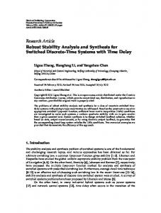
paper with a discussion. 2. Model for Robust Stability in 4C Based Teleoperation 2. Model for Robust Stability in 4C Based Consider the generic teleoperation setupTeleoperation depicted in Figure 1, consisting of an exchange of signals through a communication channel between the master side (left) and the slave side (right). The master Consider the generic teleoperation setup depicted in Figure 1, consisting of an exchange of side is formed of the plant 1/Pm and the controller Km . The plant is modelled as a mechanical signals through a communication channel between the master side (left) and the slave side (right). system with coordinates (positions) given by the n ˆ 1 vectors xm , xs . In the Laplace domain, if The master side is formed of the plant 1/Pm and the controller Km. The plant is modelled as a . xm p0q “ x m p0q “ 0, we have: mechanical system with coordinates (positions) given by the n × 1 vectors xm, xs. In the Laplace domain, if xm (0) xm (0) 0, we have: Pm psqXm psq :“ Fm psq, Ps psqXs psq :“ Fs psq (1)
Pm (s) X m (s) : Fm (s), Ps (s) X s (s) : Fs ( s) (1) Note that we use lowercase and uppercase letters for time-domain and Laplace domain Note that we use lowercase and uppercase letters for time-domain and Laplace domain signals, signals, respectively. respectively.
Figure 1. Generic Figure 1. Generic teleoperation teleoperation system. system.
The input of the master plant is the master force f f f mc , where fh is the force applied by the The input of the master plant is the master force fmm “h f h ´ f mc , where fh is the force applied by human operator and fmc is the force from the controller. The plant has two outputs, namely, the ny the human operator and fmc is the force from the controller. The plant has two outputs, namely, the ny signals that send information to the slave (ym) and the nz signals used by the local controller (zm). signals that send information to the slave (ym ) and the nz signals used by the local controller (zm ). On the slave side, fe is the force from the environment. The controller force fsc enters additively On the slave side, fe is the force from the environment. The controller force fsc enters additively in in f s fe f sc . f s “ f e ` f sc . Master and and slave slaveexchange exchangesignals signalsthrough through communication channel. Taking account Master thethe communication channel. Taking intointo account our our theoretical [10],experimental and experimental [11] discussions delay using bounds theUser Internet User theoretical [10], and [11] discussions on delayonbounds theusing Internet Datagram Datagram(UDP), Protocol the delay can be in assumed in a non-restrictive from teleoperation Protocol the(UDP), delay τ(t) can beτ(t) assumed a non-restrictive way fromway teleoperation point of point toofbeview, to be an unknown function time-varying function for which the bounds and on the view, an unknown time-varying for which the upper bounds on upper the magnitude the magnitude and the variation satisfy t 0 : variation satisfy @t ě 0: 0 (t ) h (t ) hmax ,
(t ) h
(2)
Sensors 2016, 16, 593 Sensors 2016, 16, 593
4 of 20 4 of 19
(t ) d 1
(3)
The time-varying delay0 can be described D which ď τptq “ h ` ηptqby ď the hmaxoperator , ď κ ď his a (nonlinear) system used (2) |ηptq| the time domain) in ˇ . ˇany of the equivalent notations: ˇτptqˇ ď d ă 1 (3) y jd (yj) yj y j , (j m, s) . This means that: j j delay can bej described by the operator D which is a (nonlinear) system used (in The time-varying the time domain) in any the equivalent notations: D j py ymd (tof ) D y (t ) : ymi (t m (t )), ysdy jd(t )“D y j(qt )“ : D ys ij(˝ t yj s “ (t ))D j y j , pj “ m, sq . This (4) m m s s means that: where D m, D s are the corresponding master and slave time-delay operators. To simplify matters we ptq “operator Dm ymi ptq :“ pt ´ the τm ptqq,Laplace (4) ysdi ptq domain “ Ds ysi ptqin :“ ythe τs ptqq si pt ´ equivalent also extendymdthe Dymito forms i (in
D
D
D
i
D
D
i
i
i
D
, slave time-delay which simply To simplify means Y jd D m , (DYsj are ) the corresponding Yj Yj where and operators. matters wethat: also j j j master extend the operator D to the Laplace domain in the equivalent forms Yjd “ D j pYj q “ D j ˝ Yj “ D j Yj , Y jd ( s) Y j ( s) Y jd ( s) L y jd (t ) and y jd (t´) ¯ y j (t ) . which simplyj means that: Yjd psq “ D j Yj psq ô Yjd psq “ L y jd ptq j and y jd ptq “ D j y j ptq. We now consider a 4C control scheme in the most general and representative case of delay-dependent schemes. master and and slaveslave exchange, through the communication channel, schemes.Here, Here,thethe master exchange, through the communication velocitiesvelocities or positions and forcesand in both directions. The local controllers defined are in terms of the channel, or positions forces in both directions. The local are controllers defined in appliedofexternal force, external their ownforce, velocity/position (master/slave) and the delayed velocity/position terms the applied their own velocity/position (master/slave) and the delayed and force (slave/master) the other side. the system exchanges positions and forces (see velocity/position and forcefrom (slave/master) fromWhen the other side. When the system exchanges positions Figure 2), the as: be defined as: and forces (seecontrollers Figure 2), Kthe controllers Km, Ks can m, K s can be defined
D
D
C´6 C f h6 f h f mcf mc“CCmmxxmm `CC22ffsdsd`CC 4 x4sdx sd
(5) (5)
Cssxxss ` C C1 x1md C fe5 f e f scf sc“´C C33 ffmd xmd `5 C md ` C
(6) (6)
Figure Figure 2. 2. Local Local controllers controllers in in the the 4C 4C control control scheme.
Following the procedure described in a previous work [11], we remodeled this whole system to Following the procedure described in a previous work [11], we remodeled this whole system to obtain a single feedback loop containing an LTI block and an uncertain time-varying delay block obtain a single feedback loop containing an LTI block and an uncertain time-varying delay block with with the same dimension as the number of the signals exchanged between the master and slave. For the same dimension as the number of the signals exchanged between the master and slave. For this this purpose, we state the following Proposition 1 to obtain the model for 4C-based teleoperation: purpose, we state the following Proposition 1 to obtain the model for 4C-based teleoperation: Proposition 1. A teleoperation setup as described in Figures 1 and 2, given by Equations (1)–(5), can Proposition 1. A teleoperation setup as described in Figures 1 and 2 given by Equations (1)–(5), can be be formulated as a compact model for robust stability analysis using a generic approach (as formulated as a compact model for robust stability analysis using a generic approach (as developed developed in [11]) in the form given by equations Equation (7), Equation (8) and the block diagram in [11]) in the form given by equations Equation (7), Equation (8) and the block diagram in Figure 3: in Figure 3: ΠpsqXpsq D DpsqXpsq ( s) X ( s)“ ´Cpsq C( s)D D( s) X ( s` ) ΦpsqFpsq ( s) F ( s)
with: with:
(7) (7)
Sensors 2016, 16, 593
5 of 19
Sensors 2016, 16, 593
˜ Π“
5 of 20
¸
˜
¸
¸
˜
˜
0 2 Pm ` Cm 0 P C Xm C C I ¨D X “ C C4 2 I,2 D D“ 0 222 m m 011ˆ ,m X “ 0 , C m ,s X m , C ´C 1 2´C3 4 012 ˆ ,2D 0 , 0 Ps` Cs X Ps C s 012 I 2 D2sˆ 2 0 Xs - C1 - C 3 0 22 ¨ ´ ¯T 02ˆ1 1 Pm T ˚ 1 Pm ´ 0 21 ¯ D“˝ T, D 02ˆ1 0 21 11 PPss T
02ˆ2 I2 ¨ Ds
¸ ,
(8)
˛
(8)
˜ ¸ ˜ ¸ Fh ‹ 1 C6 1 ` 0C6 0 Fh ‚ , F , F “ , Φ “ Fe 10 C5 1 ` C5Fe 0
Figure 3. Teleoperation loop.
Figure 3. Teleoperation loop.
Proof: The proof of this proposition is developed in Appendix A.
Proof: The proof of model this proposition is developed A. 2 Remark 1. The described by Equation (7)inisAppendix directly represented by Figure 3, where four time-varying delays channels inherited from Figure 1 are maintained, bearing in mind that they
Remark 1. be The modelindescribed by because Equation (7) is directly by with Figure where four cannot combined a single delay time-varying delaysrepresented do not commute LTI3, systems. time-varying delays channels inherited from Figure 1 are maintained, bearing in mind that they cannot Ideal Transparency Conditions be combined in a single delay because time-varying delays do not commute with LTI systems. Note that, from the teleoperation loop in Figure 3, we can also obtain the zero-delay (D = I
Ideal Transparency Conditions Yd = Y) closed loop dynamics for studying ideal behavior and transparency properties, considering:
1 Note that, from the teleoperation also the zero-delay (D X (s) (sloop ) C (in s) DFigure (s) 3,(swe ) F (scan ) : (s) Fobtain ( s) (9) = I ñ Yd = Y) closed loop dynamics for studying ideal behavior and transparency properties, considering:
That is:
´1 Xpsq “xpΠpsq ` CpsqDpsqq “: ΛpsqFpsq 1 x ΦpsqFpsq ( f f ) f
That is:
m h m 11 h 12 e 1 x ( f xs fe 21 h 22 f e ) s
¸ ˜ ¸ # x f xm “ ∆Λ ´1 ¨ pΛ11 f h ` Λ12 f e q m h with the following values: “ Λ¨ ñ xs fe xs “ ∆Λ ´1 ¨ pΛ21 f h ` Λ22 f e q 11 Ps Cs 1 C6 , 12 C4 C2 Ps 1 C5 with the following values: C C P 1 C , P C 1 C
(9) (10)
˜
1 3 m 6 22 m m 5 pPs `PmC Cm ` P “ C1´ pC C34Pm`CC2 P C5 q 4 s 2 Ps` Λ11 “ Cs 6q C , sΛ12 qC ¨ p1 s q ¨ p1 21
Λ
“ pC ` C P q ¨ p1 ` C q , Λ
“ pP ` C q ¨ p1 ` C q
(10) (11)
m m the impedance 3 mdefinition6can be 22associated 5 21 1 matrix The previous admittance with Z or hybrid ∆Λ “ pPm ` Cm q ¨ pPs ` Cs q ` pC1 ` C3 Pm q pC4 ` C2 Ps q H models:
(11)
fdefinition fh xmatrix Z 22 xm be 12associated xs , The previous admittance can with the impedance Z or hybrid Z 1 C5 1 C6 Z m h (12) 1 H models: fe xs f e Z 21xm 11xs ˜ ¸ ˜ ¸ # fh xm f “ ∆ ´1 ¨ pΛ xm ´ Λ xshq f m 12 e , ∆ Z “ p1 ` C5 q ¨ p1 ` C6 q “Z¨ ñ f hh HZ´ 1 xm 22 f h h11x12 (12) (13) xm ` Λ11 xs q fe xs fxe “ ∆ Z ¨f p´Λ 21 x h x h f 1
s
e
s
21 m
22 e
The ideal transparencyf properties are xusually defined onhthexH` matrix, f “ h f regarding which:
˜
¸
h
xs
˜
“ H¨
¸
m
fe
#
ñ
h
11 m
12 e
xs “ h21 xm ` h22 f e
(13)
Sensors 2016, 16, 593
6 of 19
The ideal transparency properties are usually defined on the H matrix, regarding which: h11 “ h22 “ 0 transparency, h12 ¨ h21 “ ´1 condition set
(14)
Comparing Equations (13) and (14) with Equation (9), we obtain:
h21 “
Λ21 Λ11
12 h11 Ñ 0 ñ ∆Λ Ñ 0 , h12 “ ´ Λ Λ “ ´1 ñ Λ12 “ Λ11
(15)
11
“ 1 ñ Λ21 “ Λ11 , h22 “ 0 ñ Λ11 Λ22 ´ Λ12 Λ21 “ 0 ñ Λ22 “ Λ11
Therefore, these properties can also be analyzed through Λ and Z matrix in the following form: ˜ 1 ∆Z
Transparency and Condition set ” Zideal “
Λ11 ´Λ11
¸ ´Λ11 Λ11
˜ , Λideal “
1 ∆Λ
Λ11 Λ11
Λ11 Λ11
¸ with ∆Λ Ñ 0
(16)
3. Robust Stability for 4C Based Teleoperation Below we apply our previously developed approach to stability under time-varying delay in teleoperation [11,22] to the 4C control scheme. The time-varying delay is an uncertainty that may give rise to instability. To ensure robust stability, of necessity we have to impose some limits on maximum delay and maximum delay variation. Our treatment of time-varying delay is based on an encapsulation described in the literature [29] and adapted by us to a 4C teleoperation setup. This delay encapsulation [29]—based on the concept of the integral quadratic constraint (IQC), which is a powerful framework for robust stability—is combined with input-output stability criteria and µ-analysis and synthesis techniques in order to achieve a final robust stability condition (Theorem 1). Proposition 2. A teleoperation setup, as stated in Proposition 1 and depicted in Figure 3, can be modeled as a negative single-feedback loop containing an LTI block G(s) and an uncertain time-varying delay block D , shown in Figure 4a, with: Gpsq “ DpsqΠ´1 psqCpsq ¨ ˚ ˚ G“˚ ˝
02ˆ2 ´1
´ pPs ` Cs q C1 ´Ps pPs ` Cs q´1 C1
´1
(17)
pPm ` Cm q´1 C4 Pm pPm ` Cm q´1 C4
´ pPs ` Cs q C3 ´Ps pPs ` Cs q´1 C3
pPm ` Cm q´1 C2 Pm pPm ` Cm q´1 C2
02ˆ2
˛ ‹ ‹ ‹ ‚
(18)
Theorem 1. Consider a 4C-based teleoperation system, modeled by Equations (7) and (8), directly represented by Figure 3 and transformed into Figure 4a by Proposition 2. Given G(s) as defined in Equation (15), let φ(s) [29]: ϕpsq “ k ¨
h2max s2 ` c ¨ hmax s h2max s2 ` ahmax s ` k ¨ c
(19)
? ? with k “ 1 ` 1{ 1 ´ d, a “ 2kc where c is any positive real number and delay bounds hmax and where d is as defined in Equations (2) and (3). If necessary, [29] provides extensions of the delay encapsulations by another multipliers ϕ in Equation (19) that deal with great variability. A sufficient condition for stability of the delayed system as described in Figure 4a, with a complex diagonal structured uncertainty, is given by: Γ “ max µ rHpjωqs “ max ρ rHpjωqs ă 1
(20)
Hpsq “: ϕpsq ¨ pI ` Gpsqq´1 Gpsq
(21)
ωPr0,8s
ωPr0,8s
where:
Sensors 2016, 16, 593
7 of 19
Sensors 2016, 16, 593
7 of 20
and where µ p¨q is the structured singular value (SSV) with respect to a repeated complex scalar and where is the structured singular value (SSV) with respect to a repeated complex scalar uncertainty, which is, in turn, equal to ρ p¨q, the spectral radius of a matrix (the maximum of the norms uncertainty, which is, in turn, equal to , the spectral radius of a matrix (the maximum of the of the eigenvalues). norms of the eigenvalues).
Proof. This result is obtained in two ways. First, in applying the loop transformation theorem (the Proof. This result is obtained in two ways. First, in applying the loop transformation theorem (the loop depicted in Figure 4a is4astable if the Figure 4bstable) is stable) and thegain small gain loop depicted in Figure is stable if theloop loop depicted depicted inin Figure 4b is and the small theorem theorem to Figure 4b, whereby k Hpsq k ¨ k ∆ k ă 1, since k ∆ k ď 1 by [29], a sufficient condition to Figure 4b, whereby H ( sL)2 L L L2 1 , since L 1 Lby 2 [29], a sufficient condition is 2 2 2 is k Hpsq k L2 ă 1. Second, using the µ-techniques for robust stability [30] we can interpret Figure 4b H ( s) L 1 . Second, using the μ-techniques for robust stability [30] we can interpret Figure 4b as a 2 as a nominal system H(s) connected to a dynamic or complex uncertainty ∆ that is actually diagonal nominal system H(s) connected to a dynamic or complex uncertainty Δ that is actually diagonal (more details are given in [11]). 2 (more details are given in [11]).
Remark Remark 2. As a 2.prerequisite for for robust stability, mustfirst first satisfy nominal stability. Hence, H(s) As a prerequisite robust stability, we we must satisfy nominal stability. Hence, H(s) mustverify verify real must be Hurwitz-stable, that that is, all λi λeigenvalues must be Hurwitz-stable, is, the all the i eigenvalues must real i i1“ n1 .. . . n . pλ i q0ă 0i, @i, i
(a)
(b)
Figure 4. (a) LTI system with time-varying delay in the feedback loop; (b) Loop transformation.
Figure 4. (a) LTI system with time-varying delay in the feedback loop; (b) Loop transformation. This frequency approach based on IQCs combined with μ-analysis and synthesis techniques is a framework for robust Therefore, using the µ-analysis stability condition of Equationtechniques (20) Thispowerful frequency approach basedstability. on IQCs combined with and synthesis is based on the system in Equation (21), for any delay satisfying Equations (2) and (3) and for some a powerful framework for robust stability. Therefore, using the stability condition of Equation (20) designed closed-loop (non-delayed) dynamic in G, we can ensure robust stability under based ontime-varying the system in Equation (21), for any delay satisfying Equations (2) and (3) and for delays. some designed closed-loop (non-delayed) dynamic in G, we can ensure robust stability under 4. Haptic Teleoperation Case Study time-varying delays. The previous 4C architectural framework was applied to remote teleoperation between
4. Haptic Teleoperation Case Study master and slave haptic devices located in laboratories in the University of Vigo and the University of Manchester.
The previous framework was and applied to remote teleoperation betweenWe master and Below 4C we architectural describe the details of the setup of master and slave device identification. slave haptic in laboratories in the University of Vigo and theus University of Manchester. thendevices describe located a scaled control scheme γ-4C in which the stability factor γ lets obtain a practical andwe internally stable teleoperation, where all the controllers are proper We then Below describe thesolution details to ofInternet-based the setup and of master and slave device identification. (without differentiators), as is usual in classical solutions. Further sections will describe simulations describe a scaled control scheme γ-4C in which the stability factor γ lets us obtain a practical and and experimental results. internally stable solution to Internet-based teleoperation, where all the controllers are proper (without The master and slave sides consist of two Phantom Omni haptic devices manufactured by differentiators), is usual in solutions. Further sections will describe simulations and SensAble as Technologies Inc.classical (Wilmington, MA, USA). In terms of degree of freedom (DoF), these experimental results. devices have 6-DoF position sensing and 3-DoF force actuation. To focus on the robust stability we limited movements 1-DoF—rather than multi-DoF—using the first devices rotational manufactured coordinate Theissue, master and slave sidestoconsist of two Phantom Omni haptic by (the base rotation) as the free DoF. In this way, the two Omnis rotated around their vertical axes, SensAble Technologies Inc. (Wilmington, MA, USA). In terms of degree of freedom (DoF), these while the shoulder, elbow and stylus were blocked. devices have 6-DoF position sensing and 3-DoF force actuation. To focus on the robust stability issue, Thus, the master and slave positions were (xm, xs), the sensed Omni base angles in radians (rad). we limited than multi-DoF—using thefor first rotational coordinate (the Themovements actuations areto(fm1-DoF—rather , fs), which are the torque inputs to the motors vertical axis rotation in base rotation) asunits the free DoF. thisaccess way,tothe two Omnis machine (we did notIn have physical units). rotated around their vertical axes, while the shoulder, elbow and stylus were blocked. Thus, the master and slave positions were (xm , xs ), the sensed Omni base angles in radians (rad). The actuations are (fm , fs ), which are the torque inputs to the motors for vertical axis rotation in machine units (we did not have access to physical units). We concentrated on 1-DoF movements around a fixed position (the “zero” of the Omnis). Although the Omnis are robotic nonlinear systems, given the linearization principle, it was expected that the local dynamics from forces to positions could be captured as is usual by models in the form
Sensors 2016, 16, 593
8 of 19
Gi (s) = 1/(s(Ms + B)) [31]. Note that here, for simplicity sake, we use the terms “forces” and “positions” to denote torques and angles. Note also that, since the forces are in machine units, the inertia-mass M and friction B coefficients were given in machine or virtual units. Before identifying the models Gi (s), our experiments showed that there was a deadzone or static friction at the force inputs. This meant that the effective force fe f was smaller than the applied or written force fi . This effect can be modelled by a deadzone function fef = DZ(fi ; Dpos , Dneg ) in the form: ! f e f “ max
) 0,
f i ´ D pos
! f i ą 0, f e f “ min
if
) 0,
f i ` Dneg
if
fi ă 0
(22)
Although this static friction slightly damaged linearity, producing small steady-state errors, this was easily mitigated by pre-compensation at input by an inverse function in the form fi = DZ(f ; ´Dpos , ´Dneg ) with negative values ´Dpos , ´Dneg . If the deadzone (asymmetric) widths Dpos , Dneg were estimated well, the composition of these two functions would give rise to the identity, fef = f, thus linearizing the system. After linearizing the devices by deadzone compensation, the linear models Gi (s) = 1/(s(Ms + B)), were obtained, by a standard procedure [24] applied in closed -loop (proportional controller) square and triangular references, recording force inputs and position outputs and performing standard least-squares identifications of M, B. The results (in machine units, m.u.) were: M “ 0.00118 pm.u.q B “ 0.0199 pm.u.q
(23)
Therefore, for the teleoperation setup described in Figure 1 formed of two identical OMNI Phantoms as the master and slave systems, for each DoF, the linearized dynamic models were: Pm “ Ms2 ` Bs “ Ps “ P
(24)
Seeking a practical solution to Internet-based teleoperation, we fine-tuned a scaled 4C control scheme γ-4C. We also imposed internal stability, that is, the closed-loop system had to be Hurwitz-stable. The operator and environment were modelled as external forces. These requirements were met in the scheme depicted in Figures 1 and 2 and given by Equations (1)–(5), with master and slave systems as in Equation (24) and with the controllers in Equation (5) defined in the following form:
C4 psq “
For Cm “ Cs “ K ą 0 and γ ą 1 : C1 psq “ Cm , C2 “ ´ γ1 , C3 “ 1, C5 “ C6 “ K1
´ Cγs ,
(25)
The Λ and Z matrix in this γ-4C scheme with controllers given by Equation (25) take the values: ˜ Λpsq “
p1`K1 q ∆Λ
pP ` Kq pP ` Kq
1 γ
¨ pP ` Kq pP ` Kq
¸ ´ ¯ ∆Λ “ pP ` Kq2 ¨ 1 ´ γ1
,
(26) ˜ Z“
1 p1`K1 q2
pP ` Kq ´ pP ` Kq
´ γ1
pP ` Kq pP ` Kq
¸
Note that the control parameters in Equation (5) with the values selected in Equation (25) were not eight independent controllers. Due to the transparency restriction requirements, there were ultimately only a minimum of two DoFs in the design: the gain K and the coefficient γ (K’ can be zero). The gain K was the only parameter that directly influenced the closed-loop poles (∆Λ = 0) in the non-delayed case, as seen in Equation (26). The value k > 0 was necessary to ensure non-delayed system stability. We could thus tune k > 0 from pole-placement principles, bearing in mind that the feedback loop would be affected by a (time-varying) delay. As for the coefficient γ, this ideally should be set to γ = 1 to ensure perfect transparency, but to avoid singularity in the feedback loop impedance (admittance) matrix, it
Sensors 2016, 16, 593
9 of 19
was set to γ > 1. For greater transparency, γ should be as close as 1 as possible, but has to be greater than 1 to ensure robust stability and loop well-posedness. Remark 3. If γ = 1 + ε, with ε Ñ 0, the teleoperation system with the controllers defined by Equation (25) verify the transparency-optimized conditions for zero delay Equation (16). But in the ideal case ε = 0, the impedance matrix Equation (12) loses rank and thus the admittance model Equation (10) is thus not well-defined (ill-posed). Remark 4. To avoid the previous issue, the γ factor in Equation (25) can be selected to verify well-posedness and robust stability conditions under Internet time-varying delay, while maintaining the transparency properties of the system as much as possible. This control scheme therefore gives internal stability and a practical solution to the trade-off between performance and stability under time-varying delay. Remark 5. The proposed control scheme in Figures 1 and 2 as given by Equation (5) allows proper controllers in Equation (25) to be selected based on ideally optimized transparency, that is, they do not contain single or double differentiators like classical 4C solutions and so avoid negative effects with noise. See the explanation in Appendix B. Remark 6. The controllers defined in Equation (25) also provide robust stability and performance against parametric uncertainty. The closed-loop poles are now given by (Mm s2 + Bm s + K) (Ms s2 + Bs s + K) = 0 and, consequently, for zero delay, the system will be stable iff K, Mm,s = M ˘ ∆M , Bm,s = B ˘ ∆B >0. These remarks are further analyzed in the following sections. 5. Analysis and Simulation Results We first describe a simulation case for use with Simulink and Matlab, considering linear dynamic models for the master and slave, the rounded identified values given by M = 0.001, B = 0.02 and the controllers as stated in Equation (25), with K = 0.1 and K’ = 0. To justify choosing this control scheme based on performance criteria, using this simulation case and applying zero delay, we compared our scheme with some frequently used two- and three-channel (2C and 3C) control schemes. These schemes can be obtained by canceling certain controller parameters in Equation (25), as shown in Table 1. Table 1. Control Schemes (Pm = Ps = P = 0.001s2 + 0.02s, Cm = Cs = K = 0.1, C5 = C6 = K’ = 0). C1
C2
C3
∆Λ
C4
PE
K
0
0
´K
FP
0
0
1
´K
PF
K
´1
0
0
3C-i
K
´1
0
´K
3C-ii
K
0
1
´K
4C (γ = 1.07)
K
´1/γ
1
´K/γ
P2
` 2PK si = 0, ´20, ´10 ˘ 10i P2 ` PK ` K2 si = ´18.7 ˘ 5i, ´1.3 ˘ 5i P2 ` PK ` K2 si = ´18.7 ˘ 5i, ´1.3 ˘ 5i P2 ` PK si = 0, ´20, ´10, ´10 P2 ` PK si = 0, ´20, ´ ´10, ´10 ¯ pP ` Kq2 ¨ 1 ´ γ1 si = ´10, ´10, ´10, ´10
∆Λ Λ ˆ
P`K ˆ K P`K P ˆ P`K ˆ K P`K ˆ K P`K ˜ P`K P`K P`K
˙ K P`K ˙ K P`K ˙ P P`K ˙ P`K P`K ˙ K P`K ¸ 1 γ pP ` Kq P`K
Note that the 4C scheme results were obtained for γ = 1.07 « 1 to avoid singularities. The selected value in K provided an adequate time response by fixing equal and real closed-loop poles, that is, the linear model of the system had critical damping and so did not overshoot. Performance can be studied by simulations that apply a simulated sine reference force (fh )—like the force imposed by a human operator—to move the master. The slave will follow the master in free motion in the interval t = (0, 10) and (18, 30) s and with an environment step force fe simulated from
Sensors2016, 2016,16, 16,593 593 Sensors Sensors 2016, 16, 593 Sensors 2016, 16, 593
1010ofof2019 10 of 20 10 of 20
Note that the 4C scheme results were obtained for γ = 1.07 ≈ 1 to avoid singularities. The t = 10 s and t = 18 s Note that the operator and environment are not assumed to be in contact or to Note thatinthe 4C scheme results were = 1.07 ≈ 1 and to avoid singularities. The selected value K provided an adequate timeobtained responsefor by γfixing equal real closed-loop poles, Note that the 4C scheme results were obtained for γ = 1.07 ≈ 1 to avoid singularities. The be passive. selected K provided an adequate time response fixing equal real closed-loop poles, that is, thevalue linearinmodel of the system had critical dampingby and so did not and overshoot. selected in K provided an adequate response byfor fixing equal and real closed-loop poles, The value best results for tracking propertiestime were obtained the schemes which approximated the thatPerformance is, the linear can model of the system had critical damping and so did not overshoot. be studied by simulations that apply a simulated sine reference force (fh)—like that is, the linear model of the(γ-4C) systemor, had critical damping did3Cii) not overshoot. ideal transparency conditions at least, the schemesand (PE,so3Ci, in which conditions were Performance can be studied by simulations apply a The simulated sinefollow reference force (fhin )—like the force imposed by a human operator—to movethat the master. slave will the master free Performance can bestate studied that apply a simulated sineare reference (fh)—like achieved in the steady (s Ñby 0).simulations The simulation results, for brevity, shown force only for these the force by at =human the master. The slave step will follow master in free motion in imposed the interval (0, 10)operator—to and (18, 30) smove and with an environment force fethe simulated from the force (Figures imposed 5–8). by a human operator—to move the master. Thestability slave will the master in free schemes Only the γ-4C scheme provided internal to follow the system. Because the motion in the interval t = (0, 10) and (18, 30) s and with an environment step force f e simulated from t = 10 s and t = 18 s Note that the operator and environment are not assumed to be in contact or to motion in the interval t = (0, 10) and 30) origin, s and with an environment step force fe simulated from other schemes have a closed-loop pole(18, at the without external forces, some states of the system t =passive. 10 s and t = 18 s Note that the operator and environment are not assumed to be in contact or to be t = 10 s to and = 18 svalue Note (in that thecase operator environment areexample, not assumed be in 9a. contact or to tended thet same this xm = xand not to zero, for PE intoFigure However, s ) but be passive. be passive. the γ-4C scheme in Figure 9b, without external forces, drove the master and slave to their zero states. x 10 •3
Master Slave
0.5
Master Slave Master Slave
3 4
0.3 0.2 0.3
3 1 2 2 0 1
1 •1 0
0.2 0.1 0.2
0 •2•1
0.1 0 0.1
•1 •3•2
0
•2 •4•3
0 0 •0.1 •0.1
x 10
4 2 3
0.4 0.3 0.4
•0.1
x 10
•3
Forces (m.u.) Forces (m.u.) Forces (m.u.)
Positions (rad) Positions (rad) Positions (rad)
0.5 0.4 0.5
Fm Fs FhFm FeFs Fm Fh Fs Fe Fh Fe
•3
4
5
10
15
20
25
•3 0 •4
30
Time (s) 0
5
10
15
20
25
•4
30
5
10
15
20
25
30
Time (s) 0
5
10
15
20
25
Time15 (s) Time15(s) 20 25 30 0 5 10 20 25 (a) (b) Time (s) Time (s) (a) (b) Figure 5. Simulated sine 0, d = 0. (a) Positions; (a) reference force: PE control scheme with hmax = (b) 0
5
10
30 30
Figure 5. Simulated sine reference force: PE control scheme with hmax = 0, d = 0. (a) Positions; (b) Forces. Figure 5.5. Simulated Simulatedsine sine reference force: PE control scheme with =hmax = 0. (a) (b) Positions; Figure reference force: PE control scheme with hmax 0, d = =0. 0, (a)dPositions; Forces. (b) Forces. (b) Forces. x 10 •3
Master Slave Master Slave Master Slave
1 1 0.8
1
6
6 4
2
Forces (m.u.) Forces (m.u.) Forces (m.u.)
Positions (rad) Positions (rad) Positions (rad)
•3
x 10
•3
Fm Fs Fh Fm Fe Fs Fm Fh Fs Fe Fh Fe
4
0.8 0.6 0.8 0.6 0.4 0.6
4 2
0
0.4 0.2 0.4
2 0
•2
0.2 0 0.2
•4
0 •0.2
6
x 10
0 •2 •2 •4
0
•6
0 •0.2
5
10
15
20
25
30
Time (s)
•0.2 0
5
10
15
20
25
30
•4 0 •6 •6
5
10
15
20
25
30
Time (s) 0
5
10
15
20
25
30
Time15(s) 20 25 30 0 5 10 20 25 30 (a)Time15(s) (b) Time (s) Time (s) (a) (b) Figure 6. Simulated sine(a) reference force: 3C-i control scheme with hmax = (b) 0, d = 0. (a) Positions; 0
5
10
Figure 6. Simulated Simulatedsine sine reference force: control scheme = 0. (a) (b) Positions; (b) Forces. Figure 6. reference force: 3C-i 3C-i control scheme with h with = 0,hmax d = =0. 0, (a)dPositions; Forces. Figure 6. Simulated sine reference force: 3C-i control scheme max with hmax = 0, d = 0. (a) Positions; (b) Forces. (b) Forces. x 10 •3
6
Master Slave Master Slave Master
1 1 0.8 1
6 4 6
•3
Fm Fs Fh Fm Fe Fs Fm Fh Fs Fe Fh
2 4
Forces (m.u.) Forces (m.u.) Forces (m.u.)
Positions (rad) Positions (rad) Positions (rad)
•3
x 10
4
Slave
0.8 0.60.8 0.6 0.40.6 0.4 0.20.4
Fe
2 0 2 0
•2 0
0.2 00.2
•2
•4 •2
0 •0.2 0 •0.2 0 •0.2
x 10
•4 5 0
10 5
15 10
20
Time (s) 15
25 20
•6 •4 0 •6
30 25
30
•6 0
5
10 5
15 10
20
Time (s) 15
25 20
30 25
30
15(s) 20 25 30 0 5 10 15 (s) 20 25 30 (a)Time (b)Time Time (s) Time (s) (a) (b) Figure sine(a) reference force: 3C-ii control scheme hmax (b) = 0, d = 0. (a) Positions; Figure7.7. Simulated Simulated sine reference force: 3C-ii control scheme with hwith max = 0, d = 0. (a) Positions; (b) Forces. 0
5
10
Figure 7. Simulated sine reference force: 3C-ii control scheme with hmax = 0, d = 0. (a) Positions; (b) Forces. Figure 7. Simulated sine reference force: 3C-ii control scheme with hmax = 0, d = 0. (a) Positions; (b) Forces. (b) Forces.
Positions (rad) Positions (rad)
0.6 0.4
Fe
0.03 0.03
Forces (m.u.) Forces (m.u.)
0.4 0.2 0.2 0 0 •0.2 •0.2 •0.4 •0.4 •0.6
0.01 0.01 0 0 •0.01 •0.01
Sensors 2016, 16, 593 •0.6 •0.8 Sensors 2016, 16, 593 5
10
15
20
25
5
10
Time15 (s) Time (s)
20
25
0.8
30
0 0.050
30 Master Slave
(a) (a)
0.6
11 of 19 11 of 20
•0.02 •0.02
•0.8 •1
•1 0 0
0.02 0.02
5 5
10 10
15
Time15 (s) Time (s)
20 20
25 25
Fm Fs Fh Fe
(b) (b)
0.04
30 30
0.03
Forces (m.u.)
Positions (rad)
0.4 Figure 8. Simulated sine reference force: γ-4C control scheme with hmax = 0, d = 0. (a) Positions; Figure 8. Simulated sine reference force: γ-4C control scheme with hmax = 0, d = 0. (a) Positions; 0.2 0.02 (b) Forces. 0 (b) Forces. 0.01 •0.2
The•0.4 best results for tracking properties were obtained0 for the schemes which approximated the The•0.6 best results for tracking properties were obtained for the schemes which approximated the •0.01 ideal transparency conditions (γ-4C) or, at least, the schemes (PE, 3Ci, 3Cii) in which conditions ideal transparency conditions (γ-4C) or, at least, the schemes (PE, 3Ci, 3Cii) in which conditions •0.8 were achieved in the steady state (s → 0). The simulation results, for brevity, are shown only for •0.02 •1 were achieved in the10 steady state (s →25 0). The simulation results, for brevity, are shown only for 0 5 15 20 30 0 5 10 15 20 25 30 these schemes (Figures 5–8). Only the γ-4C scheme provided internal stability to the system. Because Time (s) Time (s)to the system. Because these schemes (Figures 5–8). Only the γ-4C scheme provided internal stability the other schemes have a closed-loop pole at the origin, without external forces, some states of the (b)forces, some states of the the other schemes have a(a) closed-loop pole at the origin, without external system tended to the same value (in this case xm = xs) but not to zero, for example, PE in Figure 9a. system tended to the same value (in this case xm = xs) but not to zero, for example, PE in Figure 9a. Figurethe Simulated sinein reference force: γ-4C control control scheme with max 0, (a) Positions; Positions; However, γ-4C scheme Figure 9b, without external forces, drove the master slave to their Figure 8.8. Simulated sine reference force: γ-4C scheme with hhmax == 0, dd == 0.0.and (a) However, the γ-4C scheme in Figure 9b, without external forces, drove the master and slave to their (b)Forces. Forces. zero (b) states. zero states. 0.4 The best results for tracking properties Master were obtained for the schemes which approximated the 0.4 Slave 0.3 Master ideal0.3transparency conditions (γ-4C) or, at Slave least, the schemes (PE, 3Ci, 3Cii) in which conditions 0.2 were0.2 achieved in the steady state (s → 0). The simulation results, for brevity, are shown only for 0.1 0 these0.1schemes (Figures 5–8). Only the γ-4C scheme provided internal stability to the system. Because 0 •0.1 the other schemes have a closed-loop pole at the origin, without external forces, some states of the •0.1 •0.2 •0.2 system tended to the same value (in this case xm = xs) but not to zero, for example, PE in Figure 9a. •0.3 •0.3 However, the γ-4C scheme in Figure 9b, without external forces, drove the master and slave to their •0.4 •0.4 •0.5 zero•0.5 states. 0.4
Master Slave Master Slave
0.4 0.3 0.3 0.2
0.1 0
Positions (rad) Positions (rad)
Positions (rad) Positions (rad)
0.2 0.1
0 •0.1
•0.1 •0.2 •0.2 •0.3 •0.3 •0.4 •0.4 •0.5 •0.5
0
0.5
1
0
0.5
1
0.4
2
2.5
3
0
0.5
1
2
2.5
3
0
0.5
1
(a) (a)
0.3 0.2
0.4
Master Slave
1.5 Time (s) 1.5 Time (s)
2
2.5
3
2
2.5
3
(b) (b)
0.3
Master Slave
Figure 9. Simulatedf fh==f fe== 00 with with hmax ==0,0,0.2 d = 0. Positions. (a) PE; (b) γ-4C. Figure Positions.(a) (a)PE; PE;(b) (b)γ-4C. γ-4C. Figure9.9.Simulated Simulatedhfh = efe = 0 with hhmax max = 0, 0.1 dd==0.0.Positions. Positions (rad)
0.1
Positions (rad)
1.5 Time (s) 1.5 Time (s)
0
0
Furthermore, it may happen that, for some input forces as used in remote teleoperation, the •0.1 used in in remote remote teleoperation, teleoperation, the Furthermore, it may happen that, for some input forces as used •0.2 and slave positions are not bounded for systems without internal stability, although position master although position master •0.3 and slave positions are not bounded for systems without internal stability, although tracking is accomplished—for instance, one of the schemes in Figure 10 and the solution given for •0.4 tracking is accomplished—for instance, one of the schemes in Figure 10 and the solution given for tracking is accomplished—for instance, one of the schemes in Figure 10 and the solution given for the the 4C •0.5 scheme in Figure 11. thescheme 4C scheme in Figure 4C in Figure 11. 11. •0.1 •0.2 •0.3 •0.4 •0.5
0
0.5
1
2
2.5
0
3
Master Slave Master Slave
(a)
10 10
0.5
1
0.06 0.06 0.05 0.05 0.04 0.04 0.03 0.03 0.02 0.02 0.01 0.01 0 0 •0.01 •0.01 •0.02 •0.02 •0.03 •0.03 •0.04 •0.04
1.5 Time (s)
2
2.5
Forces (m.u.) Forces (m.u.)
3
Fm Fs Fm Fh Fs Fe Fh Fe
(b)
Figure 9. Simulated fh = fe = 0 with hmax = 0, d = 0. Positions. (a) PE; (b) γ-4C.
8 8
Positions (rad) Positions (rad)
1.5 Time (s)
6 Furthermore, it may happen that, for some input forces as used in remote teleoperation, the 6 master4 and slave positions are not bounded for systems without internal stability, although position 4 tracking is accomplished—for instance, one of the schemes in Figure 10 and the solution given for 2 the 4C2 scheme in Figure 11. 0 0 0 0
5 5
10 10
15
Time15 (s) Time (s)
20 20
25 25
(a) (a)
10
30 Master 30 Slave
0 0.060
5 5
10 10
0.05
15
Time15 (s) Time (s)
20 20
25 25
(b) (b)
0.04
30 Fm 30 Fs Fh Fe
Forces (m.u.)
Positions (rad)
0.03 8 Figure 10. Simulated ramp-step reference force: PE control scheme with hmax = 0, d = 0. (a) Positions; Figure 10. 10. Simulated Simulated ramp-step ramp-step reference reference force: force: PE PE control control schemewith withhhmax = = 0, d = 0. (a) Positions; 0.02 Figure scheme max 0, d = 0. (a) Positions; (b) Forces. 0.01 6 (b) Forces. Forces. (b) 0 4
•0.01 •0.02
2
•0.03 •0.04
0
0
5
10
15
Time (s)
(a)
20
25
30
0
5
10
15
20
25
30
Time (s)
(b)
Figure 10. Simulated ramp-step reference force: PE control scheme with hmax = 0, d = 0. (a) Positions; (b) Forces.
Sensors 2016, 16, 593 593 Sensors 2016, 16, 593
12 of 20 19 12 of 20 0.14 Master Slave Master Slave
1.5 1.5
0.12 0.1 0.1 0.08
1
Forces (m.u.) Forces (m.u.)
Positions Positions (rad)(rad)
1
Fm Fs Fm Fh Fs Fe Fh Fe
0.14 0.12
0.5 0.5 0 0 •0.5
0.08 0.06 0.06 0.04 0.04 0.02 0.020 •0.020
•0.5
•0.02 •0.04
•1
•0.04 •0.06
•1 0
5
10
0
5
10
15
Time (s) 15
20
25
30
•0.06 0
5
10
20
25
30
0
5
10
15
Time (s) 15
20
25
30
20
25
30
Time (s) (b) (b)
Time (s) (a) (a)
Figure 11. Simulated ramp-step reference force: γ-4C control scheme with hmax = 0, d = 0. (a) Positions; Figure 11. ramp-step reference reference force: force: γ-4C γ-4Ccontrol controlscheme schemewith withhhmax = = 0, d = 0. (a) Positions; (b) Forces. Figure 11. Simulated Simulated ramp-step max 0, d = 0. (a) Positions; (b) Forces. (b) Forces.
Finally, referring back to Remark 6, we used the γ-4C controllers defined in Equation (25) with Finally, referring back to Remark 6, we used the γ-4C controllers defined in Equation (25) with M 2(25) Finally, back to Remark wenow usedthe theslave γ-4Cmodel controllers definedasin P Equation master plant referring as in Equation (24), except6,that was defined s 2with Bs . s MM 2 2 s ` 2Bs. The. 3 master plant as in Equation Equation (24), (24), except except that that now now the theslave slavemodel modelwas wasdefined definedas asPsP“ s 2 Bs s 3 The results canseen be seen in Figure 12. Due thethat fact the thatmodels the models different, the3 master and results can be in Figure 12. Due to thetofact were were different, the master and slave The results can befrom seenthe in Figure Due to the factand thatlocal the models were different, the master and slave forces—obtained from the12. external forces proportional controllers—were also forces—obtained external forces and local proportional controllers—were also different in slave forces—obtained from the external forces and local proportional controllers—were also different in order to accomplish position tracking. order to accomplish position tracking. different in order to accomplish position tracking. 0.06
Master Slave Master Slave
0.8
0.05 0.04
0.6 0.4
0.04 0.03
0.4 0.2
0.03 0.02
0.20 •0.20 •0.2 •0.4 •0.4 •0.6
0.02 0.01 0.010 •0.010 •0.01 •0.02
•0.6 •0.8
•0.02 •0.03
•0.8 •1 •1
Fm Fs Fm Fh Fe Fs Fh Fe
0.06 0.05
ForcesForces (m.u.)(m.u.)
Positions Positions (rad)(rad)
0.8 0.6
0
5
10
0
5
10
15 Time (s) 15 Time (s)
(a) (a)
20
25
30
20
25
30
•0.03 •0.04 •0.04
0
5
10
0
5
10
15 Time (s) 15 Time (s)
(b) (b)
20
25
30
20
25
30
Figure 12.Simulated Simulatedsine sine reference force: control scheme, Ps ≠hmax P, with = 0, d = 0. Figure 12. reference force: γ-4Cγ-4C control scheme, Ps ‰ P, with = 0, d h=max 0. (a) Positions; Figure 12. Simulated sine reference force: γ-4C control scheme, Ps ≠ P, with h max = 0, d = 0. (a) (b) Positions; Forces. (b) Forces. (a) Positions; (b) Forces.
Once the performance of the different schemes was analyzed, we studied stability when the Once the the performance of the schemes was we studied stability when when the the Once performance of the different different was analyzed, analyzed, we time-varying delay was considered. The ideaschemes was to maintain as much asstudied possiblestability the ideal tracking time-varying delay was considered. The idea was to maintain as much as possible the ideal tracking time-varying delay was considered. idea was as much asby possible the ideal tracking properties obtained by the standard The controllers in to themaintain 4C control scheme increasing, by means of properties obtained by the the standard standard controllers controllers in in the the 4C 4C control scheme by increasing, increasing, by by means means of of properties obtained by control scheme by the γ factor, the stability margin in practical conditions, that is, when there was time-varying delay the γ the there was time-varying delay in the γ factor, factor, the stability stabilitymargin marginininpractical practicalconditions, conditions,that thatis,is,when when there was time-varying delay in signals transmission. signals transmission. in signals Oncetransmission. the non-delayed part of the master and slave dynamics were fixed (including the gain K), Once the part of of the master master and slave slave dynamics dynamics were were fixed fixed (including (including the the gain gain K), K), the non-delayed non-delayed part only Once γ remained to be chosen. Allthe the delay and uncertainty was characterized by two measures: the only γ remained to be chosen. All the delay uncertainty was characterized by two measures: the only γ remained be chosen. All the delay uncertainty was characterized by two measures: the maximum delay hto max and the maximum delay rate d. maximum delay hhmax andthe themaximum maximum delayrate rated.d. 1 maximum delay max and The stability condition in Equation delay (20) is based on the H (s) : (s) I G(s)´ 1G( s) system in The stability condition in Equation (20) is based on the Hpsq “: φpsq ¨ pI ` Gpsqq system in in The stability condition in Equation (20) is based on the H (s) : (s) I G(s)1 GGpsq (s) system Equation Equation (21). (21). The The closed-loop closed-loop (non-delayed) (non-delayed) system system G(s) G(s) only only depended depended on on γ, γ, and and the the “multiplier” “multiplier” Equation (21). The system G(s) only depended on γ, and the “multiplier” φ in Equation Equation (19)closed-loop depended(non-delayed) on hhmax,, d. d. Thus φ in (19) depended on Thus the the condition condition in in Equation Equation (20) (20) took took the the form form max φ in Equation (19) depended on h max, d. Thus the condition in Equation (20) took the form . It is important to emphasize that Equation (20) involves the spectral radius of the , h , d 1 Γ pγ, hmax max , dq ă 1. It is important to emphasize that Equation (20) involves the spectral radius of , hmax , d 1. It is important to emphasize that Equation (20) involves the spectral radius of the frequency response H(s)depending depending maxin , d) in a complex way. Thus, the frequency responseH(jω) H(jω)of of some H(s) on on (γ, h(γ, a complex way. Thus, Equation max ,hd) frequency response H(jω) of some H(s) depending on (γ, h max, d) in a complex way. Thus, Equation (20) had to be treated numerically (not analytically). (20) had to be treated numerically (not analytically). Equation had to be treated numerically (notEquation analytically). There(20) was easy way to with deal Equation with (20) numerically: delay uncertainty was anan easy way to deal (20) numerically: the delay the uncertainty parameters There was an easy way to deal with Equation (20) numerically: delaytheuncertainty parameters (hmax , d) could be discretized in the ranges of interest, and for eachthe discretized value, the (hmax , d) could be discretized in the ranges of interest, and for each discretized value, minimum parameters (h max, d) could be discretized in the ranges of interest, and for each discretized value, the minimum γ could be computed. These computations can be represented in the form of 3D γ could be computed. These computations can be represented in the form of 3D surfaces surfaces and the minimum γ could be computed. These computations can be represented in the form of 3D surfaces
Sensors2016, 2016,16, 16,593 593 Sensors Sensors 2016, 16, 593
13ofof19 20 13 13 of 20
and the designer can use the numerical results to decide, depending on the expected delay and the designer can use the results numericaldecide, resultsdepending to decide,ondepending ondelay the expected delay designer can the use adequate the numerical the expected uncertainty, the uncertainty, tuning of γ totobe included in the controllers. uncertainty, the adequate tuning of γintothe becontrollers. included in the controllers. adequate tuning of γ to be included The stability analysis could be assessed applying Theorem 1 and using Matlab. In all cases it The stability analysis analysiscould couldbe be assessedapplying applying Theorem 1 and using Matlab. In cases all cases it The Theorem 1 and using Matlab. In all it had had to stability be proved, firstly, that assessed the system verified the nominal stability condition given in had to be proved, firstly, that the system verified the nominal stability condition given in to be proved, the system the13, nominal stability condition given in Equation (22). Equation (22).firstly, Here that we show, brieflyverified as Figure the effect on stability (from the results on SSV) of Equation (22). Here weasshow, briefly Figure the effect on stability (from theofresults on SSV) of Here we show, briefly Figure theaseffect on 13, stability results SSV) different bounds different bounds on the delay, 13, fixing the stability factor(from at γ the = 12, whichonwas the value selected for different bounds on the delay, fixing the stability factor at γ = 12, which was the value selected for on the delay, fixing the stability factor at γ = 12, which was the value selected for the experiments the experiments described in the next section. Note that the delay variation was the most critical the experiments described in the next Note that the delay wasaspect the most critical described in the next thatsection. delay the variation most critical of stability. aspect of stability. Thesection. results Note depicted inthe Figure 14variation show thewas minimum value of the stability factor γ aspect of stability. The depicted in Figure 14 show theofminimum value of the stability factor γ The results depicted inresults Figure 14 showof the minimum value the stability factor γ (z axis) (z axis) needed to ensure the stability the system given the bounds on the delay (hmax , d).needed to (z axis) the needed to ensure stability ofthe thebounds system on given bounds ensure stability of thethe system given thethe delay (hmax ,on d).the delay (hmax, d). 2.5 2.5
2 hmax = 0.5s, d = 0.95 hmax = 0.5s, d = 0.95
2
hmax = 0.5s, d = 0.75 hmax = 0.5s, d = 0.75
Upperbound on mu Upperbound on mu
1.5 1.5
1 1
STABILITY LIMIT STABILITY LIMIT
hmax = 3s, d = 0.45 hmax = 3s, d = 0.45
0.5 0.5
hmax = 0.5s, d = 0.45 hmax = 0.5s, d = 0.45
0 0
10•2 10
•2
10•1 10
•1
100 Frequency 10 Frequency
0
101 10
1
102 10
2
Figure 13. Upper bound on μ for d, h, (t) ≤ 0.01. Figure13. 13. Upper Upperbound boundon onµμfor ford,d,h,h,|η(t)| (t) ≤ď0.01. Figure 0.01.
Figure 14. γmin (z axis) needed to ensure stability given the delay bounds. Figure 14. γmin (z axis) needed to ensure stability given the delay bounds. Figure 14. γmin (z axis) needed to ensure stability given the delay bounds.
6. Experimental Results 6. Experimental Results 6. Experimental Results In order to test the above simulation results, real experiments were conducted from the haptic In order to test the above simulation results, real experiments were conductedtofrom the haptic teleoperation case as described above. Thereal Omni devices were the the computer In order to teststudy the above simulation results, experiments wereconnected conducted from haptic teleoperation case study as described above. The Omni devices were connected to the computer through a FireWire connection. The computers contained the local controllers implemented under teleoperation case study as described above. The Omni devices were connected to the computer through a FireWire connection. The control computers contained the localmachine controllers implemented under Matlab/Simulink and Quarc real-time software as a real-time for the experiments. The through a FireWire connection. The computers contained the local controllers implemented under Matlab/Simulink and Quarc real-time control software as a real-time machine for the experiments. Quarc software managed thereal-time interfacecontrol with the haptic device using Quarc Phantom Omni software Matlab/Simulink and Quarc software as a real-time machine for the experiments. The Quarc software managed the interface with the haptic device using Quarc Phantom Omni The Quarc software managed the interface with the haptic device using Quarc Phantom Omni software and also collected and saved all exchanged data. The sampling period in the experiments software and also collected and saved all exchanged data. The sampling period in the experiments
Sensors 2016, 16, 593
14 of 19
Sensors 2016, 16, 593 Sensors 2016, 16, 593
14 of 20 14 of 20
Master Master Slave Slave
0.3 0.3 0.2 0.2 0.1 0.1 0 0 •0.1 •0.1 •0.2 •0.2 •0.3 •0.3 •0.4 •0.4 •0.5 •0.5 •0.6 •0.6 •0.7 •0.7 •0.8 •0.8 0 0
Forces (m.u.) Forces (m.u.)
Positions (rad) Positions (rad)
and also collected and saved all exchanged data. The sampling period in the experiments was set was set to 1 millisecond. The two devices were remotely coordinated under programmed force to 1 millisecond. The two devices remotely under programmed force profilesforce like was set to 1 millisecond. The twowere devices werecoordinated remotely coordinated under programmed profiles like the human and environment external forces, and the experimental data validated the the human external forces, and the experimental data validated thevalidated stability and profiles likeand the environment human and environment external forces, and the experimental data the stability and performance results in the theoretical part. performance results in theresults theoretical part. stability and performance in the theoretical part. We describe describeresults resultsfor forthree three experiments. The first experiment (Figure 16) reproduced real We experiments. The first experiment (Figure 16) reproduced real local We describe results for three experiments. The first experiment (Figure 16) reproduced real local teleoperation of the Omni devices at the University of Vigo, artificially increasing a teleoperation of the of Omni the University of Vigo, artificially time-varying local teleoperation the devices Omni at devices at the University of Vigo, increasing artificiallya increasing a time-varying delay between master and slave. The simulation case depicted in with Figure 15first is delay betweendelay masterbetween and slave. The simulation case depicted in Figure is compared this15 time-varying master and slave. The simulation case15depicted in Figure is compared with this first experiment as depicted in Figure 16. experimentwith as depicted Figure 16. as depicted in Figure 16. compared this firstin experiment
5 5
10 10
15 Time 15 (s) Time (s)
20 20
25 25
Fm Fs Fm Fh Fs Fe Fh Fe
0.04 0.04 0.03 0.03 0.02 0.02 0.01 0.01 0 0 •0.01 •0.01 •0.02 •0.02 •0.03 •0.03 •0.04 •0.04 0 0
30 30
5 5
10 10
(a) (a)
15 Time 15 (s) Time (s)
20 20
25 25
30 30
(b) (b)
Figure 15. 15. Local Local teleoperation teleoperation using using linear linear models of master and slave with hmax == 0.5 and 0.45. Figure 0.5sssand andddd===0.45. 0.45. Figure 15. Local teleoperation using linear models of master and slave with hhmax max = 0.5 (a) Positions; (b) Forces. (a) Positions; Positions; (b) (b) Forces. Forces. (a) Forces
0.6 0.6
Master Slave Master Slave
0.4 0.4
Forces (m.u.) Forces (m.u.)
Positions (rad) Positions (rad)
0.2 0.2 0 0 •0.2 •0.2 •0.4 •0.4 •0.6 •0.6 •0.8 0 •0.8 0
5 5
10 10
15 Time 15 (s) Time (s)
20 20
25 25
30 30
0.05 0.05 0.04 0.04 0.03 0.03 0.02 0.02 0.01 0.01 0 0 •0.01 •0.01 •0.02 •0.02 •0.03 •0.03 •0.04 •0.04 •0.05 •0.05 0 0
Forces
5 5
10 10
(a) (a)
15 Time 15 (s) Time (s)
Fm FmFs FsFh FhFe Fe
20 20
25 25
30 30
(b) (b)
Figure 16. Local teleoperation using haptic devices with hmax = 0.5 s and d = 0.45. (a) Positions; Figure 16. max = 0.5 s and d = 0.45. (a) Positions; Figure 16. Local Local teleoperation teleoperation using using haptic haptic devices devices with with hhmax = 0.5 s and d = 0.45. (a) Positions; (b) Forces. (b) Forces. (b) Forces.
Forces (m.u.) Forces (m.u.)
Positions (rad) Positions (rad)
The results were very similar to the simulation results, although the difference between the The results were very similar to the simulation results, although the difference between the linearThe identified used in thetosimulation case and the OMNI nonlinear dynamicbetween with a results models were very similar the simulation results, although the difference linear identified models used in the simulation case and the OMNI nonlinear dynamic with a pre-compensated deadzone can be appreciated. the linear identified modelsEquation used in (22) the simulation case and the OMNI nonlinear dynamic with pre-compensated deadzone Equation (22) can be appreciated. a pre-compensated deadzone Equation (22) can be appreciated. 0.6 Master The second experiment (Figure 17) reproduced real remote teleoperation between the University of 0.6 Slave Master 0.4 Slave Vigo and the University of Manchester using linear models of master and slave like the corresponding 0.4 0.2 simulation model described in Section 5. Here we could analyze the impact of time delays separately 0.2 0 from model uncertainty and nonlinearities issues. The final experiment (Figure 18) tested real remote 0 •0.2 teleoperation between the master haptic device located at the University of Vigo and the slave haptic •0.2 •0.4 located at the University of Manchester. Note that, for implementation over the haptic devices, device •0.4 •0.6 the deadzone was pre-compensated at the input Equation (22) by an inverse function in the form •0.6 •0.8 explained in Section 4. In general, this function caused the system to be more oscillating than the linear 5 10 15 20 25 30 •0.8 0 Time 0 5 10 15 (s) 20 25 30 Time (s) model and to have a small steady-state error. (a) (b) (a) (b) 0.05 0.05 0.04 0.04 0.03 0.03 0.02 0.02 0.01 0.01 0 0 •0.01 •0.01 •0.02 •0.02 •0.03 •0.03 •0.04 •0.04 •0.05 0 •0.05 0
Fm Fs Fm Fh Fs Fe Fh Fe
5 5
10 10
15 Time 15 (s) Time (s)
20 20
25 25
30 30
Figure 17. Remote teleoperation between Vigo and Manchester using linear models of master and Figure 17. Remote teleoperation between Vigo and Manchester using linear models of master and slave. (a) Positions; (b) Forces. slave. (a) Positions; (b) Forces.
Figure 16. Local teleoperation using haptic devices with hmax = 0.5 s and d = 0.45. (a) Positions; (b) Forces.
The results were very similar to the simulation results, although the difference between the linear identified models used in the simulation case and the OMNI nonlinear dynamic with a Sensors 2016, 16, 593 15 of 19 pre-compensated deadzone Equation (22) can be appreciated. 0.05
0.6 Master Slave
0.4
0.03
Sensors 2016, 16, 593 0.2
15 of 20
0.02
Forces (m.u.)
Positions (rad)
Fm Fs Fh Fe
0.04
0
0.01
The second experiment (Figure 17) reproduced real remote teleoperation between the •0.2 University of Vigo and the University of Manchester using linear models of master and slave like the •0.4 corresponding simulation model described in Section 5. Here we could analyze the impact of time 2016, 16, 593 of 20 delays•0.6Sensors separately from model uncertainty and nonlinearities issues. The final experiment15(Figure 18) •0.8 tested real remote teleoperation between haptic at the University 0 5 10 15 20 25 the master 30 The second experiment (Figure 17) reproduced realdevice remotelocated teleoperation between theof Vigo Time (s) and the slave haptic device at the University of Manchester. Note that, for implementation University of Vigo and(a) thelocated University of Manchester using linear models of master and slave like the (b) corresponding simulation model described in Section 5. Here at wethe could analyze the impact of time over the haptic devices, the deadzone was pre-compensated input Equation (22) by an inverse Figure 17. Remote teleoperation between Vigo and Manchester using linear models of master and delays separately from model uncertainty and nonlinearities issues. The final experiment (Figure Figurein17. teleoperation between4.Vigo and Manchester using linear models of master and function theRemote form explained in Section In general, this function caused the system to18) be more slave. (a) Positions; (b) Forces. tested real remote teleoperation between the master haptic device located at the University of Vigo slave. (a) Positions; (b) Forces. oscillating than the linear model and to have a small steady-state error. 0
•0.01 •0.02 •0.03 •0.04 •0.05
5
10
15 Time (s)
20
25
30
and the slave haptic device located at the University of Manchester. Note that, for implementation over the haptic devices, the deadzone was pre-compensated at the input Equation (22) by an inverse 0.06 Master function in the form explained in Section 4.Slave In general, this function caused the system to be more 0.04 oscillating than the linear model and to have a small steady-state error.
0.5
0
Fm Fs Fe Fh
0.02
Forces (m.u.)
Positions (rad)
0.5 Master Slave
•0.5
0.06 Fm Fs Fe Fh
0
0.04
•0.02 0.02 Forces (m.u.)
Positions (rad)
0
0 •0.04
•0.02
•0.5
•1
0
•0.06
0
5
10
15 Time (s)
20
25
30
0
5
10
(a) •1
5
10
20
25
30
(b) •0.06
0
15 Time (s)
•0.04
15 Time (s)
20
25
30
0
5
10
15 Time (s)
20
25
30
Figure18.18.Real Real remote teleoperation between and Manchester using devices. haptic devices. (a) Figure remote teleoperation between Vigo Vigo and Manchester using(b) haptic (a) Positions; (a) Positions; (b) Forces. (b) Forces. Figure 18. Real remote teleoperation between Vigo and Manchester using haptic devices. (a) Positions; (b) Forces.
The data (forces and positions) were exchanged between the master and the slave computers by The data (forces and positions) were exchanged between the master and the slave computers a transmission of UDP packets. Each packet was composed stamps and thecomputers transmitted The data (forces and positions) were exchanged betweenof thetime master and the slave by value by a transmission of UDP packets. Each packet was composed of time stamps and the transmitted with aafixed size ofof68UDP bytes. Figure shows experimental dataand forthe connections Internet transmission packets. Each19packet wassome composed of time stamps transmitted via value value with aa fixed fixedsize sizeof of 68 bytes. Figure 19 some shows some experimental data forviaconnections via with 68 bytes. Figure 19 shows experimental data for connections Internet between Vigo and Manchester. The delay was measured in terms of the round trip time (RTT) Internet between Vigo and Manchester. The delay was measured intheterms oftrip thetime round trip time between Vigo and Manchester. The was delay was ins,terms round (RTT) communication. The maximum delay near hmeasured max = 0.028 with ofvery low variation tested with a (RTT) communication. The maximum was near h 0.028 s, with very low variation communication. The maximum delaydelay was near hmax = 0.028 s,=with very low variation tested with a tested max transmission rate of 1000 packets per second (Figure 19a). The test over the communication channel transmission rate of 1000 packets per second (Figure 19a). The test over thetest communication channel with transmission rate of 1000 per never second (Figure The the communication also arevealed that variations in packets time delay exceeds d19a). = 0.45, as canover be seen in Figure 19b. also revealed that variations in time delay never exceeds d = 0.45, as can be seen in Figure channel alsobe revealed that variations in time delaynetwork never exceeds d = the 0.45,experiment as can be seen in19b. Figure 19b. It should noted thatthat thethecommunication usedin in belongs It should be noted communication network used the experiment belongs to the to the ItGÉANT should be noted that the communication network used in the experiment belongs to the GÉANT pan-European research network,which which quality GÉANT pan-European researchand andeducation education network, hashas veryvery goodgood quality linkagelinkage pan-European research between facilities. between facilities. and education network, which has very good quality linkage between facilities. 60
60
45
delay (msec)
delay (msec)
delay average
50
50 45
40
40
35
35
30
30
25
25
20
20
delay variation
0
0.4
delay variation
delay delay average delay
55
55
0.2
0
5
5
0.4
10
10
15
20
delay15variation
0.2
20
delay variation
0 -0.2
0 -0.4
-0.2
0
5
10
15
20
sent time (sec)
-0.4
Figure 19. Experimental delay between between Vigo and Manchester. (Top) (Bottom) Magnitude; 0 5 bounds Vigo 20 Figure 19. Experimental delay bounds and10Manchester. (Top)15Magnitude; Variation. (Bottom) Variation.
sent time (sec)
Figure 19. Experimental delay bounds between Vigo and Manchester. (Top) Magnitude; (Bottom) Variation.
Sensors 2016, 16, 593
16 of 19
7. Conclusions In this paper we have extended our generic framework to stability under time-varying delay [11] to scaled 4C or γ-4C teleoperation. The application of the theoretical framework to the four channel case, with time-varying delays, gave rise to an encapsulated delay uncertainty, size 4 ˆ 4 and diagonal. Assuming symmetric delays, the related structured singular value or µ-value was equal to the spectral radius of the linear subsystem. The approach represents an appealing frequency technique to deal with the stability robustness of the architecture. The main novelty of the present research compared to previous related research is that we have explicitly discussed the problems associated with ideal transparency and that we have rearrange previous 4C solutions [22,25] so that the resulting controllers are proper, that is, they do not contain single or double differentiators and so avoid problems of noise. We have also validated this research through new simulations and real-life experiments using an Internet teleoperation setup that coordinates two Omni haptic devices between remote laboratory setups in Spain (University of Vigo) and the UK (University of Manchester). The experiments achieved remote device coordination under programmed force profiles. This required resolving a large number of practical issues related to hardware, software and communications. Some important practical problems were related to linearized model identification and to deadzone or static friction in the Omni devices, which had to be pre-compensated. Finally, the architecture was fine-tuned and successfully tested, obtaining complete stability to zero of the whole state and robustness against continuous-time time-varying delay for Internet-based teleoperation. The real and simulated experiments give similar results, thus validating the models. Stable remote teleoperation also performed adequately in terms of position synchronization and force transparency. This research has several possible extensions to future work. First, time-varying delay uncertainty was treated here by means of encapsulation [29], but exploring other novel approaches to uncertain time delays could improve the robustness analysis, for example, Lyapunov-Krasovskii functionals [32]. The generic framework based on IQCs [33] is also a potentially powerful tool in addressing teleoperation robustness. Second, one of the main difficulties encountered was the problem of deadzones as, although the coarse values of the (asymmetrical) deadzone widths can easily be estimated, the related static friction does not repeat well from one experiment to another. Since deadzone is a static monotone bounded uncertainty, it could potentially be addressed by means of the IQC approach that uses Zames-Falb multipliers to deal with robust stability [34]. Acknowledgments: The authors are very grateful to University of Manchester academics Joaquin Carrasco for hosting Pablo Falcon and Harun Tugal for support with the remote haptic experiments between Manchester and Vigo. This work has been funded by MINECO (Spain) under research project DPI2013-47100-C2-2-P. Author Contributions: E. Delgado and A. Barreiro conceived and developed the algorithms; P. Falcón and M. Díaz-Cacho performed the experiments and the data analysis; E. Delgado and A. Barreiro wrote the paper. Conflicts of Interest: The authors declare no conflict of interest.
Appendix A In the proposed scheme the master and slave are modeled as mechanical systems given by the following equation in Laplace domain Equation (A1): Pm psqXm psq :“ Fm psq, Ps psqXs psq :“ Fs psq
(A1)
The output vector of the plant ym = (xm fm )T that sends information to the slave in the 4C scheme is a ny ˆ 1 = 2 ˆ 1 vector because the system exchanges both positions and forces. It can be expressed in Laplace domain as a function of the scalar Xm : Ym psq˜“ pD¸ 1m ` D2m s ` ˜ D3m¸Pm psqq Xm psq ˜ “:¸Dm psqXm psq ˜ ñ Dm “
1 Pm
, D1m “
1 0
, D2m “
0 0
, D3m “
0 1
¸
(A2)
Sensors 2016, 16, 593
17 of 19
The other output of the plant zm , used by the local controller, is a nz = 1 signal which is the position. Hence: ´ Zm psq “ pE1m ` E2m sq Xm psq “: Em psqXm psq ñ Em “
¯ 1
(A3)
0
A generic controller in the Laplace domain that uses the previous notation (see Figure 1) can be described by: Fmc psq “ C1m psqZm psq ` C2m psqYsd psq ` C3m psqFh psq (A4) where the values of Cim can be obtained by comparing the master controller in 4C as expressed in (5) with Equation (A4). ´ ¯ C1m “ Cm , C2m “
C4
, C3m “ ´C6
C2
(A5)
Combining all the previous equations, and omitting, for simplicity sake, dependence on s, we obtain: Pm Xm “ Fm “ Fh ´ Fmc “ Fh ´ C1m Em Xm ´ C2m Ysd ´ C3m Fh , (A6) pPm ` C1m Em q Xm “ ´C2m Ysd ` pI ´ C3m q Fh On the slave side, the environment force is fe , whereas the controller force is fsc and thus f s “ f e ` f sc . Hence: pPs ´ C1s´ Es q Xs “ C2s ¯ Ymd ` pI ` C3s q Fe´
¯ C1s “ ´Cs , C2s “ C1 C3 , C3s “ C5 , Es “ 1 0 ˜ ¸ ˜ ¸ ˜ ¸ ˜ ¸ 1 1 0 0 Ds “ , D1s “ , D2s “ , D3s “ Ps 0 0 1
(A7)
In compact form, with 0r ˆ c as a zero matrix with r rows and c columns s: ˜
Pm ` C1m Em 0
0 Ps ´ C1s Es
¸ ˜ ¨
Xm Xs
¸
˜ “´
01ˆny ´C2s
C2m 01ˆny
¸ ˜ ¨
Ymd Ysd
¸
˜ `
I ´ C3m 0
0 I ` C3s
¸ ˜ ¨
Fh Fe
¸
(A8)
That is: ΠpsqXpsq “ ´CpsqYd psq ` ΦpsqFpsq
(A9)
Now Yd = (Ymd Ysd )T can be obtained as a function of Y = (Ym Ys )T by applying the time-delay expressions in Equations (2)–(4), with Iny as the ny = 2 order identity matrix: ˜
Ymd Ysd
¸
˜ “
Iny ¨ Dm 0n y ˆn y
0n y ˆn y Iny ¨ Ds
¸ ˜ ¨
Ym Ys
¸ , or Yd “ D Y,
(A10)
Considering Equation (A2) and the corresponding slave equation, we obtain: ˜
Ym Ys
¸
˜ “
Dm 0ny ˆ1
0 n y ˆ1 Ds
¸ ˜ ¨
Xm Xs
¸ , or Y “ DX
(A11)
Finally, replacing Equations (A10) and (A11) in Equation (A9), we have a complete description of the system: ΠpsqXpsq “ ´CpsqD DpsqXpsq ` ΦpsqFpsq (A12)
Appendix B Here we reproduce the classical implementation of the 4C control scheme, but maintaining the sign conventions as in Figure 1, that is, with the same definition of f m “ f h ´ f mc , f s “ f e ` f sc .
Sensors 2016, 16, 593
18 of 19
In this case, the master and slave systems exchange external forces fe and fh , instead of fm and fs in our proposal. Accordingly, Equation (5) results as follows: f mc “ Cm xm ` C2 f ed ` C4 xsd ´ C6 f h f sc “ ´Cs xs ` C3 f hd ` C1 xmd ` C5 f e
(B1)
and the addmitance matrix definition for zero delay is now given by: ˜ ´1
Λ “ pΠ ` CDq ˜
xm xs
Φ“
¸
˜ “ Λ¨
Pm ` Cm ´C1
fh fe
¸
# ñ
C4 Ps ` Cs
¸´1 ˜ ¨
1 ` C6 C3
¸ ´C2 1 ` C5
xm “ ∆Λ ´1 ¨ pΛ11 f h ` Λ12 f e q xs “ ∆Λ ´1 ¨ pΛ21 f h ` Λ22 f e q
(B2)
(B3)
with the following values: Λ11 “ pPs ` Cs q ¨ p1 ` C6 q ´ C4 C3 Λ12 “ ´ pPs ` Cs q C2 ´ C4 p1 ` C5 q Λ21 “ C1 p1 ` C6 q ` C3 pPm ` Cm q Λ22 “ ´C1 C2 ` pPm ` Cm q ¨ p1 ` C5 q
(B4)
∆Λ “ pPm ` Cm q ¨ pPs ` Cs q ` C1 C4
(B5)
The transparency conditions are achieved by selecting: For Cm , Cs : C4 psq “ ´ pPm ` Cm q ,
C1 psq “ Ps ` Cs ,
C2 “ ´ p1 ` C6 q ,
C3 “ 1 ` C5
(B6)
Note that for ∆Λ Ñ 0 , C1 and C4 must be not proper. References 1. 2. 3. 4. 5. 6. 7.
8. 9.
10. 11.
Lawrence, D.A. Stability and transparency in bilateral teleoperation. IEEE Trans. Robot. Autom. 1993, 9, 624–637. [CrossRef] Arcara, P.; Melchiorri, C. Control schemes for teleoperation with time delay: A comparative study. Robot. Autono. Syst. 2002, 38, 49–64. [CrossRef] Anderson, R.; Spong, M. Bilateral control of teleoperators with time delay. IEEE Trans. Autom. Control 1989, 34, 494–501. [CrossRef] Hashtrudi-Zaad, K.; Salcudean, S.E. Analysis of control architectures for teleoperation systems with impedance/admittance master and slave manipulators. Int. J. Robot. Res. 2001, 20, 419–445. [CrossRef] Niemeyer, G.; Slotline, J.J. Stable adaptive teleoperation. IEEE J. Ocean. Eng. 1991, 16, 152–162. [CrossRef] Delgado, E.; Díaz-Cacho, M.; Barreiro, A. Stability of teleoperation systems for time-varying delays by Neutral LMI Techniques. Math. Probl. Eng. 2012, 2012. [CrossRef] Delgado, E.; Díaz-Cacho, M.; Bustelo, D.; Barreiro, A. Stability of teleoperation systems under time-varying delays by using Lyapunov-Krasovskii techniques. In Proceedings of the 18th International Federation of Automatic Control World Congress, Milano, Italy, 28 August–2 September 2011; Volume 18. Díaz-Cacho, M.; Delgado, E.; Prieto, J.A.G.; López, J. Network Adaptive Deadband: NCS Data Flow Control for Shared Networks. Sensors 2012, 12, 16591–16613. [CrossRef] [PubMed] Natori, K.; Tsuji, T.; Ohnishi, K.; Hace, A.; Jezernik, K. Time-delay compensation by communication disturbance observer for bilateral teleoperation under time-varying delay. IEEE Trans. Ind. Electron. 2010, 57, 1050–1062. [CrossRef] Delgado, E.; Barreiro, A. Stability of teleoperation systems for time-varying delays by LMI techniques. In Proceedings of the European Control Conference, Kos, Greece, 2–5 July 2007; pp. 4214–4221. Delgado, E.; Diaz-Cacho, M.; Bustelo, D.; Barreiro, A. Generic approach to stability under time-varying delay in teleoperation: Application to the position-error control of a gantry crane. IEEE/ASME Trans. Mechatron. 2013, 18, 1581–1591. [CrossRef]
Sensors 2016, 16, 593
12. 13. 14. 15. 16. 17. 18. 19. 20. 21. 22.
23.
24. 25. 26. 27. 28. 29. 30. 31. 32. 33. 34.
19 of 19
Hokayem, P.F.; Spong, M.W. Bilateral teleoperation: An historical survey. Automatica 2006, 42, 2035–2057. [CrossRef] Chopra, N.; Spong, M.W.; Lozano, R. Synchronization of bilateral teleoperators with time delay. Automatica 2008, 44, 2142–2148. [CrossRef] Fernández, A.; Barreiro, A.; Carrasco, J.; Baños, A. Reset control for passive bilateral teleoperation. IEEE Trans. Ind. Electron. 2011, 58, 3037–3045. Nuño, E.; Basañez, L.; Ortega, R. Passivity-based control for bilateral teleoperation: A tutorial. Automatica 2011, 47, 485–495. [CrossRef] Aziminejad, A.; Tavakoli, M.; Patel, R.V.; Moallem, M. Transparent time-delayed bilateral teleoperation using wave variables. IEEE Trans. Control Syst. Technol. 2008, 16, 548–555. [CrossRef] Suzuki, A.; Ohnishi, K. Frequency-domain damping design for time-delayed bilateral teleoperation system based on modal space analysis. IEEE Trans. Ind. Electron. 2013, 60, 177–190. [CrossRef] Suzuki, A.; Ohnishi, K. Novel four-channel bilateral control design for haptic communication under time delay based on modal space analysis. IEEE Trans. Control Syst. Technol. 2013, 21, 882–890. [CrossRef] Zhang, X.-M.; Han, Q.-L. Robust H8 filtering for a class of uncertain linear systems with time-varying delay. Automatica 2008, 44, 157–166. [CrossRef] Zhang, X.-M.; Han, Q.-L. New Lyapunov-Krasovskii functionals for global asymptotic stability of delayed neural networks. IEEE Trans. Neural Netw. 2009, 20, 533–539. [CrossRef] [PubMed] Dashkovskiy, S.; Kosmykov, M.; Wirth, F. A small-gain condition for interconnections of ISS systems with mixed ISS characterizations. IEEE Trans. Autom. Control 2011, 56, 1247–1258. [CrossRef] Delgado, E.; Diaz-Cacho, M.; Falcon, P.; Barreiro, A. Robust stability in -4C based teleoperation. In Proceedings of the 2013—9th Annual Conference of the IEEE Industrial Electronics Society, IECON, Vienna, Austria, 10–13 November 2013; pp. 4258–4263. Shigeru, S.; Natori, K.; Ohnishi, K. Three-channel micro-macro bilateral control system with scaling of control gains. In Proceedings of the 34th Annual Conference of IEEE Industrial Electronics, IECON 2008, Orlando, FL, USA, 10–13 November 2008. Jonghyun, K.; Chang, P.H.; Park, H.-S. Two-channel transparency-optimized control architectures in bilateral teleoperation with time delay. IEEE Trans. Control Syst. Technol. 2013, 21, 40–51. Delgado, E.; Falcon, P.; Diaz-Cacho, M.; Barreiro, A. Four-Channel Teleoperation with Time-Varying Delays and Disturbance Observers. Math. Probl. Eng. 2015, 2015, 574874. [CrossRef] Rebelo, J.; Schiele, A. Time domain passivity controller for 4-channel time-delay bilateral teleoperation. IEEE Trans. Haptics 2015, 8, 79–89. [CrossRef] [PubMed] Meng, X.; Lam, J.; Du, B.; Gao, H. A delay-partitioning approach to the stability analysis of discrete-time systems. Automatica 2010, 46, 610–614. [CrossRef] Da, S.; Naghdy, F.; Du, H. Transparent four-channel bilateral control architecture using modified wave variable controllers under time delays. Robotic 2014, 1–17. [CrossRef] Kao, C.Y.; Rantzer, A. Stability analysis of systems with uncertain time-varying delays. Automatica 2007, 43, 959–970. [CrossRef] Skogestad, S.; Postlethwaite, I. Multivariable Feedback Control: Analysis and Design; John Wiley & Sons: Hoboken, NJ, USA, 1996. Huang, J.; Shi, Y.; Wu, J. Transparent virtual coupler design for networked haptic systems with a mixed virtual wall. IEEE/ASME Trans. Mechatron. 2012, 17, 480–487. [CrossRef] Islam, S.; Liu, P.X.; El Saddik, A.; Yang, Y.B. Bilateral control of teleoperation systems with time delay. IEEE/ASME Trans. Mechatron. 2015, 20, 1–12. [CrossRef] Polat, I.; Scherer, C.W. Stability analysis for bilateral teleoperation: An IQC formulation. IEEE Trans. Robot. 2012, 28, 1294–1308. [CrossRef] Tugal, H.; Carrasco, J.; Maya-Gonzalez, M. Teleoperation with memoryless, monotone and bounded environments: A Zames-Falb multiplier approach. In Proceedings of the European Control Conference (ECC15), Linz, Austria, 15–17 July 2015. © 2016 by the authors; licensee MDPI, Basel, Switzerland. This article is an open access article distributed under the terms and conditions of the Creative Commons Attribution (CC-BY) license (http://creativecommons.org/licenses/by/4.0/).