Robust unknown input observer design for state ...

Home

Search

Collections

Journals

About

Contact us

My IOPscience

Robust unknown input observer design for state estimation and fault detection using linear parameter varying model

This content has been downloaded from IOPscience. Please scroll down to see the full text. 2017 J. Phys.: Conf. Ser. 783 012001 (http://iopscience.iop.org/1742-6596/783/1/012001) View the table of contents for this issue, or go to the journal homepage for more Download details: IP Address: 66.118.156.140 This content was downloaded on 20/01/2017 at 15:35 Please note that terms and conditions apply.

You may also be interested in: Robust state estimation and control for nonlinear system with uncertain parameters Mariusz Buciakowski, Marcin Witczak and Didier Theilliol Active fault detection: A comparison of probabilistic methods Jan Škach and Ivo Punochá Distributed Configuration of Sensor Network for Fault Detection in Spatio-Temporal Systems Maciej Patan and Damian Kowalów Optimal State Estimation of Pure Qubits on Circles Zhang Li-Hua, Song Wei and Cao Zhuo-Liang Design of sensor and actuator multi model fault detection and isolation system using state space neural networks Andrzej Czajkowski An improved fuzzy Kalman filter for state estimation of nonlinear systems Z-J Zhou, C-H Hu, B-C Zhang et al. Fault Detection and Diagnosis in Industrial Systems L H Chiang, E L Russell and R D Braatz 12th European Workshop on Advanced Control and Diagnosis (ACD 2015) Ondej Straka, Ivo Punochá and Jindich Duník Reduced-order observer of singular system with unknown inputs Wu Jian-Rong

13th European Workshop on Advanced Control and Diagnosis (ACD 2016) IOP Publishing IOP Conf. Series: Journal of Physics: Conf. Series 783 (2017) 012001 doi:10.1088/1742-6596/783/1/012001

International Conference on Recent Trends in Physics 2016 (ICRTP2016) IOP Publishing Journal of Physics: Conference Series 755 (2016) 011001 doi:10.1088/1742-6596/755/1/011001

Robust unknown input observer design for state estimation and fault detection using linear parameter varying model Shanzhi Li1,3 , Haoping Wang1,† , Abdel Aitouche2 , Yang Tian1 , Nicolai Christov3 1 2 3

Automation School, Nanjing University of Technology & Science, Nanjing, 210094, China CRIStAL UMR CNRS 9189, HEI-Lille,Lille, 59014, France CRIStAL UMR CNRS 9189, University of Lille 1, Lille, 59650, France

E-mail: [email protected] Abstract. This paper proposes a robust unknown input observer for state estimation and fault detection using linear parameter varying model. Since the disturbance and actuator fault is mixed together in the physical system, it is difficult to isolate the fault from the disturbance. Using the state transforation, the estimation of the original state becomes to associate with the transform state. By solving the linear matrix inequalities (LMIs)and linear matrix equalities (LMEs), the parameters of the UIO can be obtained. The convergence of the UIO is also analysed by the Layapunov theory. Finally, a wind turbine system with disturbance and actuator fault is tested for the proposed method. From the simulations, it demonstrates the effectiveness and performances of the proposed method.

1. Introduction Since some states of the plant cannot be measured directly, observers are applied for estimating the states, faults or disturbances using the plant input and the output signals. Observer not only improves performance, but also enhances reliability in the control system. As for the linear or nonlinear systems , there are many different types of observers to be developed and designed, such as Luenberger observer [1], high gain observer [2], extend state observer [3] etc. For these observers, it is necessary to obtain all input signals. However, in the physical system, some of the input signals cannot be measured and obtained directly. Since these input signals are restricted or unknown in some control system, an unknown input observer (UIO) is put forward [4]. In the UIO, the uncertainty or disturbance can be treated as an unknown input for and be estimated. In the closed-loop system, using these state estimation , the controller can regulate the real-time states in a desired trajectory. Over the years, many different types of the UIO and its evolutionary schemes have been developed for the nonlinear systems. It shows very well performance in dealing with the corresponding problems including noise, uncertainty and disturbance etc [5, 6, 7] . In the [8], using a linear matrix inequality ( LMI)approach, a full order nonlinear UIO for a class of Lipschitz nonlinear systems with unknown inputs. Also, the reduce order UIO is developed for one-sided Lipschitz nonlinear systems in [9].

Content from this work may be used under the terms of the Creative Commons Attribution 3.0 licence. Any further distribution of this work must maintain attribution to the author(s) and the title of the work, journal citation and DOI. 1 Published under licence by IOP Publishing Ltd


As a model-based observer, the performance of UIO is challenged by the modelling errors, parameter variations or other uncertain factors, since the nominal model of a physical system has to be involved for designing UIO. It is required that the UIO is robust for the measuring noise, uncertain factors and disturbance. Considering the factors, robust UIO is designed for unknown inputs Takagi-Sugeno models [10]and linear parameter varying (LPV) system [11]. In the UIO, using a state transformation, the original states of the real system are transferred into canonical forms and the estimation states can be calculated from the canonical forms . By solving the LMIs and linear matrix equalities(LMEs), the solution of the UIO can be obtained. However, since there are many conditions and hypothesis, it is not easy to find a feasible solution for LMIs and LMEs. Hence, reference [10]and [12] etc give the sufficient and necessary conditions for the existence of UIO. In the industrial systems, the components challenged by a variety of extreme environments and have to subject to the faults. If no action is taken after the faults occur, it will cause the system performance degradation, even unable to work. In order to overcome the sensors or other components weakness, many approaches to fault detection and diagnosis (FDD) and fault tolerant control (FTC) are developed and designed[13, 14, 15, 16]. In the fault tolerant control, observer or estimation algorithm plays a key role in the fault diagnosis and isolation methods. In the active fault tolerant control system, faults are required to be estimated and compensated. Using the UIO for the fault diagnosis and isolation , many research works and significant results about the fault with sensor noise, disturbance or uncertainty can be found. In these fault tolerant control based-UIO, they mainly deal with output sensor fault , actuator fault , both sensor and actuator fault . For the linear parameter varying (LPV) system, there is a little research about the fault tolerant control based-UIO with actuator fault and disturbance. Despite some researches related to this issue, the task for compromising the LMIs’ solution with fault estimation algorithms is not easily, especially the impact of the disturbance. When the actuator fault occurs, the input disturbance and fault will mix together such that it is difficult to isolate the fault. This motivates our present research. In this paper, we will design a UIO for state and fault estimation algorithm with LPV model. Firstly, since the UIO is a based -model observer, the polytopic LPV model is utilized for modeling. Secondly, using the state transforation and state error equation, the value of the UIO’s parameters become the solution of the LMIs and LMEs. By solving the LMIs, we can obtain the other values in turns. Considering the disturbance and actuator fault, the convergence of the UIO is also analysed using the Layapunov and H∞ theory. At last, a wind turbine system with disturbance and actuator fault is utilized to illustrate the performance. From the results, it indicates that the proposed UIO and fault estimation algorithm are of effectiveness. This paper is organized as follows. In Section 2, the problem formulation and preliminaries are presented. Design and analysis the UIO is presented in section 3. The simulation results are presented in Section 4. Finally, some conclusions are given in Section 5. 2. Problem formulation and preliminaries Considering a nonlinear system, the input ,the output and the unknown input vectors are u ∈ ℜm , y ∈ ℜp , d ∈ ℜl respectively. Assume that it can be expressed in the LPV form as following x(t) ˙ = A(α(t))x(t) + B(α(t)u(t) + D(α(t))d(t) + F f (t) (1) y(t) = Cx(t) where x ∈ ℜn is the state vector, A(α) ∈ ℜn×n , B ∈ ℜn×m , C ∈ ℜp×n , D(α) ∈ ℜn×l are the matrices of α. α is a time varying parameter and is bounded. d(t) and f (t) are the disturbance and the fault vector respectively. Assumes that the matrices A(α), B(α), D(α) can be written

2


as polytopic matrices and they are given r ∑

A(α) =

i=1 r ∑

B(α) = D(α) =

i=1 r ∑

ρi Ai ρi B i

(2)

ρi Di

i=1

where ρi are weights of the LPV subsystem, supposed it that satisfied r ∑

0 ≤ ρi ≤ 1

ρi = 1,

(3)

i=1

The polytopic representation of the system (1) becomes x(t) ˙ =

r ∑

ρi (Ai x(t) + Bi u(t) + Di d(t)) + F f (t)

i=1

(4)

y(t) = Cx(t) where Ai , Bi , Di are the time invariant matrices. Assume that the matrices Di is of full column rank. 3. Design and analysis the unknown input observer for LPV system In this section, we will design the unknown input observer for LPV system. The convergence of the unknown input observer will be analysed. 3.1. Design the unknown input observer For system (4), the unknown input observer can be written as z˙ =

r ∑

ρi (Ni z(t) + Gi u(t) + Li y(t)) + T fˆ

i=1

(5)

x ˆ = z(t) − Ey(t) ˙ fˆ = ΓSey

where ey = Cx − C x ˆ = Ce. x ˆ and fˆ are the estimated state vector and estimated fault vector. Ni , Gi , Li , E are the unknown matrices with appropriate dimension. And they satisfy the following conditions: Ni = M A i − Ki C Gi = M B i Li = Ki (I1 + CE) − M Ai E (6) M Di = 0 MF = T Define the state error vector e(t) = x(t) − x ˆ(t), we obtain that ∆

e(t) = (EC + I2 )x(t) − z(t) = M x − z where M = EC + I2 . I1 and I2 are unit matrices with apposite dimensions.

3

(7)


If the conditions (6) are satisfied , then the derivative of error becomes e(t) ˙ = M x˙ − z˙ r r ∑ ∑ = M ( ρi (Ai x(t) + Bi u(t) + Di d(t) + F f (t)) − ( ρi (Ni z(t) + Gi u(t) + Li y(t)) + T fˆ(t)) =

r ∑

i=1

i=1

ρi [Ni x + (M Ai − Ni M − Li C)x + (M Bi − Gi )u + M Di d + (M F − T )f + T f˜]

i=1

(8) Define a matrix Ki = Li + Ni E, we can obtain M Ai − Ni M − Li C = M Ai − Ni M − (Ki − Ni E)C = M Ai − (M Ai − Ki C)M − Ki C + (M Ai − Ki C)EC = M Ai (I2 − M + EC) + Ki C(M − I2 − EC) = (M Ai − Ki C)(I2 − M + EC) =0

(9)

Submitting equation 9 into equation 8, the error dynamic equation can be simplified as e˙ =

r ∑

ρi (Ni e + T f˜)

(10)

i=1

3.2. Stability and convergence analysis for observer Lemma 1 If there exists a symmetric positive definite matrices P, Γ, such that the following LMI is satisfied for i = 1, ...r NiT P + P Ni < 0 (11) T T P − SC = 0 and the estimated algorithm of fault is selected as ˙ fˆ = ΓSey

(12)

then the state error and the fault error converge to zero. Proof : The candidate Lyapunov function is selected as V = eT P e + f˜T Γ−1 f˜

(13)

then the derivative of Lyapunov function becomes ˙T ˙ V˙ = e˙ T P e + eT P e˙ + f˜ Γ−1 f˜ + f˜T Γ−1 f˜ r r ∑ ∑ ˙ = ( ρi (Ni e + T f˜))T P e + eT P ( ρi (Ni e + T f˜)) + 2f˜T Γ−1 f˜ i=1

i=1

= =

r ∑

i=1 r ∑ i=1

ρi (eT (NiT P

+ P Ni )e +

f˜T T T P e

˙ + eT P T f˜ + 2f˜T Γ−1 f˜

(14)

˙ ρi (eT (NiT P + P Ni )e + 2f˜T (T T P e + Γ−1 f˜)

If the fault is assumed as a step[17], we find ˙ ˙ ˙ f˜ = f˙ − fˆ = −fˆ = −ΓSey

4

(15)


Replace equation (15) to equation (14), the derivative of Lyapunov function becomes r ∑ ˙ V˙ = ρi (eT (NiT P + P Ni )e + 2f˜T (T T P e + Γ−1 f˜) i=1

= = =

r ∑

i=1 r ∑ i=1 r ∑ i=1

ρi (eT (NiT P + P Ni )e + 2f˜T (T T P e − Γ−1 ΓSey ) ρi (eT (NiT P + P Ni )e + 2f˜T (T T P − SC)e

(16)

ρi (eT (NiT P + P Ni )e

According to the lemma 1, if the conditions are satisfied, the derivative of Lyapunov function will be negative. It ensures that the state errors and the fault errors will be convergent. Now the stability of the LPV system is to find a suitable matrix by solving the LMIs. Until now, the estimation algorithm for the fault is obtained from equation (12), the estimated value of the fault is ∫ ∫ ˆ f = ΓSey dt = ΓSCedt (17) After obtaining the fault signal, it can be compensated in the closed-loop system. 3.3. Steps for calculating the solution of UIO In this subsection, we will introduce the methods for computing the parameters of the UIO system. From the foregoing condition for UIO (Equation (6)), it is rewritten as follows M = EC + I2 M Di = 0 The development of equation (18) gives [ ] [ ] I2 D1 ... Dr [ M E ] = I2 0 ... 0 −C 0 ... 0

(18)

(19)

[

] [ ] I2 D1 ... Dr Defined matrix H = [ M E ], Y = , and Q = I2 0 ... 0 . Y, Q −C 0 ... 0 are known matrices and H is a unknown matrix and requires to be solved. The condition of solvability of equation (19) is that Y is of full column rank [18], then it satisfies rank(Y ) = rank(I2 ) + rank(D1 ) + · · · + rank(Dr )

(20)

Notice that the condition ensures the solvability of equation (20). The solution is given H = QY +

(21)

where Y + is a pseudo inverse of Y . If Y is of full column rank, it is Y + = (Y T Y )−1 Y T

(22)

The matrix Y + can be partitioned into two parts: H1 , H2 with apposite dimension. The equation (21) can be rewritten as [ ] [ ] H = M E = Q H1 H2 (23)

5


Thus, the solution of M and E are given as follows M = QH1 E = QH2

(24)

Substituting equation (24) to the condition (6), we can obtain that Ni = QH1 Ai − Ki C Li = Ki (I1 + CE) − QH1 Ai QH2 T = QH1 F

(25)

¯ i , for Theorem 1 If there exists a positive symmetric definite matrix P and matrices K i = 1 , . . ., r . such that P = PT > 0 ¯T − K ¯ iC < 0 (QH1 Ai )T P + P QH1 Ai − C T K i

(26)

Then the UIO (Equation (5)) exists and the estimation of error converges to zero. ¯ i = P Ki (In equation (26)), according to the Lemma 1, it Proof: Replacing the matrices K can be easily proved. ¯ i can be obtained. Then Notice that by solving the LMI (26), the solution of matrices P , K the remaining matrices are calculated in turns. The main steps for solving the matrices can be summarized as following: (i) Compute H from equation (21), and obtain the matrices M, E; ¯i (ii) Solve the LMI from inequalities (26) and obtain the matrices P , Then calculate Ki = P −1 K T + and S = T P C ; (iii) Calculate the matrices Gi from equation (6); (iv) Calculate the matrices Ni , Li ,T from equation (25). 4. Simulation example In this section, a wind turbine system is used for designing the UIO. Wind turbine system as an energy conversion system, usually contains the aerodynamic subsystem, drive-train subsystem, pitch mechanism subsystem and generator system. In reference [19] , a four-order mathematical model in the LPV form is given by x˙ = A(v)x + Bu + D(v)v y = Cx

(27)

 0 1 −1/ng 0  −Ks /Jt −(Bs + Br (v))/Jt Bs /(ng Jt ) krb (v)/Jt  , B = Where A(v) =  2   Ks /(ng Jg ) Bs /(ng Jg ) −(Bs /ng + Bg )/Jg 0 0 0 0 −1/τ1 [ ]T [ ] [ ]T 0 0 Bg /Jg 0 0 0 1 0 , C = , D(v) = 0 krv (v) 0 0 , Br (v), krb (v) 0 0 0 1/τ1 0 0 0 1 and krv (v) are the linearization parameters of the aerodynamic torque. The other parameters and their names are listed in the table 1, where their values are taken from the reference [20]. In this paper, we will calculate the solutions of the proposal method for a 5MW variable pitch wind turbine benchmark [21]. Notice that during normal operation, the wind speed varies within a certain range, i.e. v ∈ [vmin , vmax ]. In our LPV system, there is only one varying parameter, i.e. wind speed 

6


Table 1. Parameters of the 5M W wind turbine system Parameter Description

Value

Parameter Description

Value

Rated Power Rotor Radius Gear Box Ratio rotor inertia generator inertia

PN = 5.2755M W R = 63m ng = 97 Jt = 4.38E + 07kg.m2 Jg = 543.2kg.m2

Stiffness coefficient Damping coefficient Rating speed Damping of generator Time constant

Ks = 867637KN m/rad Bs = 6120KN m/(rad/s) ωgN = 1173.7rpm Bg = 337.698N s/m τ1 = 0.1

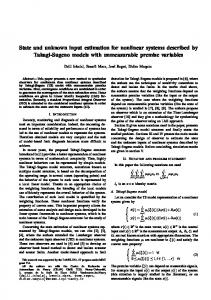
v. Thus, in our wind turbine system, the polytopic representation of LPV model has two subsystems. According to the range of wind speed, the weight of subsystem can be calculated as following vmax −v ρ1 (v) = vmax −vmin , (28) v−vmin ρ2 (v) = vmax −vmin In a wind turbine system, the pitch subsystem starts to work only if the wind speed is up to the rating value. And when the wind speed is over the cut-off wind speed, the pitch subsystem will stop working. In this paper, the variation range of wind speed is chosen in (6, 25), during the pitch subsystem’s working. According to the detail parameters of wind turbine system, the system matrix can be written as a polytopic representation and given as follows     0 1 −0.1031 0 0  −22.39 −0.2196 1.652 × 10−3 −0.00627     , D1 =  0.0249  , A1 =   16744.0 119.84   0  −1.8677 0 0 0 −10.0  0   0  (29) 0 1 −0.1031 0 0  −22.39 −0.7017 1.652 × 10−3 −0.02876     , D2 =  0.0390  A2 =   16744.0 119.84   0  −1.8677 0 0 0 0 0 −10.0 Appling theorem 1 and following the steps, we can obtain the parameters of UIO. The LMIs can be solved by using Yalmip toolbox[22]. The solutions of  matrixes are    0 1.0 −8379.5 0 12569.0 0 −22.344 0.0029615 −5832.9    0 , L1 =  8749.4 0.0041041, N1 =   8372.1   59.922 −2.1612 0 2.3079 −0.00001  0 0 0 −0.67499 0 −3.9875     0 1.0 −8379.5 0 12569.0 0 −22.344 −0.7004 −5832.9   0 −0.028716 , L2 =  8749.4 , N2 =   8372.1  2.3079 59.922 −2.1612 −0.00006 0.00008  0 0 0.00006 −0.67499 −0.00008 −3.9875   0 0 [ ] [ ]  0 0 0.90314 0 1.0 0   G1 = G2 = T =  ,S= . Γ= . 0.31608 0  0 14.287 0 0.002 0 5.0 For the UIO, the wind speed is the main disturbance which is considered as an unknown input vector d(t) (Shown in figure (1)). The initial conditions are considered as the x(0) = [0, 1, 100, 0] and x ˆ(0) = [0, 0, 0, 0]. In this paper, a fault for the pitch actuator system is considered as following { { −0.25u2 (t), 50 ≤ t, 0.3u1 (t), 40 ≤ t, f1 (t) = , f2 (t) = (30) 0, otherwise. 0, otherwise.

7


17

Pitch actuator fault

4

15

2

freal fest

0

−2 0

20

40 Time (s)

60

80

100

14

Rotor actuator fault

Wind speed (m/s)

16

13

12 0

20

40 Time (s)

60

freal

50

f

est

0 −50 −100 −150 0

80

Figure 1. Wind speed

20

40 Time (s)

60

80

Figure 2. Simulation and estimation values of the actuator faults

0.1

θ

θ

10

20

30

40 Time (s)

50

60

70

−0.05

80

Rotor speed( rad/s)

0

2

1

0

ωrreal 0

10

20

30

40 Time (s)

50

ωrest

60

70

80

200

100

0

ωgreal 0

10

20

30

40 Time (s)

50

60

ωgest 70

80

30

0

10

20

30

40 Time (s)

50

60

70

80

0.2

error

ωr

0

−0.2

0

10

20

30

40 Time (s)

50

60

70

80

1

errorωg 0

−1

0

10

20

30

40 Time (s)

50

60

70

80

30

β

β

real

20

Pitch angle

Pitch angle

θ

0

Generator Speed (rad/s)

Generator Speed (rad/s)

Rotor speed( rad/s)

−0.1

error

0.05

est

Theta

Theta

real

0

est

10 0 0

10

20

30

40 Time (s)

50

60

70

10 0 −10

80

errorβ

20

0

10

20

30

40 Time (s)

50

60

70

80

Figure 3. Simulation and estimation values of Figure 4. State errors between simulation and the states estimation The simulation results are illustrated as following. Figure (2) shows the reference and the estimated values of faults . Figure (3) displays the simulated and the estimated values of the system states. From Figure (2), we can see that the estimated value tends to the simulated value rapidly and asymptotically in the absence of fault. The corresponding errors are illustrated in Figure (4). From these results, we can see that the estimation value of the states tend to the simulation value. And the estimation faults change slightly within the scope of the simulation value after the faults occur. It illustrates that the proposed UIO is effective. 5. Conclusions In this paper, an robust UIO is designed for actuator fault diagnosis based on LPV model systems. Considering the disturbance, actuator fault in the wind turbine system, we design and analyze the convergence of the observer using Layapunov and H∞ theory. By solving the LMIs and LMEs, the parameters of theUIO can be found. Computing the residual, the fault signal is generated easily. In addition, a wind turbine system with pitch actuator fault is tested to verify the UIO’s performance. The simulation results show that the proposed method is efficient.

8


Acknowledgments This work is partially supported by the National Natural Science Foundation of China (61304077), by International Science & Technology Cooperation Program of China (2015DFA01710), by the Natural Science Foundation of Jiangsu Province (BK20130765), by the Chinese Ministry of Education Project of Humanities and Social Sciences (13YJCZH171), by the Chinese Ministry of Education Project of Humanities and Social Sciences (13YJCZH171), by the 11th Jiangsu Province Six talent peaks of high level talents project (2014 ZBZZ 005), and by the Jiangsu Province Project Blue: young academic leaders project. This wrok is also supported by Campus France through the Program Partenariats Hubert Curien, Cai Yuanpei. References [1] Szabat K, Tran-Van T, Kami M, x, ski. A Modified Fuzzy Luenberger Observer for a Two-Mass Drive System. IEEE Transactions on Industrial Informatics. 2015, 11, 531-9. [2] Prasov AA, Khalil HK. A Nonlinear High-Gain Observer for Systems With Measurement Noise in a Feedback Control Framework. IEEE Transactions on Automatic Control. 2013, 58, 569-80. [3] Yao J, Jiao Z, Ma D. Extended-State-Observer-Based Output Feedback Nonlinear Robust Control of Hydraulic Systems With Backstepping. IEEE Transactions on Industrial Electronics. 2014, 61, 6285-93. [4] Guan Y, Saif M. A novel approach to the design of unknown input observers. IEEE Transactions on Automatic Control. 1991, 36, 632-5. [5] Hui S, Zak SH. Stress estimation using unknown input observer. 2013 American Control Conference. IEEE2013. p. 259-64. [6] Mondal S, Chakraborty G, Bhattacharyy K. LMI approach to robust unknown input observer design for continuous systems with noise and uncertainties. International Journal of Control, Automation and Systems. 2010, 8, 210-9. [7] Xiong Y, Saif M. Unknown disturbance inputs estimation based on a state functional observer design. Automatica. 2003, 39, 1389-98. [8] Chen W, Saif M. Unknown input observer design for a class of nonlinear systems: an LMI approach. IEEE American Control Conference. 2006, 834-838. [9] Zhang W, Su H, Zhu F, et al. Unknown input observer design for one-sided Lipschitz nonlinear systems. Nonlinear Dynamics, 2015, 79, 1469-1479. [10] Chadli M, Karimi H R. Robust observer design for unknown inputs Takagi-Sugeno models. IEEE Transactions on Fuzzy Systems, 2013, 21,158-164. [11] Kulcsar B, Bokor J, Shinar J. Unknown input reconstruction for LPV systems. International Journal of Robust and Nonlinear Control. 2010, 20, 579-95. [12] Hammouri H, Tmar Z. Unknown input observer for state affine systems: A necessary and sufficient condition. Automatica. 2010, 46, 271-8. [13] Chen J, Patton RJ, Zhang H-Y. Design of unknown input observers and robust fault detection filters. International Journal of Control. 1996, 63, 85-105. [14] Chen W, Saif M. Fault detection and isolation based on novel unknown input observer design. 2006 American Control Conference. IEEE2006. p. 6 pp. [15] Marx B, Koenig D, Ragot J. Design of observers for Takagi-Sugeno descriptor systems with unknown inputs and application to fault diagnosis. IET Control Theory and Applications. 2007, 1, 1487-95. [16] Wang D, Lum KY. Adaptive unknown input observer approach for aircraft actuator fault detection and isolation. International Journal of Adaptive Control and Signal Processing. 2007, 21, 31-48. [17] Hassanabadi AH, Shafiee M, Puig V. UIO design for singular delayed LPV systems with application to actuator fault detection and isolation. International Journal of Systems Science 2016; 47(1): 107-121 [18] Hamdi H, Rodrigues M, Mechmeche C, Theilliol D, Braiek NB. Fault detection and isolation in linear parameter-varying descriptor systems via proportional integral observer. International Journal of Adaptive Control and Signal Processing 2012; 26(3): 224-240. [19] Bianchi FD, De Battista H, Mantz RJ. Wind turbine control systems: principles, modelling and gain scheduling design. Springer Science & Business Media, 2007. [20] Shirazi FA, Grigoriadis KM, Viassolo D. Wind turbine integrated structural and LPV control design for improved closed-loop performance. International Journal of Control 2012; 85(8): 1178-1196. [21] Jonkman JM, Butterfield S, Musial W, Scott G. Definition of a 5-MW reference wind turbine for offshore system development. National Renewable Energy Laboratory Golden, CO, USA, 2009. [22] L¨ ofberg J. YALMIP: A toolbox for modeling and optimization in MATLAB, 2004 IEEE International Symposium on Computer Aided Control Systems Design. IEEE, 2004;284-289.

9