Robustness of Multiple Objective GP Stock-Picking in Unstable Financial Markets Real-World Applications Track Ghada Hassan
Christopher Clack
Department of Computer Science University College London Gower Street, London WC1E 6BT
Department of Computer Science University College London Gower Street, London WC1E 6BT
[email protected]
ABSTRACT Multiple Objective Genetic Programming (MOGP) is a promising stock-picking technique for fund managers, because the Pareto front approximates the risk/reward Efficient Frontier and simplifies the choice of investment model for a given client’s attitude to risk. Unfortunately GP solutions don’t work well if used in an environment that is different from the training environment, and the financial markets are notoriously unstable, often lurching from one market context to another (e.g. “bull” to “bear”). This turns out to be a hard problem — simple dynamic adaptation methods are insufficient and robust behaviour of solutions becomes extremely important. In this paper we provide the first known empirical results on the robustness of MOGP solutions in an unseen environment consisting of real-world financial data. We focus on two well-known mechanisms to determine which leads to the more robust solutions: Mating Restriction, and Diversity Preservation. We introduce novel metrics for Pareto front robustness, and a novel variation on Mating Restriction, both based on phenotypic cluster analysis.
Categories and Subject Descriptors I.2.M [Artificial Intelligence]: Miscellaneous
General Terms Algorithms, Experimentation
Keywords GP, Multiobjective Optimization, Robustness, Portfolio Optimization, Finance, Dynamic Environment
1.
INTRODUCTION
Genetic Programming (GP) is a popular technique for evolving stock-picking models [4, 26, 30, 31]. These mod-
Permission to make digital or hard copies of all or part of this work for personal or classroom use is granted without fee provided that copies are not made or distributed for profit or commercial advantage and that copies bear this notice and the full citation on the first page. To copy otherwise, to republish, to post on servers or to redistribute to lists, requires prior specific permission and/or a fee. GECCO’09, July 8–12, 2009, Montréal Québec, Canada. Copyright 2009 ACM 978-1-60558-325-9/09/07 ...$5.00.
[email protected]
els are equations that combine various time-series inputs to provide a score for a given stock. The manager of an investment portfolio of equities applies a chosen model, buys stocks with a high score and sell stocks with a low score. Because this is low-frequency investment rather than highfrequency trading, the stock-picking model (and thus the buying and selling of stocks) is applied once a month, and the training data consists of time series of monthly data. Multiple Objective GP (MOGP) [5, 16, 20, 21] has an added advantage for a fund manager with many clients, each with a different portfolio and a different appetite for risk. In a bi-objective MOGP using risk and return on investment as the two objectives, the MOGP Pareto front approximates the risk/reward Efficient Frontier [24] and the fund manager can select a suitable model which provides the maximum return on investment for each client’s required risk. Unfortunately, real life is rarely simple, and specifically the financial markets can be extremely unstable. What concerns this research in particular is the correlation between the time series data that is available to the stock-picking model in training and the future performance of a given stock. Our stock-picking models do not have to predict precise future stock prices, but they are required to rank the stocks correctly according to future performance. If the correlation between time series and future stock performance changes, then a given model (equation) may become less effective in ranking stocks. We know from previous work [21, 31] that the performance of these stock-picking equations can vary substantially when used in an environment that is different to the training environment — and that the relative positions of solutions on the Pareto front may switch (which is of concern to a client whose “lowest-risk” portfolio might suddenly become the “highest-risk” portfolio) [16]. So how should the system respond to market instability? One obvious response is to employ dynamic adaptation via retraining, using new training data drawn from the new environments. However, in the context of monthly investment this is problematic: • the most pressing problem is the lack of new data, because the time series comprises only monthly data — it is not feasible to train on just a handful of data points, so the system must wait many months before sufficient new data has been gathered to permit retraining (and by that time, the market may have changed again); • rather than waiting many months, the system may employ a “sliding window” method where it continuously
retrains on the most recent (say) twelve months of data — the disadvantage with this approach is that for the first (say) six months following a change the training data will predominantly come from the old environment, and so it will still take some considerable time before a more suitable equation can be evolved; • how often should the system retrain? too frequently, and too little data will be available: too infrequently, and the retraining may be ineffective because it happens at the wrong time (e.g. just before a change in the market); • should the system only retrain when a change in the market is detected? this would appear to be a better solution, but turns out to be difficult to achieve (see below). Certain gross behaviour of the financial markets (e.g. a “bull”, “bear”, or “volatile” market) can be identified by inspection of the behaviour of a benchmark portfolio (or “index” portfolio) which invests in all stocks equally (alternatively, investing in all stocks using a standard weighting such as capitalisation). The index can therefore be used to identify a change in market environment. However, it turns out to be very difficult to detect the point at which a market changes — it is relatively easy to identify a “bull” or a “bear” market once it is established, but at the turning point it can be difficult to know for certain whether the market is really changing, and difficult to determine the nature of the new market (i.e. is it changing from “bull” to “bear” or from “bull” to “volatile”?). Whilst retraining is an important tool in responding to the instability of the markets it is insufficient on its own; it is also necessary to ensure that the evolved models will continue to perform reasonably well when the market environment in which they are used is different to that in which they were trained. We don’t expect them to continue to behave well but we can require that they degrade gracefully within a range of market change and do not suddenly produce catastrophically wrong results (it would be unreasonable to expect good behaviour for a sudden extreme change). We call this “solution robustness” and it is important because it provides a period of time within which either new data can be gathered for retraining or human intervention can take over prior to retraining. In summary, solution robustness of MOGP is extremely important for the real-world problem of stock-picking for a monthly investment portfolio. It is therefore essential for MOGP solutions to be analysed in unseen environments, not just in training, and although it may be difficult to define an absolute measure of solution robustness we must be able to determine which of two solutions is more robust, and which of two Pareto fronts is more robust.
1.1 Our approach Our investigation focuses on the use of two well-known techniques — Mating Restriction and Diversity Preservation. Following observations of phenotypic clustering in a stock-picking MOGP [15], we hypothesize that each cluster is specializing for a particular niche in the phenotype space rather than fitting to specific data, and therefore restriction of mating to others within the same phenotype cluster may produce more robust individuals. We also know from prior
work that diversity preservation in GP favours smaller trees and therefore avoids over-fitting [3], which we hypothesize will also lead to more robust solutions. Both techniques are known to provide benefits to Multiobjective Evolutionary Algorithms (see Section 2). However, all prior work appears to be restricted to training (e.g. to improve the distribution of solutions on the Pareto front) and we have found no prior work which demonstrates a beneficial effect on the robustness of solutions (nor of the Pareto front) in unseen environments. Specifically, we use SPEA2 [32] to apply an MOGP algorithm to the evolution of factor models for asset selection in a financial portfolio management problem in a dynamic environment. We examine the performance of the evolved solutions on out-of-sample (unseen) environments in comparison to a buy and hold strategy of stocks making up the index (i.e. we compare performance against an index tracker fund). We examine the effect of diversity and a new mating restriction technique based on phenotypic similarity of solutions on the generalisation and robustness of solutions on the out-of-sample environments. We are interested to investigate the following issues: • What are the suitable performance metrics to measure success or failure of solutions in out-of-sample environments (taking into account that a drop in objective values is not a sufficient criterion since the new market conditions may not allow for a higher value)? • Are the trained MOGP solutions suitable for investment in an unseen subsequent environment (how well do they perform in portfolio stock-picking)? • What effect will a special technique of similarity-based mating restriction have on the preservation of each solution’s objective characteristics in unseen environments? The paper is organised as follows. Section two presents related work on MOEA in dynamic environments, previous work on mating restriction in MOEA as well as research on over-fitting avoidance in Genetic Programming. Section three lays the definitions and metrics that will be used throughout the rest of the paper and the proposed mating restriction technique. Section four explains the experimental specifications, followed by results in Section five. Section six concludes.
2. RELATED WORK 2.1 Evolutionary Multiobjective Optimization Evolutionary Multiobjective Optimization (EMO) algorithms [9, 11] are very useful in optimization problems where the decision maker is interested in the knowledge of the various optimal trade-offs that exist between the problem’s objectives. EMO algorithms produce the set of solutions representing this trade-off in a single run. Recent EMO algorithms have been utilised in static training environments to find the optimal trade-off and most research has focused on improving the quality of the solutions, in terms of how close they are to the true Pareto front, and the quality of the front itself in terms of coverage and uniform distribution. Recently, research into optimisation in dynamic multiobjective (DMO) problems has gained a lot of interest [6, 13].
In the dynamic problems studied, the initial training stage has static input data, static constraints and static objective function. Then, a change occurs in one or more aspects of the training environment and the old solution set is no longer optimal. Retraining is usually done to evolve the new Pareto front. During each retraining phase the environment is static and the solutions evolved are to be used in the same static environment until a further change occurs.
2.2 Diversity and Generalisation in GP Diversity maintenance in Evolutionary Computation is essential to prevent premature convergence and improve generalization. Diversity is believed to benefit robustness and generalisation because it favours smaller trees and thereby avoids over-fitting: the work of [29] on generalization of GP used for trading-rule discovery in the foreign exchange market has found that smaller GP trees of depth two or three have led to better generalization in the dollar-yen and dollardm markets. The same result was also found by [1] when evolving technical trading rules for generating buy and sell decisions. Where trees of depth of 2-5 had, on average, outperformed larger trees. It was shown in [3] that changing the balance of crossover and mutation in GP has a significant effect on the generalization capability of the algorithm. Using a mutation rate of 50% yielded the best generalization results, but it decreases if the mutation rate is increased further than the 50%. In addition, the probability of generating an outstanding run also increases by increasing the mutation rate. The beneficial role of mutation was attributed to the decrease in the number of introns. Alternatively, the use of a “selection” set after training is widespread in EA learning in general and was used for GA and GP in the financial domain [2], [8]. However, some researchers [29, 16] have found little gain from the use of a selection set to improve generalization results on the outof-sample set. A detailed study by [7] on selection sets for learning casts a big doubt on their usefulness for avoiding over-fitting; their experimental results suggest that due to the high complexity of the financial data, the addition of a selection set may actually lead to the algorithm becoming less able to exploit the hidden patterns in the data. We are interested to investigate if the generalisation of GP used in the multiobjective frame work will benefit from an increase in mutation rate (and hence diversity) in the same way.
2.3 Mating Restriction in EMO Prior research into the effect of mating restrictions on EMO algorithms has focused mostly on improving quality of the search and/or diversity of the solution set. The effect of mating restriction in the EA literature dates back to [14] who suggested that the crossover between parents who are too different genotypically may hinder the search especially as the population starts to converge. [27] found that restricting the mating to be between a non-dominated individual and another individual that is dominated by it leads to an acceleration (albeit small) in the progress towards the Pareto front. In [12], it was found that recombination between individuals in different niches produces low fitness individuals, and hence a restriction was imposed to prevent mating between dissimilar parents. However, in [19] mating restriction was used to prevent mating between individuals that are too close together in an effort to aid diversity and
help produce a better spread front. In [17], experiments were carried out to examine the effect of mating similar or dissimilar parents on small and large multiobjective test set problems. Again, the results varied: on small test problems, choosing dissimilar parents had improved the search ability; however, on large test problems, the search ability was improved through the choice of similar parents instead. The seemingly contradicting results may be due to (i) the large, complex problems having a large and diverse search space, where the EMO algorithm benefited from the pressure towards convergence through mating of similar parents, whereas (ii) in small problems, convergence to one niche of the Pareto front can happen too soon and the need for improved diversity increases. In summary, the current research on mating restriction in EMO can be divided into two main classes: mating of similar parents or mating of dissimilar parents. The former will speed up convergence and in some problems the quality of the solutions. On the other hand, mating of dissimilar parents will improve diversity, which is vitally important in the EMO search. However, no research was carried out to investigate the effect of encouraging mating of either similar or dissimilar parents on the performance of the EMO on out-of-sample data.
3. MOGP ROBUSTNESS IN DYNAMIC ENVIRONMENTS We are interested in problems with dynamic environments where the environment changes after training. In single objective problems, robustness is dependent on the GP models discovered during training being robust enough such that the underlying relationship is still valid and the fitness remains close enough to the new optimal value. In the case of multiple objectives, more needs to be achieved. First, it is necessary to examine a set of trade-off solutions; the whole of the front is required to be as close as possible to the optimal trade-off surface. In addition, the solutions should maintain their objectives’ cluster classifications as much as possible, such that a solution that was achieving high values on all objectives, will keep the same high classification of objectives in the new environment. Third, we will also be interested in a front which retains its diversity and uniform distribution, so that all regions of the trade-off hyper-surface remain well represented. To develop a metric testing for the degree of preservation of objectives clusters, we used the K-means [23] clustering algorithm to classify the objective values into three clusters in training and then in validation, and compared them. In training, the K-means usually ends up with two clusters on both extremes of all objectives, and one with middle values of all objectives. For example, for a problem with 2 objectives, every solution is classified as belonging to one of the following clusters (see Fig. 1): hHigh, Highi,hMedium, Mediumi,hLow, Lowi A more stringent test for robustness is the preservation of solution rank-order. We used a ranking algorithm that gave ranks to solutions based on sorting the objective values of each objective separately. In training environments the ranking algorithms usually resulted in equivalent ranking for the objective values achieved by each solution, see Fig. 2. For example, if a solution had a rank of (6, 6) then this means that each of its objective values was ranked sixth.
Definition 1 : Objectives Clusters Solutions on the Pareto front are classified into clusters such that members of a cluster have similar classifications for each of their objectives. A cluster Ci is identified by a vector of the m classification values of the cluster centroid (c1 , c2 , ...cm ), where m is the number of objectives. Hence, we have: Cluster(Ci ) = hCluster(o1 ), ..., Cluster(om )i where Cluster(oj ) ∈ {L, M, H} and the j th value in the cluster shows the j th centroid value classification. Figure 1: Classification of solutions into clusters — a robust system is one where solutions do not change clusters as the environment changes
Figure 2: Ranking of solutions — a robust system is one where solutions minimally change their relative rank with respect to other solutions Equal values of objectives ranks was almost always observed in training, but is often not observed in validation. We examined the ranking order of the solutions in validation for how closely correlated they are to their rank order achieved in training. The better the rank order correlation, the more robust the solutions are.
3.1 Definitions and Metrics To quantify robustness in dynamic environments, we need to assess several aspects. • First, are the solutions (presumably near optimal in the training environment) still near optimal in the new environment? From a financial perspective, a relative measure of solution performance can be obtained from a measure of their risk-adjusted return, as given by the Sharpe ratio [28]. • Second, how much have the solutions changed their objectives-cluster and rank-order amongst other solutions on the Pareto front? This provides a degree of confidence that a solution expected to yield a certain relative risk-adjusted-return will have a similar behaviour in the new environment.
Table 1: Cluster Distance Change Measurement High(H) Medium(M) Low(L)
High(H) 0 1 2
Medium(M) 1 0 1
Low(L) 2 l 0
Definition 2: Cluster of a Solution In each generation in training, after the Front has been identified, we run the K-means clustering algorithm which assigns a cluster membership to each solution xk on the front, where k is the index of the solutions, k ∈ [1, n], and n is the total number of solutions on the Pareto front. Thus, for all solutions on the front, the following function is defined: Cluster(xk ) = Ci if xk ∈ Ci To measure cluster change between environments, the clustering algorithm is run again after validation and we measure element-wise differences across the cluster vector and add the differences. For example, in a two-objective problem where only three clusters exist, if a solution moves from a cluster hhigh, highi to hmedium, mediumi then we measure this as a move of length 2, whereas if it moves from hhigh, highi to hlow, lowi then this is given a measure of 4. Table 1 shows the measure for the cluster distance change. Definition 3: Rank of a Solution At the last generation of training, a ranking algorithm is run after the Pareto front has been identified, after which each solution has a rank order and the following function is defined for all solutions on the front: Rank(xk ) = (Ranko1 , Ranko2 , ...Rankom ) where Rankoj is the rank order of objective j value among other objectives values for other solutions on the front. Definition 4: Robustness of a Solution: Robustness of a solution xk to a multiobjective problem is defined qualitatively as the degree of its insensitivity to changes in the environment, and is measured quantitatively by three measures: 1. Is the solution still optimal in the new environment?
• Finally, how good is the spread and distribution of solutions on the new front formed in validation? This can be measured using the same metrics used to measure the distribution characteristics of the front in training.
2. How well it preserved its cluster in the new environment — using the cluster distance change metric ∆k P env1 ∆k = m − (Cluster(oj )env2 ) j=1 (Cluster(oj )
The following definitions and metrics aim to provide understanding and measurement of the second aspect of robustness.
3. How well it preserved its rank-order in the new environment — measured by the rank change metric δk P env1 δk = m − Rank(oj )env2 ) j=1 (Rank(oj )
Definition 5 : Robustness of the Pareto Front : Robustness of the Pareto front between two environments is defined by four measures:
for the simulation of an investment fund with real life constraints and parameters. Finally, the MO algorithm and the GP parameters are presented.
1. How close is the front to the optimal Pareto front?
4.1 Stock Selection for Portfolio Optimization
2. How well its solutions maintain their objectives’ clusters between the two environments — measured by calculating the mean cluster P distance µ across all n solutions in the front: µ = n k=1 (∆(xk )) 3. How well its solutions’ ranks have remained closely correlated between the two environments — measured using a rank correlation test (e.g. Spearman Rank Correlation [25]). The Spearman test returns a number in the range [−1, 1] known as the Spearman Coefficient (ρ). The closer the value is to 1, the stronger the correlation between the two rankings. A value of −1 implies negative correlation and a value of 0 implies independence between the two ranks. n X δk2 ρ(objm ) = 1 − n(n26−1) k=1
4. How well the Pareto front maintained its diversity and uniform distribution — measured using the spacing (S) and hole-relative-size (HRS) metrics [10].1
3.2 Cluster-based Mating Restriction Previous work [15] has shown that solutions evolved for each objectives-cluster have common characteristics that distinguish them from solutions in other clusters. That has led us to believe that in this financial domain, the MOGP is discovering rules belonging to various niches (corresponding to the clusters). If this were actually the case, then by limiting the mating to parents belonging to the same cluster and hence sharing the same objectives characteristics we will further help this speciation. We are interested to investigate the effect this special kind of similarity mating will have on one particular aspect of generalization which is the movement from one cluster to the others between training and validation environments. The MOEA algorithm used is SPEA2 [32], where the underlying evolutionary algorithm is a GP. Individuals in SPEA2 are compared based on Pareto dominance and the non-dominated solutions of each generation are placed in a separate archive. Selection of parents is limited to this archive. We have simulated a mating restriction technique whereby mating is restricted to parents belonging to the same cluster. Parents are selected using binary tournament selection of size 7 with replacement, exactly as in standard SPEA2. The difference is, the second parent is accepted only if it belongs to the same cluster as the first parent. If not, we attempt to reselect the second parent for a maximum of four more times. If we fail to select a parent belonging to the same cluster after five trials, the first parent crosses over with a copy of itself.
4.
EXPERIMENTAL SPECIFICATION
In this section the portfolio optimization problem is described, followed by details of the investment strategy used 1 A Hypervolume metric can also be useful but is not presented here.
An equity portfolio is a collection of stocks, which provides diversification and therefore a degree of protection against the price volatility of underlying individual stocks [24]. The general portfolio optimization problem is the choice of an optimum set of assets to include in the portfolio, and the distribution of investor’s wealth among them, such that the objectives sought by holding the portfolio are maximized. In this work, we are considering two objectives: maximizing the expected portfolio return E and minimizing the portfolio variance V (the average squared deviation of the return P from its expected value). These are given by E = n i=1 xi µi P Pmean n x x σ where n is the number of seand V = n i j ij j=1 i=1 curities in P portfolio, xi is the relative amount invested in security i, n i=1 xi = 1, µi is the mean expected return of security i, and σij is the covariance between assets i and j. These equations are solved by a set of points that constitute the efficient frontier [24] of the problem. The points constituting the curve represent portfolios that give the highest return for a certain expected risk, or the minimum risk for a certain expected return.
4.2 Investment Strategy We simulate a long-only sector-neutral portfolio of 25 stocks. The balanced investment across several industries guards against the price shocks of any one sector. The stocks are selected from the UK stock market as represented by the FTSE100. For every stock, data of 22 financial factors2 over 80 months is available. The total period is divided into training and validation. For training (in-sample), 48 months from May 1999 to April 2003 are used. For validation (outof-sample), the data is that of the last 20 months from May 2004 to December 2005. The return on investment (ROI) of an “Index Fund” portfolio that invests one million pounds, with equal proportions in the 82 stocks of the universe, over the two time periods selected for training and validation, is depicted respectively in Figs. 3 and 4. The investment strategy employed is inspired by real world fund management practices. The portfolio consists of one cash line plus a fixed cardinality of n = 25 stocks. The initial portfolio value is Co = £1, 000, 000 in cash with no stock holdings. After that, the portfolio will constitute of n securities, and the current cash holding will be denoted by C, where we try to keep C less than or equal a maximum bound Cmax = 3% of the total fund value. S is the universe of equities, Sn is the set of securities held in the portfolio. For all buying and selling decisions, it is assumed we can trade at the opening price of that day. During the holding period, interest received on cash holdings is ignored. At the start of each month, we calculate the attractiveness of each stock in S using the factor model (GP decision tree), and rank them accordingly. If any of the stocks we currently hold falls in the bottom quartile, it is sold. If the number of stocks currently in the portfolio is less than n or C > Cmax , then we need to buy stocks from the top quartile, starting with the most attractive. The proportion to be invested in 2 For details of the factors used please refer to [16]. Data supplied by Reuters.
5. EXPERIMENTS AND RESULTS Four sets of simulations were conducted. Results are reported for 15 runs of each system, which are sufficient for the statistical tests that we use to compare all systems against each other - i.e. the Kruskal-Wallis H test and the TukeyKumar test [25]. Statistical results are based on observation of only the unique individuals in the archive to prevent multiples of either good or bad solutions biasing the results. Crossover probability is 0.7 throughout.
5.1 Experiments Four experiments were run as follows. Standard SPEA2 The standard SPEA2 algorithm is used in the simulations. Reproduction probability 0.3, no mutation. Diversity Enhancement Standard SPEA2 with enhanced diversity is used in this set. To increase the diversity, High mutation probability of 0.3, no reproduction. Also, in each generation, after the archive is built, duplicate individuals are deleted.
Figure 3: Index Fund ROI During Training
Mating Restriction The underlying algorithm is SPEA2. However, mating restriction as described in Section 3.2 is employed. For comparison with the first set of simulations, the reproduction probability is 0.3, no mutation. Mating Restriction and Diversity Enhancement Same as the previous set of simulations with the exception that the operators used are crossover with 0.7 probability and mutation with 0.3 probability.
5.2 Results All results reported are regarding the performance of solution on the out-of-sample period.
Figure 4: Index Fund ROI During Validation
each stock is Ci , and is decided by: Ci = min(
C , 4% of total f und value) n − |Sn |
(1)
If cash still exceeds Cmax , it is used to bring each stock holding up to 4% or up to the maximum permitted by the extra cash. Transaction costs of 1.5% of the transaction value are deducted. Additional realistic constraints are imposed: lower and upper bounds on investment per stock, and maximum cash holding.
4.3 Experimental Parameters The multiobjective algorithm used is SPEA2 [32]. The implementation (in Java) is based on the ECJ package [22]. All experiments had a population size of 500, archive size 200, and run for 35 generations, after which no further improvement (in training) was observed regardless of any additional computation. The method of tree generation is ramped half and half [18]. The terminal set for the tree consists of technical and fundamental financial factors describing a company’s performance, plus constants. The function set includes addition, subtraction, multiplication, division, power 2, and power 3. The MOGP has two conflicting objectives to satisfy; return maximization and risk minimization. Return is defined as the annualized average return, and risk is the standard deviation of the annualized average return.
1. Quality of solution - The average quality of solutions was compared for each system (averaged across all solutions in the Front, and across all runs). The Sharpe ratios achieved by using factor models evolved by each of the four techniques for investment during validation show that using diversity-enhanced-mating-restriction gives the best result (Sharpe=2.11), mating restriction comes second (1.95), diversity preservation is third (1.6) and standard SPEA2 has the worst performance (1.42). By comparison, the index performance on the same period (i.e. the performance of an index tracker fund) had a Sharpe ratio of 1.364 — this was measured by simulating a long-only investment of £1, 000, 000 in equal proportion in all 82 stocks making up the index for the duration of the validation period — and the best possible Sharpe ratio achieved was 3.15 (achieved by post-hoc exhaustive training of all systems). 2. Preservation of solutions order - i.e. do solutions retain their relative order on the Front when moving from training to an unseen environment? We use four metrics: the number of solutions that changed cluster, the distance cluster change, the Spearman correlations on both objectives. Fig. 5 shows the number of solutions that changed their cluster as a percentage of the Front size (the smaller the better). Only 31% of the diversity-enhanced-mating-restriction technique have changed their cluster as opposed to 55%
Figure 5: Points Changing Cluster
Figure 8: The HRS and Spread Metrics Table 2: Statistical Test Results (Validation) H P ω
Figure 6: Average Distance Cluster Change in the standard SPEA2. Fig. 6 shows the average distance cluster change (the smaller the better), and Fig. 7 shows the Spearman coefficient (the closer to 1 the better)for objectives one (Rho1) and objective two (Rho2). 3. Distribution of solutions on the front - Measured using the spread and HRS metrics, where on both metrics smaller values are better. Fig. 8 shows the average values achieved for the two metrics respectively. On the spread metric, standard SPEA2 achieved the worst, and MR+DIV achieved the best, average value. However, on the HRS metric, the SPEA2 had the best value, and mating restriction the worst. The results of the Kruskal-Wallis statistical analysis are given by H and P in Table 2 — the final row indicates the value of ω from a Tukey-Kumar test. For example: the Sharpe Ratio’s ω value of 0.44 indicates that any two systems with Sharpe Ratio means differing by at least 0.44 are drawn from different populations with a significance given by the P-value (in this case 94%). These results indicate
Figure 7: Spearman Correlation Coefficient
Avg Dist Change 5.817 0.121 11.44
% Change 3.958 0.266 0.29
RHO1 1.723 0.632 0.16
RHO2 6.964 0.073 0.225
Sharpe 7.512 0.057 0.44
that SPEA2 and MR+DIV differ significantly in both the Sharpe Ratio (94%) and RHO2 (93%).
6. CONCLUSION We have applied an MOGP algorithm to the evolution of factor models for stock selection in a financial portfolio management problem. The evolved factor models represent investment models of an underlying relationship between the financial factors considered. Due to the dynamic nature of the financial market, the optimal values of its efficient frontier are continuously changing. If these algorithms are to be judged useful in such a real world environment, the factor models evolved in the training phase must be robust in subsequent environments — they must remain reasonably profitable (at reasonable risk) for long enough to permit new data to be gathered for retraining. We have investigated the performance of evolved MOGP solutions using SPEA2 in an unseen, out-of-sample environment. A mating restriction scheme based on phenotype clusters was developed to improve robustness, and compared with both the standard SPEA2 system and SPEA2 with additional mutation (to improve population diversity). Results indicate that diversity in MOGP generalization plays a role similar to that played in GP, and further investigation of the effect of various levels of mutation and other diversity enhancement techniques on generalization in MOGP should be worthwhile. We have found that the introduction of cluster-based mating restriction in addition to the increase in diversity provided the best generalization results while also greatly enhancing the quality of solutions as measured by the Sharpe ratio. This result supports the hypothesis that speciation occurs in MOGP and that preserving the niche characteristics can benefit robustness. Results in this research are entirely based on empirical evaluation in the field of evolving stock selection rules for monthly investment and statistical analysis of the results. Our insights from the field and from previous related research back up the results found. However more theoretical analysis is needed to improve the understanding of factors
that affect the generalization of multiobjective evolutionary algorithms and hence improve their usability as optimization tools in financial and other complex real world problems. For further future work, we would like to expand this study to include training and validation of the MOGP in a variety of financial environments. Also of great interest is to investigate a suitable measure for the severity of change in the financial context, and consequently account for the maximum change to which an MOGP solution is robust.
7.
REFERENCES
[1] L. B. L. A. and M. Seshadri. GP–evolved technical rules can outperform buy and hold. Proc.6th Int’l Conf. on Computational Intelligence and Natural Computing, pages 26–30, 2003. [2] F. Allen and R. Karjalainen. Using genetic algorithms to find technical trading rules. Journal of Financial Economics, 51:245–271, 1999. [3] W. Banzhaf, F. D. Francone, and P. Nordin. The effect of extensive use of the mutation operator on generalization in genetic programming using sparse data sets. In PPSN IV, Proc. EC’96. [4] Y. Becker, P. Fei, and A. M. Lester. Stock selection : An innovative application of genetic programming methodology. In GPTP IV. [5] Y. L. Becker, H. Fox, and P. Fei. An empirical study of multi-objective algorithms for stock ranking. In GPTP V. [6] L. T. Bui, J. Branke, and H. A. Abbass. Multi-objective optimization for dynamic environments. Proc. CEC’05. [7] S.-H. Chen and T.-W. Kuo. ”over fitting or poor learning: A critique of current financial applications. EuroGP 2003, pages 34–46, 2003. [8] P. W. Christopher Neely and R. Dittmar. Is technical analysis in the foreign exchange market profitable? a genetic programming approach. Journal of Financial and Quantitative Analysis, 4(32):405–426, 1997. [9] C. A. Coello. Recent trends in evolutionary multiobjective optimization. In Evolutionary Multiobjective Optimization: Theoretical Advances and Applications, pages pp. 7–32. Springer–Verlag, 2005. [10] Y. Collette and P. Siarry. Multiobjective Optimization: Principles and Case Studies. Springer, 2003. [11] K. Deb. Multi–Objective Optimization using Evolutionary Algorithms. John Wiley and Sons, 2001. [12] K. Deb and D. E. Goldberg. An investigation of niche and species formation in genetic function optimization. In Proc. GA’89. [13] K. Deb, U. B. R. N., and S. Karthik. Dynamic multi-objective optimization and decision-making using modified NSGA-II: A case study on hydro-thermal power scheduling. In EMO, pages 803–817, 2006. [14] D. E. Goldberg. Genetic Algorithms in Search, Optimization, and Machine Learning. Addison–Wesley, 1989. [15] G. Hassan. Non–linear factor model for asset selection using multi objective genetic programming. In GECCO–2008 Workshop: Advanced Research Challenges in Financial Evolutionary Computing (ARC–FEC), pages 1859–1862. ACM, 2008.
[16] G. Hassan and C. D. Clack. Multiobjective robustness for portfolio optimization in volatile environments. In Proc. GECCO ’08, pages 1507–1514. ACM, 2008. [17] H. Ishibuchi and Y. Shibata. An empirical study on the effect of mating restriction on the search ability of EMO algorithms. LNCS, pages 433–447, 2003. [18] J. R. Koza. Genetic Programming: On the Programming of Computers by Means of Natural Selection. MIT Press ,Cambridge, MA, USA, 1992. [19] R. Kumar and P. Rockett. Improved sampling of the pareto-front in multiobjective genetic optimizations by steady-state evolution: A pareto converging genetic algorithm. Evolutionary Computation, 10(3):283–314, 2002. [20] D. Laura. A multi–objective evolutionary approach to the portfolio optimization problem. International Conference on Computational Intelligence for Modelling, Control, and Automation, 2005. [21] J. Li and S. Taiwo. Enhancing financial decision making using multi–objective financial genetic programming. Proceedings of IEEE Congress on Evolutionary Computation, pages 7935–7942, 2006. [22] S. Luke et al. A java–based evolutionary computation research system, version 15. http://www.cs.gmu.edu/ eclab/projects/ecj/. [23] J. MacQueen. Some methods for classification and analysis of multivariate observations. In Proceedings of the 5th Berkeley Symposium on Mathematical Statistics and Probability, pages 281–297. UC Press, Berkeley, CA, USA, 1967. [24] H. Markowitz. Portfolio selection. Journal of Finance, 7(1):77–91, 1952. [25] W. Mendenhall, R. Beaver, and B. Beaver. Introduction to Probability and Statistics. Duxbury Press, 1999. [26] J.-Y. Potvin, P. Soriano, and M. Vallee. Generating trading rules on the stock markets with genetic programming. Computers & Operations Research, 31(7):1033–1047, 2004. [27] O. Roudenko and M. Schoenauer. Dominance based crossover operator for evolutionary multi-objective algorithms. LNCS, 3242:812–821, 2004. [28] W. F. Sharpe. Capital asset prices: A theory of market equilibrium under conditions of risk. Journal of Finance, 19(3):425–442, 1964. [29] J. D. Thomas and K. Sycara. The importance of simplicity and validation in genetic programming for data mining in financial data. In Data Mining with Evolutionary Algorithms: Research Directions, pages 7–11, 1999. [30] W. Yan and C. D. Clack. Behavioral GP diversity for dynamic environments: an application in hedge fund investment. Proc. GECCO’06. [31] W. Yan and C. D. Clack. Evolving robust GP solutions for hedge fund stock selection in emerging markets. In Proc. GECCO ’07. [32] E. Zitzler, M. Laumanns, and L. Thiele. SPEA2: Improving the strength Pareto evolutionary algorithm for multiobjective optimization. Evolutionary Methods for Design, Optimization, and Control, CIMNE, pages 95–100, 2002.