Role of dimensionality in complex networks: Connection with nonextensive statistics S.G.A. Brito1 ,∗ L.R. da Silva1,2 ,† and Constantino Tsallis2,3‡
arXiv:1509.07141v1 [cond-mat.stat-mech] 23 Sep 2015
1 Departamento de F´ısica Te´ orica e Experimental, Universidade Federal do Rio Grande do Norte, Natal, RN, 59078-900, Brazil 2 National Institute of Science and Technology of Complex Systems, Brazil and 3 Centro Brasileiro de Pesquisas Fisicas, Rua Xavier Sigaud 150, 22290-180 Rio de Janeiro-RJ, Brazil and Santa Fe Institute, 1399 Hyde Park Road, New Mexico 87501, USA
Deep connections are known to exist between scale-free networks and non-Gibbsian statistics. For −k/κ , example, typical degree distributions at the thermodynamical limit are of the form P (k) ∝ eq 1 z where the q-exponential form eq ≡ [1 + (1 − q)z] 1−q optimizes the nonadditive entropy Sq (which, for q → 1, recovers the Boltzmann-Gibbs entropy). We introduce and study here d-dimensional geographically-located networks which grow with preferential attachment involving Euclidean dis−αA tances through rij (αA ≥ 0). Revealing the connection with q-statistics, we numerically verify (for d =1, 2, 3 and 4) that the q-exponential degree distributions exhibit, for both q and κ, universal dependences on the ratio αA /d. Moreover, the q = 1 limit is rapidly achieved by increasing αA /d to infinity. PACS numbers: 89.75.Hc, 05.70.-a, 05.45.Pq, 89.75.Da
Networks emerge spontaneously in many natural, artificial and social systems. Their study is potentially important for physics, biology, economics, social sciences, among other areas. For example, many empirical studies have identified peculiar properties in very different networks such as the Internet and online social networks (e.g., Facebook), citations networks, neurons networks [1–3], to quote but a few. An ubiquitous class of such networks is constituted by the scale-free ones (more precisely, asymptotically scale-free). As we shall soon verify, these networks can be seen as a particular application of nonextensive statistical P mechanics, based on 1− i pqi the nonadditive entropy Sq = k q−1 (q ∈ R; S1 = P SBG≡ − k i pi ln pi , where BG stands for BoltzmannGibbs) [4, 5]. This current generalization of the BG entropy and corresponding statistical mechanics has been widely successful in clarifying the foundations of thermal statistics as well as for applications in complex systems in high-energy collisions at LHC/CERN (CMS, ALICE, ATLAS and LHCb detectors) and at RHIC/Brookhaven (PHENIX detector) [6], cold atoms [7], dusty plasmas [8], spin-glasses [9], trapped ions [10], astrophysical plasma [11], biological systems [12], type-II superconductors [13], granular matter [14] (see [15]). The deep relationship between scale-free networks and q-statistics started being explored in 2005 [16–18], and is presently very active [19–23]. The basic connection comes (along the lines of the BG canonical ensemble) from the fact that, if we optimize the funcR 1− dk[P (k)]q with the constraint tional Sq [P (k)] = k q−1 R hki ≡ dk kP (k) = constant or analogous (k being the degree of a generic site, i.e., the number of links
∗ † ‡
E-mail address:
[email protected] E-mail address:
[email protected] E-mail address:
[email protected]
that arrive to a given site; P (k) denotes the degree or connectivity distribution), we straightforwardly obtain 1 −k/κ P (k) = P (0)eq = P (0)/[1 + (q − 1)k/κ] q−1 , which turns out to be the generic degree distribution for virtually all kinds of scale-free networks. The q-exponential 1 function is defined as ezq ≡ [1 + (1 − q)z] 1−q (ez1 = ez ). We verify that, for q > 1 and k → ∞, P (k) ∼ 1/k γ with γ ≡ 1/(q − 1). The classical result γ = 3 [24] corresponds to q = 4/3. In the present work we address the question of how universal such results might be, and more specifically, how P (k) varies with the dimension d of the system? Our growing model starts with one site at the origin. We then stochastically locate a second site (and then a third, a fourth, and so on up to N ) through the ddimensional isotropic distribution p(r) ∝
1 rd+αG
(αG > 0; d = 1, 2, 3, 4) ,
(1)
where r ≥ 1 is the Euclidean distance from the newly arrived site to the center of mass of the pre-existing system (in one dimension, r = |x|; in two p dimensions, r = p x2 + y 2 ; in three dimensions r = x2 + y 2 + z 2 , and so on); p(r) is zero for 0 ≤ r < 1; the subindex G stands for growth. We consider αG > 0R so that the distribu∞ tion P (r) is normalizable; indeed, 1 dr rd−1 r−(d+αG ) = R∞ 1+αG , which is finite for αG > 0, and diverges 1 dr 1/r otherwise. See Fig.1. Every new site which arrives is then attached to one and only one site of the pre-existing cluster. The choice of the site to be linked with is done through the following preferential attachment probability: ki rij −αA Πij = P ∈ [0, 1] (αA ≥ 0) , ki rij −αA
(2)
where ki is the connectivity of the i-th pre-existing site (i.e., the number of sites that are already attached to site
2 i), and rij is the Euclidean distance from site i to the newly arrived site j; subindex A stands for attachment. For αA approaching zero and arbitrary d, the physical distances gradually loose relevance and, at the limit αA = 0, all distances becomes irrelevant in what concerns the connectivity distribution, and we therefore recover the Barab´ asi-Albert (BA) model [24], which has topology but no metrics. 1
30
d =1
15 0
y
y
0
d =2
−15 −1 −60 −40 −20
0
20
x
40
−30 −30
60
−15
0
15
x
30
d =3 30 15 0z −15
−30
−15
x0
−30 30 15 0y −15 15 30−30
FIG. 1. Distribution of N = 500 sites obtained with Eq. (1) for αA = 2.0, αG = 0.0, and d = 1, 2, 3.
10
P ( k)
10
10
10
0
αG αG αG αG αG αG
-2
-4
=0.0 =1.0 =2.0 =3.0 =4.0 =5.0
P ( k)
10
10
=0.0 =1.0 =2.0 =3.0 =4.0 =5.0
0
αG αG αG αG αG αG
-2
-4
=0.0 =1.0 =2.0 =3.0 =4.0 =5.0
κ ≃ 4.90 − 3.45 q .
-6
d =3 10
αG αG αG αG αG αG
d =2
-8
10
10
=0.0 =1.0 =2.0 =3.0 =4.0 =5.0
-6
d =1 10
αG αG αG αG αG αG
d =4
-8
10
0
10
1
10
2
k
10
3
4
10 10
0
10
1
10
2
k
10
3
10
(d = 1, 2, 3, 4) models for fixed (αG , αA ), and we have verified in all cases that the degree distribution P (k) is completely independent from αG : see Fig. 2. Using this fact, we have arbitrarily fixed αG = 2, and have numerically studied the influence of (d, αA ) on P (k): see Figs. 3 and 4. In all cases, the q-exponential fittings −k/κ P (k) = P (0)eq with q > 1 and κ > 0 have been remarkably good. The best fitting values for (q, κ) are indicated in Fig. 5. From normalization of P (k), P (0) can be expressed as a straightforward function of (q, κ). Our most remarkable results are presented in Fig. 6, namely the fact that both the index q and the characteristic degree (or “effective temperature”) κ do not depend from (αA , d) in an independent manner but only from the ratio αA /d. This nontrivial fact puts the growing d-dimensional geographically located models that have been introduced here for scale-free networks, on similar footing as long-range-interacting many-body classical Hamiltonian systems such as the inertial XY planar rotators [25] (possibly the generic inertial n-vector rotators as well [26]) and Fermi-Pasta-Ulam [27] oscillators, assuming that the strength of the two-body interaction decreases with distance as 1/(distance)α . Moreover, as first pointed out generically by Gibbs himself [28], we have the facts that the BG canonical partition function of these classical systems anomalously diverges with size for 0 ≤ α/d ≤ 1 (long-range interactions, e.g., gravitational and dipole-monopole interactions) and converges for α/d > 1 (short-range interactions, e.g., LennardJones interaction), and the internal energy per particle is, in the thermodynamical limit, constant for short-range interactions whereas it diverges like N 1−α/d for longrange interactions, N being the total number of particles. If all these meaningful scalings are put together, we obtain a highly plausible scenario for the respective domains of validity of the Boltzmann-Gibbs (additive) entropy and associated statistical mechanics, and that of the nonadditive entropies Sq (with q 6= 1) and associated statistical mechanics. Finally, we notice in Fig. 6 that both q and κ approach quickly their BG limits (q = 1) for αA /d → ∞. Moreover, the same exponential e1−α/d appears in both heuristic expressions for q and κ. Consequently, the following linear relation can be straightforwardly established:
4
FIG. 2. Connectivity distribution for d = 1, 2, 3, 4, αA = 2.0 and typical values for αG . The simulations have been run for 103 samples of N = 105 sites each. We verify that P (k) independs from αG (∀d).
Large-scale simulations have been performed for the
(3)
In fact, this simple relation is numerically quite well satisfied as can be seen in Fig. 7. Its existence reveals an interesting peculiarity of the nature of q-statistics. If in the celebrated BG factor e−energy/kT , corresponding to q = 1, we are free to consider an arbitrary value for T , how come in the present problem, κ is not a free parameter but has instead a fixed value for each specific model that we are focusing on? This is precisely what occurs in the high-energy applications of q-statistics, e.g., in quarkgluon soup [29] where q = 1.114 and T = 135.2 M ev, as well as in all the LHC/CERN and RHIC/Brookhaven experiments [6]. Another example which is reminiscent
3 10
10
0
αA =0.0
10
10
10
-4
10
0
=0.0 =3.0 =4.0 =5.0 P(0)eq −κ/k
-4
10
=0.0 =3.0 =4.0 =5.0 P(0)eq −κ/k
αA αA αA αA
-2
P ( k)
P(k)
d =2
αA =8.0 -2
αA αA αA αA
-4
-6
10
d =3
-6
d =4
-8
10
0
10
1
10
2
k
10
3
4
10 10
0
10
1
10
2
k
10
3
4
10 10
0
10
1
10
2
k
10
3
10
4
ACKNOWLEDGMENTS
We have benefitted from fruitful discussions with D. Bagchi, E.M.F. Curado, F.D. Nobre, P. Rapcan and G. Sicuro. We gratefully acknowledge partial financial support from CNPq and Faperj (Brazilian agencies) and from the John Templeton Foundation-USA.
[1] S.H. Strogatz, Nature 410 (6825), 268 (2001). [2] M.E.J. Newman, SIAM Review 45 (2), 167 (2003). [3] L. da Fontoura Costa, O.N. Oliveira Jr., G. Travieso, F.A. Rodrigues, P.R.V. Boas, L. Antiqueira, M.P. Viana, L.E.C. Rocha, Advances in Physics 60 (3), 329 (2011). [4] C. Tsallis, J. Stat. Phys. 52, 479 (1988) [First appeared in 1987 as preprint CBPF-NF-062/87, ISSN 0029-3865, Centro Brasileiro de Pesquisas Fisicas, Rio de Janeiro]. [5] M. Gell-Mann, C. Tsallis, eds., Nonextensive entropy Interdisciplinary applications, (Oxford University Press, New York, 2004); C. Tsallis, Introduction to nonexten-
10
1
10
2
3
10 10
0
10
1
10
αA αA αA αA αA
−20 −40
10
3
. . . = 2.0 = 3.0 =0 0 =1 0 =1 5
q = 1.333 q = 1.305 q = 1.200 q = 1.125 q = 1.059
αA αA αA αA αA
=2 5
. . . = 3.0 = 5.0
q = 1.333 q = 1.305 q = 1.235 q = 1.184 q = 1.090
. . . = 6.0 = 8.0
q = 1.333 q = 1.324 q = 1.273 q = 1.210 q = 1.140
=0 0 =2 0
−60 −80
d =1
d =2
−100 0
αA αA αA αA αA
−20
P(k)/P(0)]
2
k
0
lnq [
of this type of behavior is the sensitivity to the initial conditions at the edge of chaos (Feigenbaum point) of the logistic map; indeed, the inverse q-generalized Lyapunov exponent satisfies the linear relation 1/λq = 1 − q [30]. The cause of this interesting and ubiquitous feature comes from the fact that q-statistics typically emerges at critical-like regimes and is deeply related to an hierarchical occupation of phase space (or Hilbert space or Fock space), which in turn points towards asymptotic power-laws (see also [31]). In other words, κ plays a role analogous to a critical temperature, which is of course not a free parameter but is instead fixed by the specific model.
0
k
lnq [
FIG. 3. Degree distribution for d = 1 (blue diamonds), 2 (green triangles), 3 (magenta squares), 4 (grey circles), and typical values of αA , with αG = 2.0. The simulations have been run for 103 samples of N = 105 sites each.
10
P(k)/P(0)]
10
d =1
-6
10
αA =6.0
10
10
-4
0
αA =5.0
10
-2
-8
10
10
=0.0 =3.0 =4.0 =5.0 P(0)eq −κ/k αA αA αA αA
-6
10 10
=0.0 =3.0 =4.0 =5.0 P(0)eq −κ/k αA αA αA αA
αA =3.0
-2
P(k)
P ( k)
10
αA =2.0
0
−40
. . . = 4.0 = 5.0 =0 0 =3 0 =3 5
q = 1.333 q = 1.315 q = 1.270 q = 1.215 q = 1.158
αA αA αA αA αA
=0 0 =4 0 =5 0
−60 −80 −100 0
d =3 20
d =4 40
k
60
80
100 0
20
40
k
60
80
100
FIG. 4. Fittings of the d = 1, 2, 3, 4 connectivity distributions with the function P (k) = P (0)eq −κ/k , where ezq ≡ [1 + (1 − q)z]1/(1−q) . The data are those of Fig. 3. Top: log-log representation. Bottom: lnq [P (k)/P (0)] versus k representation. The fitting parameters are exhibited in Fig. 5. The numerical failure, at large enough values of k, with regard to straight lines are finite-size effects that gradually disappear when we approach the thermodynamic limit N → ∞.
sive statistical mechanics - Approaching a complex world, (Springer, New York, 2009). [6] CMS Collaboration, Phys. Rev. Lett. 105, 1 (2010), and J. High Energy Phys. 8, 86 (2011); ALICE Collaboration, Phys. Lett. B 693, 53 (2010), and Phys. Rev. D 86, 112007 (2012); ATLAS Collaboration, New J. Phys. 13, 053033 (2011); PHENIX Collaboration, Phys. Rev. D 83, 052004 (2011), and Phys. Rev. C 84, 044902 (2011); C.Y. Wong and G. Wilk, Phys. Rev. D 87, 114007 (2013); L. Marques, E. Andrade-II and A. Deppman, Phys. Rev. D 87, 114022 (2013); LHCb Collaboration, CERN-PH-EP-
4 1.4
1.4
d =1 d =2 d =3 d =4
1.3
1.3 BA
4 3 q (αA/d) = 1 1− αA e d +1 3
1.2
0 ≤ αA/d ≤ 1
if
αA/d > 1
q
q
1.2
if
1.1
1.1
1.0
0
d=1 d=2 d=3 d=4
1.0 1
2
3
4
αA
5
6
7
8
9
0
1
2
4
3
5
6
7
8
9
αA/d
1.4
d=1 d=2 d=3 d=4
1.4 1.2 1.0
κ
κ
1.0 0.6
d =1 d =2 d =3 d =4
0.2
0
1
2
3
4
αA
5
6
7
8
0.8
κ (αA/d) =
0.3
αA
−1.15e1− d + 1.45
if
0 ≤ αA/d ≤ 1
if
αA/d > 1
0.6 0.4 9
0.2 0
1
2
3
4
5
6
7
8
9
αA/d
2015-223, LHCb-PAPER-2015-032, 1509.00292 [hep-ex]. [7] P. Douglas, S. Bergamini, and F. Renzoni, Phys. Rev. Lett. 96, 110601 (2006). [8] B. Liu and J. Goree, Phys. Rev. Lett. 100, 055003 (2008). [9] R.M. Pickup, R. Cywinski, C. Pappas, B. Farago, and P Fouquet, Phys. Rev. Lett 102, 097202 (2009). [10] R.G. DeVoe, Phys. Rev. Lett. 102, 063001 (2009). [11] L.F. Burlaga, A.F. Vinas, N.F. Ness, and M.H. Acuna, Astrophys J. 644, L83 (2006); G. Livadiotis and D.J. McComas, Astrophys. J. 741, 88 (2011). [12] A. Upadhyaya, J.-P. Rieu, J.A. Glazier and Y. Sawada, Physica A 293, 549 (2001). [13] J.S. Andrade, Jr, G.F.T da Silva, A.A. Moreira, F.D. Nobre and E.M.F. Curado, Phys. Rev. Lett 105, 260601 (2010). [14] G. Combe, V. Richefeu, M. Stasiak and A.P.F. Atman, Experimental validation of nonextensive scaling law in confined granular media, arxiv 1507.07268. [15] For a regularly updated bibliography see http://tsallis.cat.cbpf.br/biblio.htm [16] D.J.B. Soares, C. Tsallis, A.M. Mariz and L.R. da Silva, EPL 70 (1), 70 (2005). [17] S. Thurner and C. Tsallis, EPL 72, 197 (2005). [18] S. Thurner, Europhysics News 36 (6), 218 (2005). [19] J.S. Andrade Jr., H.J. Herrmann, R.F. Andrade and L.R. da Silva, Phys. Rev. Lett. 94, 018702 (2005). [20] P.G. Lind, L.R. da Silva, J.S. Andrade Jr. and H.J. Herrmann, Phys. Rev. E 76, 036117 (2007).
FIG. 6. q and κ versus αA /d (same data as in Fig. 5). We see that q = 4/3 for 0 ≤ αA /d ≤ 1, and a nearly exponential behavior emerges for αA /d > 1 (∀d); similarly for κ. These results exhibit the universality of both q and κ. The red dot indicates the Barab´ asi-Albert (BA) universality class q = 4/3 [24].
d =1 d =2 d =3 d =4
1.4
1.2
1.0
κ
FIG. 5. q and κ for d = 1, 2, 3, 4. For αA = 0 and ∀d, we recover the Barab´ asi-Albert universality class q = 4/3 (hence γ = 3) [24], which has no metrics.
0.8
0.6
0.4
0.2 1.00
1.05
1.10
1.15
1.20
q
1.25
1.30
1.35
FIG. 7. All the values of q and κ for the present d = 1, 2, 3, 4 models follow closely the linear relation Eq. (3) (continuous straight line). The upmost value of q is 4/3, yielding κ ≃ 0.3 (∀d).
[21] G.A. Mendes, L.R. da Silva and H.J. Herrmann, Physica A 391, 362 (2012).
5 [22] M.L. Almeida, G.A. Mendes, G.M. Viswanathan and L.R. da Silva, European Phys. J. B 86, 38 (2013). [23] A. Macedo-Filho, D.A. Moreira, R. Silva and L.R. da Silva, Phys. Lett. A 377, 842 (2013). [24] A. L. Barab´ asi and R. Albert, Science 286, 509 (1999). [25] C.M. Antoni and S. Ruffo, Phys. Rev. E 52, 2361 (1995); C. Anteneodo and C. Tsallis, Phys. Rev. Lett. 80, 5313 (1998); A. Campa, A. Giansanti, D. Moroni, C. Tsallis, Phys. Lett. A 286, 251(2001); L.J.L. Cirto, V.R.V. Assis and C. Tsallis, Physica A 393, 286-296 (2014). [26] F.D. Nobre and C. Tsallis, Phys. Rev. E 68, 036115 (2003); L.J.L. Cirto, L.S. Lima and F.D. Nobre, J. Stat. Mech. P04012 (2015). [27] H. Christodoulidi, C. Tsallis and T. Bountis, EPL 108, 40006 (2014); D. Bagchi and C. Tsallis, Sensitivity to initial conditions of d-dimensional long-rangeinteracting Fermi-Pasta-Ulam model: Universal scaling, arxiv 1509.04697. [28] J.W. Gibbs, Elementary Principles in Statistical Mechanics – Developed with Especial Reference to the Rational Foundation of Thermodynamics (C. Scribner’s Sons, New York, 1902; Yale University Press, New Haven, 1948); OX Bow Press, Woodbridge, Connecticut, 1981).
In his words: “In treating of the canonical distribution, we shall always suppose the multiple integral in equation (92) [the partition function, as we call it nowadays] to have a finite value, as otherwise the coefficient of probability vanishes, and the law of distribution becomes illusory. This will exclude certain cases, but not such apparently, as will affect the value of our results with respect to their bearing on thermodynamics. It will exclude, for instance, cases in which the system or parts of it can be distributed in unlimited space [...]. It also excludes many cases in which the energy can decrease without limit, as when the system contains material points which attract one another inversely as the squares of their distances. [...]. For the purposes of a general discussion, it is sufficient to call attention to the assumption implicitly involved in the formula (92).” [29] D.B. Walton and J. Rafelski, Phys. Rev. Lett. 84, 31 (2000). [30] M.L. Lyra and C. Tsallis, Phys. Rev. Lett. 80, 53 (1998); F. Baldovin and A. Robledo, Phys. Rev. E 69, 045202(R) (2004). [31] A. Plastino, E.M.F. Curado and F.D. Nobre, Physica A 403, 13 (2014).