RAPID COMMUNICATIONS
PHYSICAL REVIEW E 82, 030102共R兲 共2010兲
Role of infinite invariant measure in deterministic subdiffusion Takuma Akimoto1,* and Tomoshige Miyaguchi2
1
Department of Mechanical Engineering, Keio University, Yokohama 223-8522, Japan Department of Applied Physics, Graduate School of Engineering, Osaka City University, Osaka 558-8585, Japan 共Received 11 May 2010; revised manuscript received 31 July 2010; published 7 September 2010兲
2
Statistical properties of the transport coefficient for deterministic subdiffusion are investigated from the viewpoint of infinite ergodic theory. We find that the averaged diffusion coefficient is characterized by the infinite invariant measure of the reduced map. We also show that when the time difference is much smaller than the total observation time, the time-averaged mean square displacement depends linearly on the time difference. Furthermore, the diffusion coefficient becomes a random variable and its limit distribution is characterized by the universal law called the Mittag-Leffler distribution. DOI: 10.1103/PhysRevE.82.030102
PACS number共s兲: 05.40.Fb, 05.45.Ac, 87.15.Vv
Anomalous subdiffusion, where the mean squared displacement 共MSD兲 is 具x2共t兲典 ⬀ t␣ 共0 ⬍ ␣ ⬍ 1兲, is a ubiquitous feature of nonequilibrium phenomena. Subdiffusion has been observed in various types of experiments: charge-carrier transport in amorphous semiconductors 关1兴, Brownian motion of polymers 关2兴, chain diffusion in polymer melts 关3兴, aftershock diffusion in earthquakes 关4兴, and diffusion in cells and membranes 关5–9兴. In particular, subdiffusion in singleparticle trajectories has recently attracted significant interest from the biological community because of the progress in single molecule experiments 关5–9兴. There are roughly three types of mechanisms that generate subdiffusion: 共i兲 anti-persistence 共e.g., the fractional Brownian equation兲, 共ii兲 geometric disorder 共e.g., diffusion within fractal objects such as percolation clusters兲, and 共iii兲 long-time trappings characterized by a power law 关e.g., nonhyperbolic dynamical systems and continuous time random walks 共CTRWs兲兴. Although the time-averaged MSD 共TAMSD兲 equates to the ensemble-averaged MSD 共EAMSD兲 for 共i兲 and 共ii兲, it is not true for 共iii兲 关10–12兴. Thus, for case 共iii兲, the usual ergodicity, i.e., “the time average 共TA兲 coinciding with the ensemble average 共EA兲,” is violated. However, a generalization of the usual ergodicity would be valid 共i.e., ergodicity in an infinite measure space 关13兴兲; it states that the normalized TA coincides with EA ⫻ Y 关see Eq. 共5兲兴, where Y is a random variable with a universal distribution 共the Mittag-Leffler distribution兲. This distributional behavior is reminiscent of the random behavior of the diffusion coefficient in cells 关6–9兴. EAMSD is defined as K
1 k − xk0兲2 , 具共xm − x0兲 典E ⬅ lim 兺 共xm K→⬁ K k=1 2
共1兲
N−1
1 具共xm − x0兲 典T共N兲 ⬅ 兺 共xk+m − xk兲2 . N k=0 2
共2兲
For CTRW, it has been shown that TAMSD grows linearly in time 关10,15兴: 具共xm − x0兲2典T共N兲 = Dm
共m Ⰶ N兲,
共3兲
and that the diffusion coefficients D are random variables 关10兴. Additionally, the following scaling in terms of N has been theoretically demonstrated 关10,12,15兴, 具具共xm − x0兲2典T共N兲典E ⬀ N␣−1 ,
共4兲
where 具 · 典E represents the ensemble average with respect to initial points and ␣ is the exponent in subdiffusion, 具共xm − x0兲2典E ⬀ m␣. Moreover, TAMSD for the fixed time difference m has been shown to obey the Mittag-Leffler distribution 关15兴. In this Rapid Communication, we study deterministic subdiffusions generated by intermittent maps from infinite ergodic theory. Our main result is that the diffusion coefficient of TAMSD is characterized by the infinite invariant measure of the reduced map. We also show analytically that the distribution function of the diffusion coefficient converges to the Mittag-Leffler distribution and that TAMSD increases linearly in time m without taking the ensemble average. Reviews of infinite ergodic theory. We give a brief review here of infinite ergodic theory. Let T be a conservative 关16兴, ergodic 关17兴, measure preserving transformation on a phase space I and let be an invariant measure. Darling-KacAaronson theorem 共DKA theorem兲 关13,18,19兴 then says that the normalized time average of the observation function f共x兲 苸 L+1共兲 关20兴 converges in distribution to the random variable Y ␣ with the normalized Mittag-Leffler distribution of order ␣ 关13,21兴 N−1
兵x10 , . . . , xK0 其
is a set of initial points and is the kth where initial point at time m 关14兴. TAMSD is defined for a single trajectory as
*
[email protected] 1539-3755/2010/82共3兲/030102共4兲
1 兺 f共Tk共X0兲兲 ⇒ 具f典Y ␣ , aN k=0
k xm
共5兲
where the initial point X0 is a random variable, 具f典 = 兰I fd, aN is called the return sequence, and X ⇒ Y means that a random variable X converges in distribution to a random variable Y 关13兴. Note that the normalized time average does
030102-1
©2010 The American Physical Society
RAPID COMMUNICATIONS
PHYSICAL REVIEW E 82, 030102共R兲 共2010兲
TAKUMA AKIMOTO AND TOMOSHIGE MIYAGUCHI
not converge to a constant even when N goes to infinity and depends on an initial point when N is fixed. Surprisingly, the distribution function in the DKA theorem is universal if the measure of an initial point X0 is absolutely continuous with respect to the Lebesgue measure. For instance, we choose a uniform distribution on I in the following numerical simulations. The return sequence aN can be obtained using the wanN T−kB兲, where B is an dering rate wN defined by wN = 共艛k=0 arbitrary subset, B 傺 I, satisfying 0 ⬍ 共B兲 ⬍ ⬁. It is known that the scaling property of wN as N → ⬁ does not depend on the subset B 关22兴. In particular, the return sequence aN is given by aN ⬃
N , ⌫共1 + ␣兲⌫共2 − ␣兲wN
共6兲
where wN is regularly varying at ⬁ with index ␣ 关23兴. Deterministic model. Theoretical analysis of an anomalous behavior of the TAMSD has been extensively done using the CTRW. Instead of probabilistic models, we consider deterministic systems generating subdiffusion; to be more precise, we consider a one-dimensional map on R 关24–26兴, T共x兲 =
再
x + 2z共x − L兲z x − 2 共− x + L兲 z
x 苸 关L,L + 1/2兲 z
冎
x 苸 关L − 1/2,L兲,
冦
共8兲
l=0
The total number of escapes n共k兲 共i.e., the total number of intercell jumps兲 up to time k is k−1
n共k兲 = 兺
⬁
兺
l=0 L=−⬁
k−1
1AL关T 共x0兲兴 = 兺 1A关Tl共x0兲兴, l
共9兲
l=0
⬁ A L. where we define a set A as A = 艛L=−⬁ Because both the one-dimensional map T共x兲 on R and the observable 1A共x兲 have the translational symmetry, n共k兲 reduces to
共11兲
共12兲
where h共x兲 is a positive continuous function on 关0, 1/2兴, so the reduced map 关Eq. 共11兲兴 has an infinite invariant measure ˜ for z ⱖ 2. From the estimation of the wandering rate in Ref. 关22兴, we have
冦
共z = 2兲
h共0兲log N 1−␣ z共1−␣兲
wN = h共0兲共z − 1兲 2 z−2
冧
N1−␣ 共z ⬎ 2兲
共13兲
with ␣ = 1 / 共z − 1兲. The return sequence can be readily calculated from Eq. 共6兲,
aN =
冦
N h共0兲logN
共z = 2兲
冧
共z − 2兲N␣ 共z ⬎ 2兲. h共0兲⌫共1 + ␣兲⌫共2 − ␣兲共z − 1兲1−␣2z共1−␣兲
共14兲
Ensemble average of TAMSD. First, we discuss the behavior of the ensemble average of TAMSD. Because 1A+共x兲 is an 0 ˜ 兲 function, we can use the DKA theorem. To be more L+1共 precise, there exists a constant C such that CZ␣共N兲 ⇒ Y ␣ as N → ⬁, where N−1
Z␣共N兲 ⬅
1 兺 1A+关Tl 共X0兲兴. N␣ l=0 0 1
共15兲
Note that n共k兲 = k␣Z␣共k兲 should be considered a random variable with respect to the initial condition X0. Therefore, in the following, we denote n共k兲 as n共k ; X0兲 to make the X0 dependence clear. The intercell movements can be considered onedimensional random walks with the same transition probabilities toward right cells as toward left cells 关27兴. Thus, the square displacement 共Xk+m − Xk兲2 can be approximated by using a random walk with unit step size during a random time interval ⌬n共k ; X0兲 ⬅ n共k + m ; X0兲 − n共k ; X0兲. In particular, we obtain 具共Xk+m − Xk兲2典E ⬵ 具⌬n共k ; X0兲典E. Using Eq. 共15兲, ⌬n共k ; X0兲 can be approximated as 具⌬n共k;X0兲典E = 具关共k + m兲␣Z␣共k + m兲 − k␣Z␣共k兲兴典E
n共k兲 = 兺 1A+关Tl1共x0兲兴, where A+0 = 关c1 , 1 / 2兴, and
冧
共x兲 = h共x兲x1−z ,
k−1 l=0
z
where c2 + 共2c2兲z = 1. The invariant density of the reduced map 关Eq. 共11兲兴 can be given by 关22兴
k−1
nL共k兲 = 兺 1AL关Tl共x0兲兴.
x 苸 关0,c1兲
T1共x兲 = 1 − x − 共2x兲 x 苸 关c1,c2兲 x + 共2x兲z − 1 x 苸 关c2,1/2兴,
共7兲
where L is an integer 共L = 0 , ⫾ 1 , . . .兲 and z ⬎ 1. For z ⱖ 2 this deterministic model provokes subdiffusion. Reduced map. Let nL共k兲 be the number of escapes from each cell 关−1 / 2 + L , 1 / 2 + L兲 to the neighboring cells up to time k. The points in the intervals are mapped AL = 关−1 / 2 + L , −c1 + L兴 艛 关c1 + L , 1 / 2 + L兲 into the neighboring cells 关−1 / 2 + L − 1 , 1 / 2 + L − 1兲 or 关−1 / 2 + L + 1 , 1 / 2 + L + 1兲, where T共⫾c1兲 = ⫾ 1 / 2 共兩c1兩 ⬍ 1 / 2兲. Accordingly, using a characteristic function 1AL共x兲, we represent the number of escapes nL共k兲 as
x + 共2x兲z
0
⬵ 关共k + m兲␣ − k␣兴/C.
共10兲
共16兲
By Karamata’s Tauberian theorem, the ensemble average of TAMSD can be calculated as 030102-2
RAPID COMMUNICATIONS
PHYSICAL REVIEW E 82, 030102共R兲 共2010兲
ROLE OF INFINITE INVARIANT MEASURE IN…
250
200
150
N=106
10
slope ~ 1
1
0.1
0.9
3
N=10 N=10 4 5 N=10 N=10 6 N=107
50
1
10 m
0.8 0.7 0.6
P(D)
E /N α -1
(x k+m -xk )2>T (N)/N α-1
300
100
100
0.5 0.4 0.3 0.2
>
50
0.1 0
0
50
100
150
200
250
300
m
350
400
450
0
500
FIG. 1. 共Color online兲 Scaled TAMSD for the single trajectory 共x0 = 0.4 and z = 2.25兲. Symbols stand for the cases of N = 103, 104, 105, 106, and 107. Inset: the scaled ensemble average of TAMSD for N = 106 共the solid line兲, compared with the linear increase 共the dashed line兲.
0
N−1
具D共N兲典E =
共N + m兲␣+1 − m␣+1 − N␣+1 共17兲 C共␣ + 1兲N
具具共Xm − X0兲 典T共N兲典E ⬀ 2
再
m
共m Ⰶ N兲
冎
m␣ 共m Ⰷ N兲.
N−1
1 兺 f m关Tk1共X0兲兴 ⇒ aN k=0
冋冕
册
1/2
˜ Y␣, f m共x兲d
0
where a similar reduction as in Eq. 共10兲 is used based on the translational symmetries of T共x兲 and f m共x兲. Therefore, the diffusion coefficient defined by D共N兲 ⬅ 具共Xm − X0兲2典T共N兲 / m is a random variable with the Mittag-Leffler distribution for N Ⰷ 1, D共N兲 ⇒
aN mN
冉冕
1/2
0
冊
˜ Y␣. f m共x兲d
aN mN
冋冕
共20兲
Taking the ensemble average of Eq. 共20兲, we obtain the relation between the averaged diffusion coefficient and the infinite invariant measure of the reduced map T1共x兲,
2.5
3
册
1/2
˜ . f m共x兲d
0
冕
1/2
0
˜= f m共x兲d
冓
1 lim N⬘→⬁ aN⬘
共21兲
N⬘−1
兺 k=0
f m共Tk1共X0兲兲
冔
.
共22兲
E
It is interesting to note that the right-hand sides of Eq. 共20兲 and 共21兲 are obtained by the invariant measure of the reduced map T1共x兲, while the diffusion coefficient D共N兲 is defined by a trajectory of the original map T共x兲. Linear increase of TAMSD. Finally, we derive the linear increase of TAMSD. Because the ensemble average of TAMSD grows linearly in time for m Ⰶ N, Eq. 共18兲, 具D共N兲典E does not depend on m for m Ⰶ N. In other words, the righthand side of Eq. 共21兲 does not depend on m for m Ⰶ N. Because the return sequence aN does not depend on m, we have ˜ ⬀ m. It follows that TAMSD increases linearly in 兰1/2 0 f m共x兲d time, 具共Xm − X0兲2典T共N兲 ⬀ m
共19兲
2
Although the exact form of the invariant density 共x兲 is unknown, we can calculate the integral in Eq. 共21兲 using the normalized time average of f m共x兲,
共18兲
Unlike CTRW 关15兴, Eq. 共18兲 is not exact for very small m 共see the inset of Fig. 1兲. This is because intracell dynamics, which are ignored in the above approximation, affect the TAMSD statistics when m is very small. Distribution of diffusion coefficient. Next, we show that the distribution of the diffusion coefficient obeys the Mittag-Leffler distribution. TAMSD is the time average of the observation function f m共x兲 ⬅ 关Tm共x兲 − x兴2: N−1 具共Xm − X0兲2典T共N兲 = N1 兺k=0 f m关Tk共X0兲兴. Because f m共x兲 ⬃ m共2x兲2z 1 ˜ ˜ ⬍ ⬁. By the 共x → 0兲, f m共x兲 is an L+共兲 function, 兰1/2 0 f m共x兲d DKA theorem 关Eq. 共5兲兴, we have
1.5
FIG. 2. 共Color online兲 Probability density function P共D兲 of the normalized diffusion coefficient D 共N = 106 and z = 2.25兲, where the diffusion coefficient is normalized, 具D典 = 1. Solid line is the normalized Mittag-Leffler distribution of order 0.8.
1 具具共Xm − X0兲 典T共N兲典E ⬵ 兺 具⌬n共k;X0兲典E N k=0
for N → ⬁. We have
1
D
2
⬵
0.5
for N Ⰷ m.
共23兲
This relation is valid except for very small m, where the linear increase in Eq. 共18兲 breaks down slightly. Although the scaled TAMSD does not converge to a constant as described above, the linear increase of TAMSD is shown clearly in Fig. 1 when N is significantly large. Moreover, the larger N is, the wider the linear region of TAMSD becomes. In Fig. 2, we simulated TAMSD for different initial conditions, and then we calculated the diffusion coefficient for each initial points using the least mean square method over the time interval 关0, 100兴, where TAMSD grows almost linearly in time. Even with no fitting parameter, the distribution of the diffusion coefficient clearly agrees well with the normalized Mittag-Leffler distribution. Figure 3 shows that the relation 共21兲 is valid even when TAMSD does not in-
030102-3
RAPID COMMUNICATIONS
PHYSICAL REVIEW E 82, 030102共R兲 共2010兲
TAKUMA AKIMOTO AND TOMOSHIGE MIYAGUCHI 0.8
E /N
a-1
0.7 0.6 0.5 0.4 0.2 0.1 0
N=106 m=1 m=2 m=5 m=10 m=20
m=1 m=2 m=5 m=10 m=20
0.3
2
2.5
3
z
3.5
4
4.5
FIG. 3. 共Color online兲 Averages of the diffusion coefficients of TAMSD as a function of the parameter z 共N = 106兲. Solid line with square symbols represents the averaged slope of TAMSD by the method 共I兲. Other lines and symbols are the averaged diffusion coefficients calculated by the method 共II兲 and 共III兲, respectively, for m = 1, 2, 5, 10, and 20. In the method 共III兲, we used Eq. 共22兲 for ˜. N⬘ = 106, instead of the invariant measure
crease linearly. In the numerical simulations, we have used three ways for the calculation of the diffusion coefficient; 共I兲 the least mean square fitting of TAMSD, 共II兲 具D共N兲典E on the basis of a trajectory of the original map T共x兲, and 共III兲 the
关1兴 H. Scher and E. W. Montroll, Phys. Rev. B 12, 2455 共1975兲. 关2兴 M. Matsumoto et al., J. Polym. Sci., Part B: Polym. Phys. 30, 779 共1992兲. 关3兴 E. Fischer, R. Kimmich, and N. Fatkullin, J. Chem. Phys. 104, 9174 共1996兲. 关4兴 A. Helmstetter and D. Sornette, Phys. Rev. E 66, 061104 共2002兲. 关5兴 A. Kusumi, Y. Sako, and M. Yamamoto, Biophys. J. 65, 2021 共1993兲. 关6兴 G. Seisenberger et al., Science 294, 1929 共2001兲. 关7兴 I. M. Tolić-Nørrelykke, E.-L. Munteanu, G. Thon, L. Oddershede, and K. Berg-Sorensen, Phys. Rev. Lett. 93, 078102 共2004兲. 关8兴 I. Golding and E. C. Cox, Phys. Rev. Lett. 96, 098102 共2006兲. 关9兴 I. Bronstein et al., Phys. Rev. Lett. 103, 018102 共2009兲. 关10兴 A. Lubelski, I. M. Sokolov, and J. Klafter, Phys. Rev. Lett. 100, 250602 共2008兲. 关11兴 J. Szymanski and M. Weiss, Phys. Rev. Lett. 103, 038102 共2009兲. 关12兴 Y. Meroz, I. M. Sokolov, and J. Klafter, Phys. Rev. E 81, 010101共R兲 共2010兲. 关13兴 J. Aaronson, An Introduction to Infinite Ergodic Theory 共American Mathematical Society, Province, Rhode Island, 1997兲. 关14兴 Usually, the ensemble average of an observable f is defined by 具f典 = 兰I fd, where is an invariant measure. However, in experiments, we can perform only a finite number of observations. Thus the quantity in an initial ensemble in EAMSD 关Eq. 共1兲兴 is finite.
right-hand side of Eq. 共21兲, which can be obtained by the invariant measure of the reduced map. The averaged slope of TAMSD coincides with 具D共N兲典E for large m 共see Fig. 3兲. Discussions. We have discussed TAMSD and its diffusion coefficient for subdiffusive transport on the basis of infinite ergodic theory. We have shown that the distribution of the diffusion coefficient is characterized by the Mittag-Leffler distribution and that TAMSD without taking the ensemble average grows linearly in time difference m when m Ⰶ N. This distributional limit theorem for the diffusion coefficient is also valid for CTRWs 关15兴. Moreover, we have found the novel relation between the transport coefficient and the infinite invariant measure 关Eqs. 共20兲 and 共21兲兴. One may argue that an infinite invariant measure is useless in nonstationary processes such as deterministic subdiffusion since an invariant measure describes a stationary state in general. However, the relations, Eqs. 共20兲 and 共21兲, suggest that an infinite invariant measure can play an important role in elucidating nonstationary phenomena. We thank insightful referees for valuable comments and suggestions. This work was partially supported by Grant-inAid for Young Scientists 共B兲 共Grant No. 22740262兲.
关15兴 Y. He, S. Burov, R. Metzler, and E. Barkai, Phys. Rev. Lett. 101, 058101 共2008兲. 关16兴 Roughly speaking, orbits visit an arbitrarily small neighborhood of all points on I infinitely often 共see 关13兴兲. 关17兴 A dynamical system with an infinite invariant measure on I is called ergodic if 共E兲 = 0 or 共Ec兲 = 0 for all invariant sets 兵E 傺 I 兩 T−1E = E其. 关18兴 D. A. Darling and M. Kac, Trans. Am. Math. Soc. 84, 444 共1957兲. 关19兴 J. Aaronson, J. Anal. Math. 39, 203 共1981兲. 关20兴 f共x兲 苸 L+1共兲 means that 兰I f共x兲d ⬍ ⬁ and f共x兲 ⱖ 0 on I. 关21兴 The random variable Y ␣ on R has the normalized Mittag⬁ ⌫共1+␣兲kzk Leffler distribution of order ␣ if E共ezY ␣兲 = 兺k=0 ⌫共1+k␣兲 , where E共 · 兲 is the expectation. Note that “normalized” means E共Y ␣兲 = 1. 关22兴 M. Thaler, Isr. J. Math. 46, 67 共1983兲. 关23兴 A positive function U is regularly varying at ⬁ with index ␣ if U共tx兲 / U共t兲 → x␣, as t → ⬁ for every x ⬎ 0. 关24兴 T. Geisel and S. Thomae, Phys. Rev. Lett. 52, 1936 共1984兲. 关25兴 E. Barkai, Phys. Rev. Lett. 90, 104101 共2003兲. 关26兴 J. Dräger and J. Klafter, Phys. Rev. Lett. 84, 5998 共2000兲. 关27兴 This is because the induced transformation defined by SA0共x兲 = TA共x兲共x兲 for x 苸 A0 with the return time function 共x兲 = min兵k 0 ⱖ 1 : TkA 共x兲 苸 A0其 is fully chaotic and has a finite invariant 0 measure 关22兴, where TA0共x兲 is the reduced map on 关 −1 / 2 , 1 / 2兲 in the same way as T1共x兲. In particular, x 苸 共 −1 / 2 , −c2兲 艛 共c1 , c2兲 and x 苸 共−c2 , −c1兲 艛 共c2 , 1 / 2兲 move to the left cell and to the right cell, respectively, where c2 + 共2c2兲z = 1 共0 ⬍ c2 ⬍ 1 / 2兲.
030102-4