2. use the Romberg rule of integration to solve problems. What is integration?
Integration is the process of measuring the area under a function plotted on a ...
Chapter 07.04 Romberg Rule of Integration
After reading this chapter, you should be able to: 1. derive the Romberg rule of integration, and 2. use the Romberg rule of integration to solve problems. What is integration? Integration is the process of measuring the area under a function plotted on a graph. Why would we want to integrate a function? Among the most common examples are finding the velocity of a body from an acceleration function, and displacement of a body from a velocity function. Throughout many engineering fields, there are (what sometimes seems like) countless applications for integral calculus. You can read about some of these applications in Chapters 07.00A-07.00G. Sometimes, the evaluation of expressions involving these integrals can become daunting, if not indeterminate. For this reason, a wide variety of numerical methods has been developed to simplify the integral. Here, we will discuss the Romberg rule of approximating integrals of the form b
I f x dx a
where
f (x) is called the integrand a lower limit of integration b upper limit of integration
07.04.1
(1)
07.04.2
Chapter 07.04
Figure 1 Integration of a function. Error in Multiple-Segment Trapezoidal Rule The true error obtained when using the multiple segment trapezoidal rule with n segments to approximate an integral b
f x dx a
is given by n
Et
f i 3 b a i 1
12n 2 n where for each i , i is a point somewhere in the domain a i 1h, a ih , and
(2)
n
f i
can be viewed as an approximate average value of f x in a, b . This n leads us to say that the true error Et in Equation (2) is approximately proportional to 1 (3) Et 2 n the term
i 1
b
for the estimate of
f x dx using the n -segment trapezoidal rule. a
Table 1 shows the results obtained for 30 140000 8 2000 ln 140000 2100t 9.8t dt using the multiple-segment trapezoidal rule.
Romberg rule of Integration
07.04.3
Table 1 Values obtained using multiple segment trapezoidal rule for 30 140000 x 2000 ln 9.8t dt . 140000 2100t 8 n
1 2 3 4 5 6 7 8
Approximate Value 11868 11266 11153 11113 11094 11084 11078 11074
Et 807 205 91.4 51.5 33.0 22.9 16.8 12.9
t %
7.296 1.854 0.8265 0.4655 0.2981 0.2070 0.1521 0.1165
a %
--5.343 1.019 0.3594 0.1669 0.09082 0.05482 0.03560
The true error for the 1-segment trapezoidal rule is 807 , while for the 2-segment rule, the true error is 205 . The true error of 205 is approximately a quarter of 807 . The true error gets approximately quartered as the number of segments is doubled from 1 to 2. The same trend is observed when the number of segments is doubled from 2 to 4 (the true error for 2-segments is 205 and for four segments is 51.5 ). This follows Equation (3). This information, although interesting, can also be used to get a better approximation of the integral. That is the basis of Richardson’s extrapolation formula for integration by the trapezoidal rule. Richardson’s Extrapolation Formula for Trapezoidal Rule
The true error, Et , in the n -segment trapezoidal rule is estimated as 1 Et 2 n C Et 2 n where C is an approximate constant of proportionality. Since Et TV I n where TV = true value I n = approximate value using n -segments Then from Equations (4) and (5), C TV I n n2 If the number of segments is doubled from n to 2n in the trapezoidal rule, C TV I 2 n 2n 2
(4)
(5)
(6)
(7)
07.04.4
Chapter 07.04
Equations (6) and (7) can be solved simultaneously to get I In TV I 2 n 2 n 3
(8)
Example 1
The vertical distance in meters covered by a rocket from t 8 to t 30 seconds is given by 30 140000 dt x 2000 ln 9 . 8 t t 140000 2100 8 a) Use Romberg’s rule to find the distance covered. Use the 2-segment and 4-segment trapezoidal rule results given in Table 1. b) Find the true error for part (a). c) Find the absolute relative true error for part (a). Solution I 2 11266 m I 4 11113 m Using Richardson’s extrapolation formula for the trapezoidal rule, the true value is given by I In TV I 2 n 2 n 3 and choosing n 2 , I I2 TV I 4 4 3 11113 11266 11113 3 11062 m b) The exact value of the above integral is 30 140000 x 2000 ln 9.8t dt 140000 2100t 8
a)
11061 m so the true error Et True Value Approximate Value 11061 11062 1 m c) The absolute relative true error, t , would then be True Error 100 True Value 11061 11062 100 11061 0.00904% Table 2 shows the Richardson’s extrapolation results using 1, 2, 4, and 8 segments. Results are compared with those of the trapezoidal rule. t
Romberg rule of Integration
07.04.5
Table 2 Values obtained using Richardson’s extrapolation formula for the trapezoidal rule for 30 140000 x 2000 ln t 9 . 8 dt . t 140000 2100 8 n
1 2 4 8
Trapezoidal Rule 11868 11266 11113 11074
t % for
Trapezoidal Rule 7.296 1.854 0.4655 0.1165
Richardson’s Extrapolation -11065 11062 11061
t % for Richardson’s
Extrapolation -0.03616 0.009041 0.0000
Romberg Integration
Romberg integration is the same as Richardson’s extrapolation formula as given by Equation (8) . However, Romberg used a recursive algorithm for the extrapolation as follows. The estimate of the true error in the trapezoidal rule is given by n
f b a 3
Et
i
i 1
n 12n 2 Since the segment width, h , is given by ba h n Equation (2) can be written as n
Et
h2
f b a i 1
i
12 n The estimate of true error is given by Et Ch 2 It can be shown that the exact true error could be written as Et A1 h 2 A2 h 4 A3 h 6 ... and for small h , Et A1h 2 O h 4
(9) (10)
(11) (12)
Since we used Et Ch 2 in the formula (Equation (12)), the result obtained from
Equation (10) has an error of O h 4 and can be written as I 2 n R I 2 n I 2 n I n 3 I I I 2 n 22n1 n 4 1
(13)
07.04.6
Chapter 07.04
where the variable TV is replaced by I 2 n R as the value obtained using Richardson’s extrapolation formula. Note also that the sign is replaced by the sign =. Hence the estimate of the true value now is TV I 2 n R Ch 4 Determine another integral value with further halving the step size (doubling the number of segments), I 4 n R I 4 n I 4 n I 2 n (14) 3 then 4
h TV I 4 n R C 2 From Equation (13) and (14), TV I 4 n R
I 4 n R I 2 n R
15 I I I 4 n R 4 n R31 2 n R 4 1
(15)
The above equation now has the error of O h 6 . The above procedure can be further improved by using the new values of the estimate of the true value that has the error of O h 6 to give an estimate of O h8 .
Based on this procedure, a general expression for Romberg integration can be written as I I I k , j I k 1, j 1 k 1, j k11 k 1, j , k 2 (16) 4 1 The index k represents the order of extrapolation. For example, k 1 represents the values obtained from the regular trapezoidal rule, k 2 represents the values obtained using the true error estimate as O h 2 , etc. The index j represents the more and less accurate estimate of the integral. The value of an integral with a j 1 index is more accurate than the value of the integral with a j index.
For k 2 , j 1 , I 2,1 I 1, 2 I 1, 2 For k 3 , j 1 , I 3,1 I 2, 2
I 1, 2 I 1,1 4 21 1 I 1, 2 I 1,1 3 I 2, 2 I 2,1 4 31 1
Romberg rule of Integration
I 2, 2
07.04.7
I 2, 2 I 2,1 15
(17)
Example 2
The vertical distance in meters covered by a rocket from t 8 to t 30 seconds is given by 30 140000 x 2000 ln 9.8t dt 140000 2100t 8 Use Romberg’s rule to find the distance covered. Use the 1, 2, 4, and 8-segment trapezoidal rule results as given in Table 1. Solution From Table 1, the needed values from the original the trapezoidal rule are I 1,1 11868
I 1, 2 11266 I 1,3 11113 I 1, 4 11074 where the above four values correspond to using 1, 2, 4 and 8 segment trapezoidal rule, respectively. To get the first order extrapolation values, I I I 2,1 I 1, 2 1, 2 1,1 3 11266 11868 11266 3 11065 Similarly I 1,3 I 1, 2 I 2, 2 I 1,3 3 11113 11266 11113 3 11062 I I I 2,3 I1, 4 1, 4 1,3 3 11074 11113 11074 3 11061 For the second order extrapolation values, I I 2,1 I 3,1 I 2, 2 2, 2 15 11062 11065 11062 15 11062 Similarly
07.04.8
Chapter 07.04
I 3, 2 I 2 , 3
I 2,3 I 2, 2
15 11061 11062 11061 15 11061 For the third order extrapolation values, I I I 4,1 I 3, 2 3, 2 3,1 63 11061 11062 11061 63 11061 m Table 3 shows these increasingly correct values in a tree graph. Table 3 Improved estimates of the value of an integral using Romberg integration.
First Order 1-segment
Second Order
Third Order
11868 11065
2-segment
11266
11062 11062
4-segment
11113
11061 11061
8-segment
11074
11061