One of these approaches for 1-d integrals is known as Romberg Integration ...
The Romberg integration is the problem of approximating the integral below
using ...
USING MATHEMATICA IN TEACHING ROMBERG INTEGRATION Ali YAZICI Computer Engineering Department Atýlým University, Ankara 06836 - Turkey e-mail:
[email protected]
Tanýl ERGENÇ Department of Mathematics Middle East Technical University, Ankara 06531 - Turkey e-mail:
[email protected]
Yýlmaz AKYILDIZ Department of Mathematics Boshporus University, Ýstanbul - Turkey e-mail:
[email protected]
ABSTRACT High order approximations of an integral can be obtained by taking the linear combination of lower degree approximations in a systematic way. One of these approaches for 1-d integrals is known as Romberg Integration and is based upon the composite trapezoidal rule approximations and the well-known Euler-Maclaurin expansion of the error. Because of its theoretical nature, students in a classical Numerical Analysis course usually find it difficult to follow. In order to overcome the difficulty, Mathematica software is utilized to illustrate the method, and the underlying theory. A Mathematica program and a set of experiments are designed to explain the method and it's intricacies in a stepwise manner. The program is expected to help the student to learn and apply the method to 1-d finite integrals. However, with minor modifications, it is possible to extend the method to multidimensional integrals.
1. Introduction The Romberg integration is the problem of approximating the integral below using the linear combinations of well-known trapezoidal sums Ti1’s in a systematic way in order to achieve higher orders in an effective manner. b
I = ∫ f ( x ) dx , a
a , b ∈ℜ ,
f ∈ Ck [ a ,b ]
The method is based on the Euler-Maclaurin asymptotic error expansion formula and the Richardson extrapolation to the limit (Joyce 1971). Romberg, a German mathematician, (Romberg 1955) has been the first to organize the Richardson’s method in a systematic way suitable for automatic calculations on the computer in 1955. Geometrically speaking, the value of I is the area under the curve of y=f(x) bounded by the x-axis, and the lines x=a, and x=b. T11 is the area of the trapezium and approximates the value of I as shown in Figure 1 below. y
f(b)
T11
f(a) x
a
b
Figure 1 Basic trapezoidal computation T11 over [a,b].
Each trapezoidal sum is defined as i −1
2 −1 b−a Ti = [ f [ a ] + f [ b ] + 2 f [ x j ]] ∑ 2i j =1 1
for i=1,2,...,n (n ≡ maximum level of subdivision), xj = xo+jh, j=1,2,…,i and h = (b-a)/2i-1. Note that for the ith subdivision of the interval xo = a, and xi = b. The computation starts with T11 on the interval [a,b], and T21, T31, and so on are computed by successively halving the interval and applying the basic rule T11 to each subinterval formed. In this subdivision process the Romberg sequence {1,2,4,8,16,...} is utilized. Other subdivision sequences are also possible (Yazýcý 1990).
For example, after the computation of T11 as shown above, the interval of integration is bisected and the second composite approximation T21 to I is formed as shown below. Obviously, as the number of subintervals increases a better, although same order of, approximations to I are obtained. y
f(b)
f(a) x
a
(a+b)/2
b
Figure 2 Composite trape zoidal sum T21 over 2 subintervals.
Once the composite Trapezoidal sums are available, so-called Romberg table can be formed.
T11 T 21 T 31 T 41 M T n1
T 22 T 32 T 42 M T n2
T 33 T 43 M T n3
T 44 M T n4
O L
T nn
via
Ti j =
4 j −1 T i j −1 − Ti −j1−1 , i = 2,3,L , n 4 j −1 − 1
and j = 2,3,L , i .
It is known that the entries in the second column of the table are composite Simpson’s approximations to the same integral (Burden & Faires 1985). The third column entries are also composite approximations based on the Newton interpolatory formulae. The consecutive columns have no resemblance to any known method based on interpolation. The trapezoidal rule is of polynomial order one. That is, trapezoidal sums are exact whenever the integrand f(x) is a first-degree polynomial in x. Provided that the 1st column entries converge to I, all diagonal sequences over the table converge to I as well (Kelch 1993). Moreover, if column k is of order p then the column k+1 entries are of order p+2. This could easily be justified using the asymptotic error expansion formula:
I − Ti 1 = c1h 2 + c2 h 4 +L+ ck h 2 k + O (h 2 k + 2 )
, h=
b−a . 2 i −1
The ci’s are constants (based on the Bernoulli numbers) independent of h. This is an even expansion in powers of h. The linear combinations formed by the Romberg procedure causes the ci’s vanish one by one. Obviously, h approaching to zero (application of the composite rule for smaller and sma ller values of h) suggests that Tj1 converges to I. For singular integrals this expansion is not valid and it takes different forms depending on the nature of singularity (Lyness & Mc Hugh 1970). In order to show the way ci’s vanish when the linear combination of the composite values are formed, the expansion formula above is applied with two different step sizes h1=b-a (original interval size), and h2=(b-a)/2, (interval size after the first bisection) to obtain I − T11 = c1h1 + c2 h1 +L+ ck h1 + O (h1 2
4
2k
2k + 2
)
, h1 = b − a
I − T21 = c1h2 2 + c2 h2 4 +L+ck h2 2 k + O(h2 2 k +2 ) , h2 =
b −a 2
Multiplying both sides of the latter by 4 and subtracting from the first, and rearranging the resulting equation, one gets
I−
4T21 − T11 1 = − c2 h1 4 + O( h1 6 ) 3 4
which shows that the first error term of the expansion vanishes and the linear combination of T11 , and T21 , (T12 = [4T21 - T11 ]/3), produces a higher order approximation to I.
2. Romberg Integration with Mathematica It is the feeling of the authors that, in learning the Romberg integration, students face some difficulties in understanding the rational behind the method. The discussion over the asymptotic error expansion and Euler-Maclaurin series and convergence makes the presentation more complicated. Working out the details of the derivations and combinations of the composite rules and the formation of the Romberg table is time consuming, if not boring. Instead, a simple symbolic program could be quite beneficiary to show all the details and derivations. Such an approach will give the student a chance to play around with the formulas and observe easily the relation between the composite sums, order of an approximation and the high orders achievable by forming the simple linear combinations. A text-based Mathematica (Burbulla & Dodson 1992) is used to develop the program below: romberg/: romberg[f_,{a_,b_},n_]:= ( 1. Define h and initialize other variables h = b - a; 2. Generate array t for composite sums (to maximum level 10) Array[t,10]; 3. Apply the basic trapezoidal rule to f
t[1] = h/2 (f[a] + f[b]) 4. Create array x to hold abscissas of the points generated as a result of subdivision. The newly generated nodes (x, •, and +) utilized by t[2], t[3], and t[4] as depicted by the Romberg subdivision sequence are illustrated in Figure 3. Array[x,512]; a
b ×
a •
a
a
+
•
b
×
+
×
•
+
•
b
+
b
Figure 3 Nodes of subdivision at levels 1,2,3, and 4 5. Compute composite trapezoidal sums For[m = 2, m