Mar 30, 2011 - ′(y) =. σ(y) − 1 if y = x, σ(y)+1 if y = ρ′(x), σ(y) otherwise. .... 9[. 4m3 + 12m2 + 24m +5+2((m + 2) mod 3)]. (3). Proof. In order to simplify the statement of the proposition, we have .... 18 (x2 − 7x + 10), x ≡ 2 mod 3 ..... Solving the Dirichlet problem (17) on the “teeth” of the comb, gives for (x, y) ∈ B□.
Rotor-Router Aggregation on the Comb
arXiv:1103.4797v3 [math.CO] 29 Mar 2011
Wilfried Huss∗, Ecaterina Sava† March 30, 2011
Abstract We prove a shape theorem for rotor-router aggregation on the comb, for a specific initial rotor configuration and clockwise rotor sequence for all vertices. Furthermore, as an application of rotor-router walks, we describe the harmonic measure for the limiting shape of rotor-router aggregation, which is useful in the study of other growth models on the comb.
Keywords: growth model, comb, rotor-router, asymptotic shape, harmonic measure. Mathematics Subject Classification: 82C20
1
Introduction
Rotor-router walks are deterministic analogues to random walks, which have been introduced into the physics literature under the name Eulerian walks by Priezzhev, D.Dhar et al [PDDK96] as a model of self organized criticality, a concept established by Bak, Tang and Wiesenfeld [BTW88]. In a rotor-router walk on a graph G, for each vertex x ∈ G a cyclic ordering c(x) of its neighbours is chosen. At each vertex we have an arrow (rotor) pointing to one of the neighbours of the vertex. A particle performing a rotor-router walk carries out the following procedure at each step: first it changes the rotor at its current position x to point to the next neighbour of x defined by the ordering c(x), and then the particle moves to the neighbour the rotor is now pointing at. The behaviour of rotor-router walks is in some respect remarkably close to that of random walks. See for example Cooper and Spencer [CS06] and Doerr and Friedrich [DF06]. In the present paper, we are interested in a process called rotor-router aggregation, defined as follows. Choose a root vertex o ∈ G and let R1 = {o}. The sets Rn are defined recursively, by Rn+1 = Rn ∪ {zn } ∗ †
for n ≥ 1,
University of Siegen, Germany. Research supported by the FWF program FWF-P19115-N18 Graz University of Technology, Austria. Research supported by the FWF program W 1230-N13
1
where zn is the first vertex outside of Rn that is visited by a rotor-router walk, which started at the origin o. The rotor-configuration is not changed when a new particle is started at the origin. We will call the set Rn the rotor-router cluster of n particles. Rotor-router aggregation on the Euclidean lattice Zd has been studied by Levine and Peres [LP09], who showed that the rotor-router cluster Rn forms a ball in the usual Euclidean distance. On the homogeneous tree Landau and Levine [LL09] proved that, under certain conditions on the start configuration of rotors, the rotor-router cluster Rn forms a perfect ball with respect to the graph metric, whenever it has the right amount of particles. Kager and Levine [KL10] studied the shape of the rotor-router cluster on a modified 2-dimensional lattice, which they call the layered square lattice. In each of this examples the fluctuation of the cluster around the limiting shape is much smaller in rotor-router aggregation compared to the corresponding random growth model called internal diffusion limited aggregation (IDLA), where the particles perform independent random walks before they settle and attach to the cluster. In the case of the homogeneous tree and the layered squared lattice, the fluctuation even vanish completely in the deterministic model. We will use the technique introduced in [KL10] in order to study rotor-router aggregation on the two dimensional comb C2 , which is the spanning tree of the two dimensional lattice Z2 , obtained by removing all horizontal edges of Z2 except the ones on the x-axis. In other words, the graph C2 can be constructed from a two-sided infinite path Z (the ”backbone” of the comb), by attaching copies of Z (the ”teeth”) at every vertex of the backbone.
z = (x, y) o
Figure 1: The two dimensional comb C2 . We use the standard embedding of the comb into the two dimensional Euclidean lattice Z2 , and use Cartesian coordinates z = (x, y) ∈ Z2 to denote vertices of C2 . The vertex o = (0, 0) will be the root vertex, see Figure 1. For functions g on the vertex set of C2 we will often write g(x, y) instead of g(z), when z = (x, y). While C2 is a very simple graph, it has some remarkable properties. For example, the so-called Einstein relation between the spectral-, walk- and fractal-dimension is violated on the comb, see Bertacchi [Ber06]. Peres and Krishnapur [KP04] showed that on C2 two independent simple random walks meet only finitely often; this is the so-called finite collision property. 2
The structure of this paper is as follows. In Section 2 we recall some preliminary results due to Kager and Levine [KL10], which will be applied in order to prove the main result of the paper. In Section 3 we show that, for a fixed initial rotor configuration, the rotor-router cluster on C2 , whenever it consists of the right number of particles, has exactly the shape � Bm = (x, y) ∈ C2 : |x| ≤ m, |y| ≤ h(m − |x|) for m ∈ N, (1) k j 2 . The main idea is to study rotor-router aggregation on the non-negative with h(x) = (x+1) 3 integers N0 , and then to glue different copies of N0 on the “backbone” of C2 , in order to get information on the behaviour of the rotor-router cluster. This is the first example where the rotor-router cluster is a set which growths much faster in the vertical direction than in the horizontal one. In the upcoming paper [HS11] the authors study IDLA on the comb. This gives another case where all fluctuations disappear in rotor-router aggregation when compared with IDLA. As an application of rotor-router walks, in Section 4 we describe the harmonic measure of finite sets, that is, the hitting distribution of a random walk, in terms of a special rotor-router process. This approach allows to obtain exact results in special cases, i.e., we can describe subsets of the comb which have uniform harmonic measure. Furthermore in Theorem 4.3 we give asymptotics of the harmonic measure for rotor-router clusters, as obtained in Theorem 3.1. Nevertheless, it will be difficult to apply this method in other cases, since it requires exact knowledge of the odometer function of the rotor-router walk, and at least some insight in the structure of the Abelian sandpile group of the set under consideration. The connection of the Abelian sandpile group to the rotor-router model has been established in the physics literature; see [PPS98, PDDK96]. One can define a group based on the action of a particle which performs a rotor-router walk on the rotor configuration. This rotor-router group is abelian and isomorphic to the Abelian sandpile group. This isomorphism has been proven formally in [LL09]. For a self-contained introduction see the overview paper of Holroyd, Levine, et.al. [HLM+ 08].
2
Preliminaries
Let G be an infinite, undirected and connected graph. For vertices x, y ∈ G we write x ∼ y if x and y are neighbours in G, and denote by d(x) the degree of x. The odometer function u(x) of the rotor-router aggregation is defined as the number of particles send out by the vertex x during the creation of the rotor-router cluster of n particles. A rotor configuration on G is a function ρ : G → G, with ρ(x) ∼ x, for all x ∈ G. Hence ρ assigns to every vertex one of its neighbours. A rotor configuration ρ is called acyclic, if the subgraph of G spanned by the rotors contains no directed cycles. A particle configuration on G is a function σ : G → Z, with finite support. If σ(x) = m > 0, we say that there are m particles� at vertex x. The rotor sequence at vertex x will be denoted by c(x) = x0 , x1 , . . . , xd(x)−1 where all xi ∼ x and xi 6= xj for i 6= j, with i, j = 0, 1, . . . , d(x) − 1. Definition 2.1 (Toppling operator). For a rotor configuration ρ and a particle configuration σ, we define the toppling operator Fx , which sends one particle out of vertex x, by Fx (ρ, σ) = (ρ′ , σ ′ ), 3
where
( ρ(y)+ ρ (y) = ρ(y)
if y = x, otherwise.
′
Here ρ(y)+ = y(i+1) mod d(y) , if ρ(y) equals yi in the cyclic ordering c(y) of y. The new particle configuration σ ′ is given as if y = x, σ(y) − 1 ′ σ (y) = σ(y) + 1 if y = ρ′ (x), σ(y) otherwise.
So Fx first changes the rotor configuration by rotating the arrow at x to its next position, and then it sends a particle along the edge the rotor at x is now pointing at. The operation Fx of toppling at some vertex x can be successful even if there is no particle at x. If this is the case, then a “virtual particle” is sent away from x and a “hole” is left there. If there is already a hole at x, the operator Fx will increase its depth by one. In the normal rotor-router aggregation no holes are allowed to be created during the whole process. A sequence of topplings {xk }k≥1 is called legal, if no holes are created when the vertices xk are toppled in sequence. Note that the toppling operators commute, i.e., Fx Fy = Fy Fx for all x, y ∈ G. This is the usual abelian property for rotor-router walks. While the final configuration is always the same, rearranging the order of the topplings can turn a legal toppling sequence into one that creates holes and virtual particles. Given a function u : G → N, let Fu =
Y
Fxu(x) ,
x∈G
where product means composition of the operators. Because of the abelian property, F u is well defined. In order to prove a shape result for rotor-router aggregation on C2 , for a specific initial configuration, we will apply a stronger version of the usual Abelian property of rotor-router walks, which has been recently introduced by Kager and Levine [KL10]. We state it here for completeness. Theorem 2.2 (Strong Abelian Property). Let ρ0 be a rotor configuration and σ0 a particle configuration on G. Given two functions u1 , u2 : G → N, write F ui (ρ0 , σ0 ) = (ρi , σi ),
i = 1, 2.
If σ1 = σ2 on G, and ρ1 and ρ2 are both acyclic, then u1 = u2 . This implies that each end particle configuration can only be achieved by an unique amount of topplings for each vertex, even if we allow virtual particles to be formed during the process. In the case of rotor-router aggregation we have σ0 = n · δo , that is, we start with n particles at the origin o, and the desired end particle configuration is equal to σ1 (x) = 1{x∈Rn } , i.e., we want to have exactly one particle at each vertex of the rotor-router cluster Rn . Thus, as soon 4
o
Figure 2: The initial acyclic rotor configuration ρ0 .
as we find a function u1 : G → N such that applying the toppling operation F u1 to the start configuration σ0 gives our desired final particle configuration 1{x∈Rn } , we know that there exists a legal toppling sequence where each vertex x topples exactly u1 (x) times, and which does not create virtual particles during the process. Friedrich and Levine [FL] used this principle to give an exact characterization of the odometer function of rotor-router aggregation. Recall that the odometer function u(x) at some vertex x represents the number of particles send out by x. Theorem 2.3 (Friedrich, Levine). Let G be a finite or infinite directed� graph, ρ0 an initial rotor configuration on G, and σ0 = n · δo . Fix u⋆ : G → N, and let A⋆ = x ∈ G : u⋆ (x) > 0 . Further define ρ⋆ and σ⋆ by F u⋆ (ρ0 , σ0 ) = (ρ⋆ , σ⋆ ). Suppose the following properties hold (a) σ⋆ ≤ 1, (b) A⋆ is finite, (c) σ⋆ (x) = 1 for all x ∈ A⋆ , and (d) ρ⋆ is acyclic on A⋆ . Then u⋆ is the rotor-router odometer function of n particles.
3
Rotor-Router Aggregation
The following result gives the exact shape of rotor-router aggregation on the comb C2 , for the specific initial rotor configuration given in Figure 2 and fixed rotor sequence.
5
Theorem 3.1. Let Rn be the rotor-router cluster of n particles on the comb C2 , with initial rotor configuration ρ0 , defined as in Figure 2, and clockwise rotor sequence for all x ∈ C2 . Define � Bm = (x, y) ∈ C2 : |x| ≤ m, |y| ≤ h(m − |x|) for m ∈ N, (2) k j 2 . Then, for all m ≥ 0 and nm = |Bm |, the rotor-router cluster Rnm with h(x) = (x+1) 3 satisfies Rn m = B m . Definition 3.2. Let (ρ, σ) be the final configuration of the rotor-router aggregation process of |Bm | particles described in Theorem 3.1. The configuration (ρ, σ) is then called the m-th fully symmetric configuration. Figures 3 and 5 show examples of fully symmetric configurations. Remark 3.3. In Figure 5, one can observe that the fully symmetric configuration of |B7 | particles, as well as its corresponding rotor-router odometer function, are obtained by shifting “half“ of the configuration of |B6 | particles one step in the direction of the positive resp. negative x-axis and filling in the the values for the ”tooth“ corresponding to x = 0. It turns out that this is true for all fully symmetric configurations (with the exception of the first 3). This property will play a role in the proof of Theorem 3.1. For the proof of Theorem 3.1, an exact expression for the cardinality of the sets Bm is needed. Proposition 3.4. Let Bm be the set defined in equation (2). Then, for all m ≥ 0 the cardinality of Bm is given by |Bm | =
�� 1� 3 4m + 12m2 + 24m + 5 + 2 (m + 2) mod 3 . 9
(3)
Proof. In order to simplify the statement of the proposition, we have to distinguish three cases, namely for m = 3k + i, with i = 0, 1, 2. The right-hand side of (3) is then equal to N0 (k) = 12k3 + 12k2 + 8k + 1, for m = 3k N1 (k) = 12k3 + 24k2 + 20k + 5, for m = 3k + 1
(4)
N2 (k) = 12k3 + 36k2 + 40k + 15, for m = 3k + 2. We prove (4) by induction over k. The induction basis is immediate from the definition of Bm . The inductive step follows from � � |Bm | = |Bm−1 | + 2 h(m) + h(m + 1) + 1 . We will use Theorem 2.3 in order to prove an exact formula for the odometer function of the rotor-router aggregation defined in Theorem 3.1. For this, we first have a detailed look at the router-router process on the non-negative integers. 6
0 2 0 0
0
4
0
0
0
1
6
0
6
23
4
0
6
0
0
2 0
n=1
n=5
n = 15
Figure 3: The first three fully symmetric configurations, consisting of n particles. The numbers on the arrows are the values of the odometer function un .
3.1
Rotor-Router on the non-negative Integers
For a better understanding of the rotor-router process on the comb C2 , we first analyse it on its “half-teeth”, where it is very simple. Consider G = N0 , where the vertex 0 is a sink, and the initial rotor configuration ρ˜0 : N0 → N0 is given by ρ˜0 (y) = y + 1,
for all y ≥ 1.
˜ 0 = {1}, and define a modified rotor-router aggregation process R ˜ n recursively as follows. Let R Start a rotor-router walk in 1, and stop the particle when it either reaches the sink 0, or exits ˜ n−1 . Denote by z˜n the vertex where the n-th particle stops, and by ρ˜n the previous cluster R and u ˜n the rotor configuration and odometer function at that time. Then, ( ˜ zn }, if z˜n 6= 0 ˜ n = Rn−1 ∪ {˜ R ˜ Rn−1 , otherwise. ˜ n = {1, . . . , hn } for some sequence hn . Since ρ˜0 is acyclic, all rotor configurations Obviously R ρ˜n are acyclic and have the form ( y − 1, 0 ≤ y ≤ rn ρ˜n (y) = y + 1, otherwise, for some numbers 0 ≤ rn ≤ hn . Here, rn represents the vertex where the rotors change direction: that is, all rotors from rn up to 0 point inwards (↓), and all rotors from rn + 1 up to hn point outwards (↑). The odometer function u ˜n is given by f (hn − y) + e(rn − y), u ˜n (y) = u ˜(hn , rn , y) = f (hn − y), 0, 7
1 ≤ y ≤ rn rn < y ≤ hn otherwise,
(5)
N0 0
5 4 3 2 1
0
1
0
0
0
0
1
2
0
0
0
1
2
2
2
3
5
6
0
0
1
2
2
3
5
6
6
7
9
11
12
2
3
5
6
7
9
11
12
13
15
17
19
20
0
n
˜ n on N0 . The dots mark the vertex where the current Figure 4: The first steps of the process R particle stopped.
where e(y) = 2y + 1 and f (y) = y(y + 1). That u ˜n correctly describes the odometer function ˜ n can be easily verified by induction. See Figure 4 for a graphical representation of the of R ˜n. process R
3.2
Rotor-Router on the Comb
˜ n from Since the rotor-router aggregation on the “half-teeth” of C2 behaves like the process R the previous section, it is enough to determine the numbers rn and hn in (5), depending on x, in order to fully specify the odometer function on C2 for points off the x-axis. k j 2 as in the definition of Bm and Consider hx = (x+1) 3 rx =
Define um : Bm → N by where
0,
1 2 18 x − 7x + 10 1 2 6 x − x + 6),
�
x ∈ {0, 1} , x ≡ 2 mod 3 otherwise.
um (x, y) = u′ (m − |x|, |y|),
( � u ˜ hx , rx , y , ′ u (x, y) = 2˜ u hx , rx , y) − 2 − 1{x=2} ,
(6)
(7) y>0 y = 0,
with u ˜ as in (5). We claim that um is the odometer function for rotor-router aggregation of |Bm | particles on the comb. 3.2.1
Proof of Theorem 3.1
Next we will show that, if m is big enough, the toppling function um defined in (7) is equal to the odometer function of the rotor-router aggregation with |Bm | particles, as defined in Theorem 3.1. 8
0 2 6 12 20
0
0
0
30
0
2
2
42
2
6
6
56
6
12
12
72
12
0
20
0
0
20
90
20
0
2
30
2
2
30
110
30
2
6
42
6
6
42
132
42
6
12
56
12
12
56
156
56
12
0
20
72
20
0
0
20
72
183
72
20
0
2
30
90
30
2
2
30
90
213
90
30
2
6
42
111
42
6
6
42
111
245
111
42
6
0
12
56
135
56
12
0
0
12
56
135
279
135
56
12
0
2
20
72
161
72
20
2
2
20
72
161
315
161
72
20
2
0
6
31
90
189
90
31
6
0
0
6
31
90
189
353
189
90
31
6
0
2
13
45
110
219
110
45
13
2
2
13
45
110
219
393
219
110
45
13
2
0
6
23
61
132
251
132
61
23
6
0
0
6
23
61
132
251
435
251
132
61
23
6
0
4
23
68
156
312
568
312
156
68
23
4
4
23
68
156
312
568
956
568
312
156
68
23
4
0
6
23
61
132
251
132
61
23
6
0
0
6
23
61
132
251
435
251
132
61
23
6
0
2
13
45
110
219
110
45
13
2
2
13
45
110
219
393
219
110
45
13
2
0
6
31
90
189
90
31
6
0
0
6
31
90
189
353
189
90
31
6
0
2
20
72
161
72
20
2
2
20
72
161
315
161
72
20
2
0
12
56
135
56
12
0
0
12
56
135
279
135
56
12
0
6
42
111
42
6
6
42
111
245
111
42
6
2
30
90
30
2
2
30
90
213
90
30
2
0
20
72
20
0
0
20
72
183
72
20
0
12
56
12
12
56
156
56
12
6
42
6
6
42
132
42
6
2
30
2
2
30
110
30
2
0
20
0
0
20
90
20
0
12
12
72
12
6
6
56
6
2
2
42
2
0
0
30
0
0
0
0
20 12 6 2 0
n = 161
n = 237
Figure 5: The 6th and 7th fully symmetric configurations, consisting of |B6 | and |B7 | particles. The numbers are the values of the odometer function u6 and u7 , respectively.
9
Lemma 3.5. Let ρ0 be the initial rotor configuration defined in Figure 2, and the initial particle configuration σ0 = |Bm | · δo . Furthermore, define ρm and σm as (ρm , σm ) = F um (ρ0 , σ0 ), with um as in (7). If a clockwise rotor sequence is assumed for all vertices, then σm = 1Bm , for all m ≥ 3. Proof. To verify that um is indeed the odometer function of this rotor-router process, we need to check the four properties of Theorem 2.3, with � A⋆ = Bm \ z ∈ Bm : ∃y ∼ z such that y 6∈ Bm .
The set A⋆ is obviously finite. For those vertices z ∈ A⋆ that have neighbours in Bm \ A⋆ , we have by (5), um (z) ≤ 3 if z is not on the x-axis, and um (z) = 4 otherwise. In both cases exactly one particle is sent to some vertex outside of A⋆ , hence σm (z) ≤ 1 for all z 6∈ A⋆ .
Next we verify that the final particle configuration σm is equal to 1 on A⋆ . Since by definition um is symmetric, it is enough to consider only one quadrant. Additionally, we shift the coordinate system such that the point (−m, 0) lies at the origin, which means that we can work with the function u′ , defined in (7). Since u′ does not depend on the parameter m, most of what follows holds independently of m. Only for the center point (m, 0) of the set Bm (Case 4), we need to take the parameter m into account. Let z = (x, y) ∈ A⋆ with x, y ≥ 0. We distinguish several cases. Case 1. y ≥ 2: For these vertices the rotor-router aggregation behaves exactly as the process ˜ n , defined in Section 3.1. Hence, by the definition of the odometer function um , we have R σ(x, y) = 1 for all (x, y) ∈ Bm with y ≥ 2. Also no closed cycle is formed by these vertices in the final rotor configuration ρm . Case 2. y = 1: Consider σm (z) for the vertex z = (x, 1). For x ≥ 9 the number of inwards pointing rotors rx is always greater than 2. So with the exception of a finite number of exceptional points (x ∈ {1, 2,�5, 8}), all� relevant rotors on the teeth, are pointing inwards (↓) and the vertex z receives 12 u′ (x, 2) particles from its upper neighbour. For x ≥ 3, the number u′ (x, 0) is divisible by 4, so all neighbours of (x, 0) receive exactly the same amount of particles. Hence � 1 ′ 1 u (x, 0) + u′ (x, 2) + 1 − u′ (x, 1), 4 2 ′ if z is non-exceptional. Since the values of u involved here depend on rx , we need to check each congruence class x mod 3 separately. In all three cases it is an easy computation to check that σm (z) = 1. σm (x, 1) =
At the exceptional points z = (x, 1), for x ∈ {1, 2, 5, 8}, the correctness of the function u′ can be verified directly. Case 3. x 6= m and y = 0: On the x-axis, the points z = (x, 0) for x ∈ {0, 1, 2, 3, 4, 5} are again exceptional and need to be checked separately.
10
For x ≥ 6, the vertex z receives particles from (x − 1, 0), (x + 1, 0), (x, 1), (x, −1). Here u′ (x − 1, 0) and u′ (x + 1, 0) are again both divisible by 4. By symmetry u′ (x, 1) = u′ (x, −1), and the number of inward pointing arrows rx ≥ 1 in this case, hence z receives u′ (x, 1) + 1 particles from its upper and lower neighbours combined. Thus 1 1 σm (x, 0) = u′ (x − 1, 0) + u′ (x + 1, 0) + u′ (x, 1) + 1 − u′ (x, 0) 4 4 � 1� � 1� = 2˜ u(hx−1 , rx−1 , 0) − 2 + 2˜ u(hx+1 , rx+1 , 0) − 2 4 4 � � +u ˜(hx , rx , 1) − 2˜ u(hx , rx , 0) − 2 .
(8)
Depending on the congruence class mod 3 of x, we substitute the corresponding branch of the function rx in equation (8). In all cases σm (x, 0) = 1 holds. Case 4. Midpoint z = (m, 0): Everything until now was independent of the number of particles |Bm |. Since um is created from u′ by translation and reflection, the vertex z = (m, 0) after translation corresponds to the origin of the cluster. At the beginning of the process, |Bm | particles are present at z, so σ0 (z) = |Bm |. We assume that m is big enough, so that none of the neighbours of z is an exceptional point. By symmetry, z receives 12 u′ (x−1, 0) particles from its neighbours on the x axis, and u′ (x, 1)+1 particles from its neighbours on the teeth. Hence 1 σm (z) = σ0 (z) + u′ (x − 1, 0) + u′ (x, 1) + 1 − u′ (x, 0). 2 Substituting the formulas for |Bm | obtained in (4), into the previous equation, gives the desired result σm (z) = 1. Finally, we need to check that the final rotor configuration ρm is acyclic. We work again with shifted coordinates. It is clear from the previous section that ρm restricted to each “tooth” is acyclic. Hence it suffices to check that no cycles are created by rotors on the x-axis. If z = (x, 0), the odometer um (z) is divisible by 4, except when x = 2. So the rotors at these vertices point in the same direction as in the start configuration ρ0 . The odometer at the � ′ exceptional point w = 2, 0 is u (w) = 23 ≡ 3 (mod 4) independent of m. Hence, these rotors point in the direction of one “tooth”. If the rotor at position (2, 1) points towards the x-axis, it creates a directed cycle. By (6), we have r2 = 0, which means that all arrows on these “tooth” are pointing outwards. Hence the rotor at w does not close a cycle. See Figure 5 for a visualisation of the rotor configurations under consideration. Therefore all properties of Theorem 2.3 are satisfied and this proves the statement. Proof of Theorem 3.1. In the case m ≤ 2, the statement of the Theorem follows by direct calculation of the respective aggregation clusters, see Figure 3. For m ≥ 3 it follows from the previous Lemma.
11
4
Harmonic Measure
In this section, as a direct application of rotor-router walks, we compute the harmonic measure of the finite set Bm ⊂ C2 defined in (2), that is, the probability that a simple random walk starting at the origin o of C2 hits a boundary point of Bm . We first describe the method for finite subsets B of graphs G, and then we apply it to the case of the comb C2 and subsets of the comb which are of similar type as (2). We give subsets of the comb with uniform harmonic measure. In order to estimate the harmonic measure, we shall use an idea of Holroyd and Propp [HP10], which they used to show a variety of inequalities concerning rotor-walks and random walks. The method assigns a weight to the particle- and rotor-configuration of a rotor-router process, which is invariant under routing of particles in the system.
4.1
Rotor Weights
Let G be a locally finite, connected graph. Start with a particle configuration σ0 : G → N and a rotor configuration ρ0 : G → G such that ρ0 (x) = x0 for all x ∈ G, that is, all initial rotors point to the first neighbour in the rotor sequence c(x). We further assume that σ0 has finite support, i.e., there are only finitely many particles in the system, so that we don’t need to deal with questions of convergence. We will route particles in the system, and this gives rise to a sequence (ρt , σt )t≥0 of particle- and rotor-configurations at every time t. To each of the possible states (ρt , σt ) of the system, we will assign a weight. Fix a function ψ : G → R. We define the particle weights at time t to be X σt (x)ψ(x). WP (t) =
(9)
x∈G
Further define the rotor weights of single points x ∈ G as ( 0, for k = 0 � w(x, k) = w(x, k − 1) + ψ(x) − ψ xk mod d(x) , for k > 0,
(10)
where xi is the i-th neighbour of x in the rotor sequence c(x). Notice that, for k ≥ d(x), � w(x, k) = w x, k − d(x) − d(x) △ ψ(x). (11)
Here △ψ(x) represents the Laplace operator which is defined as △ψ(x) =
1 X ψ(y) − ψ(x). d(x) y∼x
The total rotor weights at time t are given by X WR (t) = w(x, ut (x)), x∈G
12
where ut (x) is the odometer function of this process, that is, the number of particles sent out by the vertex x in the first t steps. Note that ρ0 is chosen in such a way that, if i ≡ ut (x) mod d(x), then xi = ρt (x) for all t ≥ 0 and x ∈ G. It is easy to check that the sum of particle- and rotor-weights are invariant under routing of particles, i.e., for all times t, t′ ≥ 0 WP (t) + WR (t) = WP (t′ ) + WR (t′ ).
4.2
(12)
Harmonic Measure for finite subsets of graphs
As before, let G be a locally finite, connected graph, and B be some finite subset of vertices of G. Write � ∂I B = x ∈ B : ∃y 6∈ B with x ∼ y for the inner boundary of B, and B ◦ = B \ ∂I B. The vertices of ∂I B will represent the sink.
Similarly to Definition 2.1 of Section 2, we define the particle addition operator Ex , for each vertex x ∈ B ◦ , as follows: for a rotor configuration ρ, let Ex (ρ) = ρ′ , where ρ′ is the rotor configuration obtained from ρ by adding a new particle at vertex x, and letting it perform a rotor-router walk until the particle reaches a vertex in ∂I B for the first time. By the abelian property of rotor-router walks the operators Ex commute, and they can be used to a define an abelian group, see [HLM+ 08] for details and [HLM+ 08, Lemma 3.10] for the proof of the following statement. Lemma 4.1. The particle addition operator Ex is a permutation on the set of acyclic rotor configurations on B ◦ . The rotor-router group of B ◦ is defined as the subgroup of permutations of oriented spanning � trees rooted at the sink (that is, acyclic rotor configurations) generated by Ex : x ∈ B ◦ . For every finite graph B ◦ the rotor-router group is a finite abelian group, which is isomorphic to the abelian sandpile group. See once again [HLM+ 08] for details. Consider the simple random walk (Xt )t≥0 on G, i.e., a Markov chain with state space G, and transition probabilities given by p(x, y) =
1 , d(x)
for all x ∼ y ∈ G.
Then Xt is a G-valued random variable, and represents the random position in G of the random walker at the discrete time t. For some x ∈ G, we write Px for the probability of a random walk starting at x. Consider the stopping time � T = inf t ≥ 0 : Xt ∈ ∂I B .
For z ∈ ∂I B, let
νx (z) = Px [XT = z], 13
be the harmonic measure with starting point x, that is, the probability that a random walk starting at x hits ∂I B for the first time in z. Take the harmonic measure itself as the weight function. More explicitly, fix a vertex z ∈ ∂I B, and define the weight function ψ(x) as ψ(x) = ψz (x) = νx (z). Let us define the following process. Start with n particles at the origin o, and an arbitrary acyclic rotor configuration ρ0 . Let the particles perform rotor-router walks until they reach a vertex in ∂I B for the first time, where they stop. Denote by t⋆ = t⋆ (n) the number of steps this process takes to complete, and for each w ∈ ∂I B, write e(w) for the number of particles that stopped in w at the end of this procedure. For all w ∈ B, denote by u(w) the normalized rotor odometer function of this process u(w) =
number of particles sent out by w . d(w)
Using the invariance of the sum of rotor and particle weights under rotor-router walks, as in (12), we get X nψ(o) = e(w)ψ(w) + WR (t⋆ ), (13) w∈∂I B
P since WR (0) = 0, WP (0) = nψ(0) and WP (t⋆ ) = w∈∂I B e(w)ψ(w). Then equation (13) reduces to nψ(o) = e(z) + WR (t⋆ ), (14) because ψ(w) = νw (z) = δw (z), if w ∈ ∂I B.
The initial rotor configuration ρ0 is chosen to be acyclic, therefore there exists a number n such that, after all n particles performed their rotor-router walks, all rotors in B ◦ made only full turns, i.e., ρ0 = ρ⋆t . Hence, n is the order of Eo in the rotor-router group. Since ψ is a harmonic function on B ◦ , using a n with the above property gives WR (t⋆ ) = 0, which together with (14) leads to the following equation n · νo (z) = e(z).
(15)
Thus, the harmonic measure νo is proportional to the number of rotor-router particles at the vertices of the boundary. While a number n with the right property is difficult to calculate, we can still use equation (15) in order to derive asymptotics of the harmonic measure of subsets of the comb C2 , and in some cases even to calculate it explicitly.
4.3
Subsets of the Comb
Let us consider subsets Bm of C2 , of the type defined in Theorem 3.1. For a given positive function h : N0 → N0 , define � Bm = (x, y) ∈ C2 : |x| ≤ m, |y| ≤ h(m − |x|) for m ∈ N. (16) 14
By construction, all rotors make only full turns if we perform the rotor-router process from the previous section to the set Bm . This implies that the corresponding odometer function u(w) is harmonic outside the origin and its Laplace is given by ( � 0, w ∈ Bm \ ∂I Bm ∪ {o} (17) △u(w) = −n, w = o, and u(w) = 0, for w ∈ ∂I Bm . By symmetry of the set Bm , it is clear that also e(w) and νo (w) are symmetric. More precisely, if w = (x, y) and w′ = (|x|, |y|) then e(w) = e(w′ )
and
νo (w) = νo (w′ ).
Hence it is enough to work in one quadrant. We will choose the fourth quadrant (i.e. x ≤ 0 and y ≥ 0), and for simplicity of notation shift the set Bm by m in the direction of the positive x-axis, such that the leftmost point of Bm has coordinate (0, � 0) and its center point o has � coordinate (m, 0). So, the set under consideration is Bm = (x, y) : 0 ≤ x ≤ m, 0 ≤ y ≤ h(x) . We will also use u for the odometer function and e for the number of particles which hit boundary points in the shifted coordinate system. Additionally, since e is defined only on ∂I Bm we write e(x) = e(x, h(x)), for 0 ≤ x ≤ m. �, Solving the Dirichlet problem (17) on the “teeth” of the comb, gives for (x, y) ∈ Bm � u(x, y) = e(x) · h(x) − y .
(18)
On the x-axis, for (x, 0) 6= o, the harmonicity gives
u(x + 1, 0) + u(x − 1, 0) + 2u(x, 1) = 4u(x, 0), which together with (18) leads to the following recursion for e(x) and 0 < x < m: � e(x + 1)h(x + 1) + e(x − 1)h(x − 1) − 2e(x) h(x) + 1 = 0.
(19)
The next result gives a class of subsets of C2 with uniform harmonic measure.
Lemma 4.2. Let h(x) = x2 and Bm ⊂ C2 with � Bm = (x, y) ∈ C2 : |x| ≤ m, |y| ≤ h(m − |x|)
for m ∈ N.
Then, for all m ≥ 0, the harmonic measure ν0 is the uniform measure on ∂I Bm . Proof. From (19) we get the recursion e(x + 1)(x + 1)2 + e(x − 1)(x − 1)2 − 2e(x)(x2 + 1) = 0,
for 0 < x < m.
(20)
Since h(1) = 1, the vertex z = (1, 0) in the shifted coordinate system has three neighbours on the boundary ∂I Bm , all of which receive the same amount of particles from z. Hence e(0) = e(1). Assuming e(x − 1) = e(x), the recursion (20) reduces to e(x + 1)(x + 1)2 − e(x)(x + 1)2 = 0. which implies that e(x + 1) = e(x). 15
4.4
Harmonic Measure of the Rotor-Router Cluster
More interesting in our context is thej harmonic measure of the fully symmetric rotor-router k (x+1)2 cluster of Theorem 3.1. Since h(x) = in that case, we have to solve a linear recurrence 3 with non-polynomial coefficients. While an explicit answer is not feasible, we can derive asymptotics of the solution, by converting the recurrence into an equivalent system of linear differential equations. k j 2 and Bm ⊂ C2 with Theorem 4.3. Let h(x) = (x+1) 3 � Bm = (x, y) ∈ C2 : |x| ≤ m, |y| ≤ h(m − |x|)
for m ∈ N.
If z = (zx , zy ) ∈ ∂I Bm then, for all m ≥ 0, the harmonic measure νo (z) is proportional to e(m − |zx |), where e(x) ∼ c · x, for some constant c, with 0 < c < 12 . The proof of Theorem 4.3 will proceed in two parts. Lemma 4.4. The function e(x) grows at most linearly. Proof. Substitute e˜(x) =
e(x) x
for x > 0, which transforms (19) into
� e˜(x − 1)(x − 1)h(x − 1) + e˜(x + 1)(x + 1)h(x + 1) − 2˜ e(x)x h(x) + 1 = 0.
(21)
The sequence e˜(x) converges if and only if e(x) grows at most linearly. Since e(x) is positive by construction, it suffices to check that e˜(x) is decreasing. For this, consider the auxiliary 2 − 31 . We have to distinguish three cases function h′ (x) = (x+1) 3 ′ h (x), h(x) = h′ (x), ′ h (x) + 13 ,
x ≡ 0 mod 3 x ≡ 1 mod 3 x ≡ 2 mod 3
We prove the monotonicity of e˜(x) by induction. Assuming e˜(x) < e˜(x − 1) for x ≡ 0 mod 3 we show that e˜(x + 3) < e˜(x + 2) < e˜(x + 1) < e˜(x). The induction basis follows by calculating the first elements of the sequence. Case 1. Assume x ≡ 0 mod 3 and e˜(x) < e˜(x − 1). Then (21) can be rewritten as � � e˜(x + 1)(x + 1)h′ (x + 1) = 2˜ e(x)x h′ (x) + 1 − e˜(x − 1)(x − 1) h′ (x − 1) + 13 .
Using the induction hypothesis and the definition of h′ (x), we get e˜(x + 1) < f˜0 (x) · e˜(x), with f˜0 (x) =
x2 +2x x2 +2x+1
(22)
< 1, which implies e˜(x + 1) < e˜(x).
Case 2. Assume x ≡ 1 mod 3 and e˜(x) < f˜0 (x − 1) · e˜(x − 1). Like before, rewrite (21) as � � e(x)x h′ (x) + 1 − e˜(x − 1)(x − 1)h′ (x − 1). e˜(x + 1)(x + 1) h′ (x + 1) + 13 = 2˜ 16
This gives, by (22)
e˜(x + 1) < f˜1 (x) · e˜(x),
(23)
for � ′ (x) + 1 − f˜ (x − 1)−1 (x − 1)h′ (x − 1) 2x h 0 � f˜1 (x) = (x + 1) h′ (x + 1) + 31 =
x2 + 3x < 1. x2 + 3x + 2
Case 3. Finally, assuming x ≡ 2 mod 3 and e˜(x) < f˜1 (x − 1) · e˜(x − 1), we get � e˜(x + 1)(x + 1)h′ (x + 1) = 2˜ e(x)x h′ (x) + 43 − e˜(x − 1)(x − 1)h′ (x − 1). Applying (23), we obtain
for the function f˜2 (x) =
e˜(x + 1) < f˜2 (x) · e˜(x),
x4 +7x3 +17x2 +17x x4 +7x3 +17x2 +17x+6
(24)
< 1.
This shows that e˜(x) is decreasing and therefore convergent, which also means that e(x), the number of particles that stop at (x, h(x)), is asymptotically at most ∼ c · x. The fact that c < 12 follows from e˜(x) < 21 for all x ≥ 20. Lemma 4.5. The function e(x) grows at least linearly. Proof. To show that c > 0, we use singularity analysis of linear differential equations. For this, we split e(x) into three sequences modulo 3, i.e., for k ∈ N write ei (k) = e(3k + i) for i = 0, 1, 2, and rewrite (19) for each congruence class of x mod 3 in terms of k. This leads to a system of linear recursions which can be written in matrix form as Ak · ~e(k − 1) = Bk · ~e(k), �t with ~e(k) = e0 (k), e1 (k), e2 (k) , and the matrices Ak and Bk given as 2 2 2 0
Ak = 0
0
3k − 2k
−6k − 2
0
3k 2
0
0
−3k − 2k
, Bk = 6k2 + 4k + 2 3k 2
+ 2k
(25)
0
0
−3k 2 − 4k − 1 −6k 2
− 8k − 4
0 3k 2
+ 6k + 3
.
�t P The initial values are given by ~e(0) = 1, 1, 43 . Denote by Ei (z) = k≥0 ei (k)z k the generating function of ei (k), i = 0, 1, 2. Using the identities X k≥0
kei (k)z k = z
∂ Ei (z) ∂z
and
X
k2 ei (k)z k = z 2
k≥0
∂ ∂2 Ei (z)z + Ei (z), 2 ∂z ∂z
the matrix recursion (25) can be then transformed into the following system of linear differential equations for the generating functions Ei (k) ~ C · E(z) = b, 17
(26)
�t ~ where E(z) = E0 (z), E1 (z), E2 (z) , and C is a matrix of linear differential operators given as ∂2 ∂ ∂2 ∂ ∂2 ∂ 5
+ 3z
∂z C = −2 − 10z ∂ ∂z 5z
1 + 7z
∂z 2
−
6z 2
∂2 ∂z 2
∂ ∂2 + 3z 2 2 ∂z ∂z
∂z
+ 3z 2
−8 − 18z
∂z 2
∂2 ∂ 1 + 7z + 3z 2 2 ∂z ∂z
−4 − 14z
3z +
∂2 ∂ − 6z 2 2 ∂z ∂z
9z 2
3 + 9z
∂z
− 6z 2
∂z 2
∂ ∂2 + 3z 3 2 ∂z ∂z
∂2 ∂ + 3z 2 2 ∂z ∂z
� � 0 , b = e1 (0) − 2e0 (0) . 0
To solve (26) asymptotically, we consider C as a matrix with entries in the Weyl algebra, that is, the noncommutative ring of linear differential operators with polynomial coefficients, see [Lam91]. We can perform a division-free Gauss elimination over this ring to transform C into row echelon form, which gives a single differential equation only involving E2 (z). The actual computations were performed using the computer algebra system FriCAS1. The result is a differential equation of order 7 for E2 (z):
∂7 81 (z + 2)(z − 1)5 z 6 7 8 ∂z � 6 � ∂ 1269 76 4 5 2 (z − 1) z + z +z− 4 47 ∂z 6 � 5 � ∂ 27531 7149 3826 24 2 + (z − 1)3 z 4 z 3 − z − z+ 8 437 3059 3059 ∂z 5 � � 4 127725 ∂ 50039 3 82401 2 132307 38554 + · (z − 1)2 · z 3 · z 4 − z − z + z− 8 42575 42575 42575 42575 ∂z 4 � 3 � ∂ 1164 3 36215 2 5651 6234 100697 4 z − z + z − z+ +31785(z − 1)z 2 z 5 − 42380 10595 8476 1630 10595 ∂z 3 � � 2 117579 5 ∂ 114057 4 15053 3 208329 2 59229 1243 +23970z · z 6 − z + z + z − z + z− 31960 31960 6392 31960 15980 3995 ∂z 2 � � ∂ 1843 4 4479 3 12209 2 1466 32 1354 5 z + z − z − z + z− +4935 z 6 − 329 329 3290 3290 329 329 ∂z � � 494 4 881 3 201 2 4411 1006 +105 z 5 − =0 z + z − z + z+ 105 105 70 210 105
(27)
Using singularity analysis for linear differential equations, as in Flajolet and Sedgewick [FS09, Theorem VII.10], we can derive asympotics of e2 (k). The coefficient of the highest ∂7 order term ∂z 7 is given by 81 (z + 2)(z − 1)5 z 6 , 8 hence the dominant non-zero singularity ξ is equal to 1. Since all coefficients in (27) are given in factorized from, it is immediate that ξ is a regular singularity. Calculating the indicial polynomial for the singularity ξ gives Iξ (θ) = θ 7 − 17θ 6 + 99θ 5 − 187θ 4 − 220θ 3 + 1044θ 2 − 720θ. For the definition of a regular singularity and the indicial polynomial, see once again Flajolet and Sedgewick [FS09, Chapter VII.9]. The roots of Iξ (θ) are −2, 0, 1, 3, 4, 5 and 6. Since 1
http://fricas.sourceforge.net
18
they differ by integers, the asymptotics of e2 (k) is given by e2 (k) ∼ c · ξ −k kβ logl k, where l is an integer and β is the biggest solution of the equation I(−β − 1) = 0, see [FS09, page 521, equation 118]. In our case β = 1, and we have e2 (k) ∼ c · k logl k,
(28)
and this proves the desired. While it is not known how to calculate the constant l in 28, in the general case, from Lemma 4.4, we already know that e2 (k) grows at most linearly, hence l = 0. Therefore, Lemma 4.4 and Lemma 4.5 together imply Theorem 4.3. Acknowledgements: We are grateful to Franz Lehner for interesting discussions and for helping with the computer computations in the proof of Lemma 4.5.
References [Ber06]
D. Bertacchi, Asymptotic behaviour of the simple random walk on the 2dimensional comb, Electron. J. Probab. 11, no. 45, 1184–1203 (electronic) (2006).
[BTW88] P. Bak, C. Tang and K. Wiesenfeld, 38(1), 364–374 (Jul 1988).
Self-organized criticality, Phys. Rev. A
[CS06]
J. N. Cooper and J. Spencer, Simulating a Random Walk with Constant Error, Combinatorics, Probability and Computing 15, 815–822 (2006).
[DF06]
B. Doerr and T. Friedrich, Deterministic Random Walks on the Two-Dimensional Grid, in ISAAC, edited by T. Asano, volume 4288 of Lecture Notes in Computer Science, pages 474–483, Springer, 2006.
[FL]
T. Friedrich and L. Levine, arXiv:1006.1003.
[FS09]
P. Flajolet and R. Sedgewick, Analytic Combinatorics, Cambridge Univ. Press, Cambridge, 2009.
Fast simulation of large-scale growth models,
[HLM+ 08] A. E. Holroyd, L. Levine, K. M´esz´ aros, Y. Peres, J. Propp and D. B. Wilson, Chip-firing and rotor-routing on directed graphs, in In and out of equilibrium. 2, volume 60 of Progr. Probab., pages 331–364, Birkh¨auser, Basel, 2008. [HP10]
A. E. Holroyd and J. Propp, Rotor Walks and Markov Chains, in Algorithmic Probability and Combinatorics, edited by M. M. M. E. Lladser, Robert S. Maier and A. Rechnitzer, volume 520 of Contemporary Mathematics, pages 105–126, 2010.
19
[HS11]
W. Huss and E. Sava, Internal Aggregation Models on the Comb Lattice, preprint (2011).
[KL10]
W. Kager and L. Levine, Rotor-Router Aggregation on the layered square lattice, The Electronic Journal of Combinatorics 17(1), R152 (2010).
[KP04]
M. Krishnapur and Y. Peres, Recurrent Graphs where Two Independent Random Walks Collide Finitely Often, Electronic Communications in Probability 9, 72–81 (2004).
[Lam91]
T. Y. Lam, A first course in noncommutative rings, volume 131 of Graduate texts in mathematics, Springer, New York, 1991.
[LL09]
I. Landau and L. Levine, The rotor-router model on regular trees, J. Combin. Theory Ser. A 116(2), 421–433 (2009).
[LP09]
L. Levine and Y. Peres, Strong Spherical Asymptotics for Rotor-Router Aggregation and the Divisible Sandpile, Potential Analysis 30(1), 1–27 (2009).
[PDDK96] V. B. Priezzhev, D. Dhar, A. Dhar and S. Krishnamurthy, Eulerian Walkers as a Model of Self-Organized Criticality, Phys. Rev. Lett. 77(25), 5079–5082 (Dec 1996). [PPS98]
A. M. Povolotsky, V. B. Priezzhev and R. R. Shcherbakov, Dynamics of Eulerian walkers, Phys. Rev. E 58(5), 5449–5454 (Nov 1998).
20