seasonal and trend components of time series models as well as detecting turning ... effect of seasonal adjustment filters on tests for unit roots has been.
THE EFFECT OF OVERLAPPING AGGREGATION ON TIME SERIES MODELS: AN APPLICATION TO THE UNEMPLOYMENT RATE IN BRAZILl
Luiz K. Hotta* Pedro A. Morettin** Pedro L. Valls Pereira*** Resumo A taxa de desemprego do SEADE/DIEESE, Brasil, e apresentada como
uma media ponderada dos ultimos tIes meses. Se Xt representa a serie observada
em urn certo intervalo de tempo, a serie publicada
Yt e construlda, de forma Yt =
aproximada, como uma media ponderada das liltimas observacy5es, i.e., m.-l m-l
2::: WtiXt_i for t
= m
-1, m + 1, . . .
com a restric;ao,
2::: Wti = 1 e Wti ;?: 0 para i=o
i =O
todo i e t. Este problema e urn caso especial de agreg�a.o com justaposic;ao ou do usc de tiltros de media-m6veis em modelos de series temporais. Este artigo estuda os efeitos da utiliz�ao de filtros de medias-moveis em modelos de series temporais, assumindo que a serie original pode ser caracterizada por urn processo ARIMA. Estuda-se tambem
0
efeito deste tipo de agreg�ao em identific�ao,
estim�ao, previsao e nos componentes de tendencia e sazonalidade de modelos de series temporais, Msim como, na identific�a.o de pontos de reversao e em rel�Oes dinamicas entre variaveis.
Abstract The unemployment rate of SEADE/DIEESE, Brazil, is reported as a weighted average of the last three months.
If
Xt denotes the original series Yt, is roughly con
observed at a certain time interval, the published series, structed as a weighted average of the last observations, i.e.,
m-l
Yt
=
2::: WtiXt_i for i=O
'The first author was partially suported by CNPq and FINEP, and the third by CAPES e CNPq. Helpful comments from Neil Ericsson and two anonymous referees are gratefully acknowledgle. *Dept. of Statistics, UNICAMP, BRAZIL. '*Dept. of Statistics, USP, BRAZIL " 'Dept. of Statistics, USP, and Inst. of Economics, UNICAMP, BRAZIL.
R. de Econometria
Rio de Janeiro
v. 12, n2. 2, pp. 2 23-241
novembro 1992
Overlapping aggregation
t
= m
- 1,
m-l m, m
+
1, . . . with the restrictions that
2:= Wti = 1 and Wti � 0 for i=O
every i and t. This problem is a special case of the overlapping aggregation or the usc of moving-average filters in time serie models. This paper studies the effect of using moving-average filters in time series models, assuming that the original series could be characterized by an ARIMA process. It is also studied the effect of this kind of aggregation on identification, estimation, prediction and on the seasonal and trend components of time series models as well as detecting turning points and on the dynamic relationship between variables.
1. Introduction.
Economic time series may be available in different time intervals and the assumed time unit in the model may not be the same as the time unit for the observed data. For instance, some series are reported on a monthly basis but sometimes they are presented as a ·weighted average of the last twelve months. This is a special case of the following situation: if Xt is the observed series the published . series Yt , is given by m-l
Yt
=
2:= WtiXt-i i=O
,t
=
m-1,m,m+ 1, .
..
(1)
with the restrictions m-l
2:= Wti = 1 and Wti ::::: 0 for every t, i.
(2)
i;;;;:O
The Soo Paulo State (Brazil) unemployment rate series published jointly by Funda�OO SEADE, the official statistical agency of Sao Paulo State, and DIEESE, a statistical agency affiliated to labour unions in Brazil, is a weighted average of the last three months values. These weights are the ratio between the sum of total unemployed people in three Consecutive periods divided by the sum of total labour force for the same period. From a pratical point of view, these weights could be assumed constant, because they can be approximated by weigted average of the unemployment rate, with equal weights. This 224
Revista de Econometria
12(2) novembro 1992
Hotta, Morettin & Pereira
� ,------
II
"
64.u
OS.o6 OS.12 06.06 06.12 61.06 61.12 110.06 SO.12 6'.06 0'.12 'O.o6' 0 . u
Boriginal
.published
Figure 1. SEADEjDIEESE unemployment rate
means that in (2) Wti 1/m for every t and i. Therefore the index t will be droopped from the weigths from now on. =
The transformation used is a special case of ovelapping aggrega tion and/or the application of a linear filter, which have already been considered in the literature. Although most of the authors are more interested in the case of non-overlapping aggregation, for instance, the temporal aggregation which has been extensively studied in the literature (for a recent survey of the main results, see Wei (1990)), the overlapping aggregation has been studied mainly with respect to sea sonality and seasonal adjustment (see Wallis (1974)) and recently the effect of seasonal adjustment filters on tests for unit roots has been studied by Ghysels & Perron (1990). As far as we are concerned, the effect of overlapping aggregation on identification, estimation, predic tions and on seasonal and trend components of time series models as well as detecting turning points, and dynamic relationship between variables, has not been studied as a unified topic. The purpose of this paper is to try to answer some questions about all these effects. Revista de Econometria
12(2) novembro 1992
225
Overlapping aggregation
The structure of this paper is as follows. In section 2 some results are presented on the effect of overlapping aggregation on the iden tification of the time series model when the observed series can be adequately represented· by autoregressive integrated moving-average (ARIMA) models. Section 3 deals with the effect on trend, seasonal ity and turning points. In section 4, the effect on dynamic relationship is studied and in the last section some concluding remarks are made. Effect on identification, estimation and prediction in time series models.
2.
Suppose that the original series was generated by the ARIMA
(p, d, q) process:
.(3) where B is the lag operator, such that BXt Xt-l, wp(B) arid 8q(B) are polynomials in B of orders p and q, respectively, with the roots outside the unit circle. From (I) and (2) =
which follows an ARIMA (P, d, Q), where P::; p and Q::; q+m-l. The inequalities are due to the possibility of common factors. The order of differencing remains the same because all the weights are nonnegative. Model (4) can be rewritten as: Yt .
= =
�LB)a (1 + (wdwo)B + . . . + (wm_dwo)Bm-l)8q(B)at
�p(B
Wo . W(B)Xt,
(5)
where WeB) (1 + (wdwo)B + . . . + (wm_l/wo)Bm-l). Thus the transformation is a special case of non-overlapping aggregation (see Pino et. ali. (1987), for example) or the application of linear filter (see Wallis (1974». Some considerations on the order of P and Q of the transformed series can be found in Pino et. ali. (1987). =
226
Revista de Econometria
12(2) novembro 1992
Hotta, Morettin & Pereira
Since the original model is invertible, the necessary and suficient condition for the invertibility of (5) is that all the roots of W(B) are outside the unit circle. A necessary condition is Wm-1 < Wo, which is not obeyed by the filter with constant weights. In particular, the filter used by SEADE/DIEESE produce a noninvertible model. The general condition for the invertibility when m = 2 is W1 < woo For m equals to 3 the conditions are W2 < Wo and W2 < wo, which can be found in many textbooks. For m large W1 it is easier to evaluate the roots than to look for general conditions. This condition is fulfilled for the SEADE/DIEESE series as long as the Labour Force is always increasing. However, since the Labour Force is slowly changing, this implies that all the roots of W(B) are near the unit circle and therefore this condition will be violated for pratical purposes. The non-invertibility introduced by the filter can bring problems during the estimation and prediction stages, and it is similar to the problem of overdifferencing in time series models which has been stud ied by many authors, see among others Plosser & Schwert (1977) and Anderson & Takemura (1986). As is well known in the overdifferenc ing problem, the spectrum vanishes at the zero frequency. In our case, it has an absolute maximum at the zero frequency; relative maxima (2;;;;1)1r, for j 1, ... , [(m + 1)/2]; vanished at at frequencies A -frequencies>" = �, for j = 1, . . . , [m/2] When m is large the first peak around the zero frequency dominates and the relative maxima at the other frequencies will become negligible. Also this filter will implies that the transformed series will preserve the low frequency component of the original series and attenuate or eliminate the high frequency component. Overdifferencing in times series models is related to the "pileup problem" in estimation, namely the existence of positive probabil ity mass on a unit root in an estimated moving-average, see Pesaran (1987) and Sargan & Bhargava (1983). The pileup problem has seri ous implications for the estimation stage. Procedures which allow for the roots of the moving-average processes to be on the unit circle such as the ones developed by Pereira (1987) or Pesaran (1983) should be used in order to obtain exact maximum likelihood estimators. -
=
=
.
Revista de Econometria
12(2) novembro 1992
227
Overlapping aggregation
Another problem related to the non-invertibility induced by the filters such as the one used in the unemployment series is the possi bility that the order of differencing could be reduced due to common factor restrictions between the polynomials W(B) and (1- B{ For instance, when all the weights are equal, m = 11 and d 12, the ratio between W(B) and (1- B)d will be (1 B)-l, which will change the order of differencing to 1 and the resulting model will have a different order of differencing than the original one. The effect of aggregation on prediction has been studied by many authors, mainly for the temporal aggregation problem, see among others, Tiao (1972), Amemiya & Wu (1972), Ahsanullah & Wei (1984), Stram & Wei (1986), Pino et. ali. (1987) and Hotta & Cardoso-Neto (1990). It is shown in the temporal aggregation liter ature that there is a loss of efficiency on prediction if the aggregated model is used instead of the disaggregated model. This is not the case for the overlapping aggregation where there is no loss of efficiency ig noring endpoint effects. =
-
Effects on trend, seasonal components and turning 3. points.
This section examines the effect of a constant, equal-weights filter (?oS it is used in the SEADE/DIEESE series) on the trend and seasonal components of the model and also in the detection of turning points. The effects of the filter can be described both in time and frequency domain. Following Wallis (1974) the effect in the time domain can be illustrated by the comparison of the original and the filtered series correlogram. Figure 2a compares the correlograms for the original series and figure 2b does the same for the published series: The filter increases the autocorrelation. For the original series, the autocorrelations decay exponentially. Those for the transformed series also decay exponentially, but at a slower rate. The (pseudo) spectral density function (s.d.f.) of the trans formed series is given by the s.d.f. of the original series mUltiplied . by G(w) = JwoW(e-iW)J2 Figure 3 presents this gain which filters the high frequency and eliminate completely the frequency 21f/3, i.e., 228
Revista de Econometria
12(2) novembro 1992
Hotta, Morettin & Pereira
1
2 3
4
5 6 7 B 9 10111213141516171B 192021222J242526272B2930J132JJJ435J6
Figure
2a.
Autocorrelation for original series
the cycle of 3 months. Thus the transformed series is smoother than the original series. Also because this filter completely eliminates the frequency 27r /3, the filter will change the pattern of seasonality if the original series does have seasonal frequencies including 27r/3. Now assume that the original series can be represented as the sum of three components, namely, trend-cycle (Tt), seasonal (S,) and irregular (I,) components as (6) This approach has been adopted, for instance, in the so called structural time series models [Harvey & Todd (1983) Or Harvey (1989)]. The application of the filter will produce the transformed series yt
m-1(1 + B + . . . + Bm-l ) {Tt + St + I,}. = T� + Sf + If. =
Revista de Econometria
12(2) novembro 1992
(7)
229
Overlapping aggregation
0.
OJ ,, 0.1 -
-0.1 -
1
2 3 4 5 6 7 B 9 1 0 1 1 1 2 13 1 4 151617181920212 22324252627282930313233343536
Figure
2b.
Autocorrelation for published series
It is our goal to discuss the relationship between the components of the original and the transformed series. Initially we discuss the effect of the linear filter on the trend component. 3.1. Trend component. In the time series literature the linear trend has been considered as a deterministic and/or a stochastic component. For the determin istic trend the effect of symmetric linear filter with W(l) = I is to leave this component unchanged, i. e. in the notation of the previous section Tt == Tt . For an asymmetric linear filter, as the one used in the SEADE/DIEESE series, this is no longer so. Even though the rate of growth remains the same the level, in the transformed model, will be given by the difference between the level and the rate of growth multiplied by (m I) /2 of the untransformed model, i.e. if Tt = a + bt the Tt = a b(m2"1) + bt. This implies a delay in the deterministic trend of at least half of a time period. If the trend component is stochastic two models can be consid-
-
230
Revista de Econometria
12(2) novembro 1992
Hotta} Morettin & Pereira
,. �------� lA
12
03 o .s 0.7 ,. O. 0. 03 02
pi
2p:i/3
Figure
3.
G(w)-gain of SEADE/DIEESE
filter
ered: the local level and the local trend. For the local level it is well known that the reduced form is an ARIMA(O,l,O) if there is no observational error. The transformed model, if m 3, will be an ARIMA (0,1,2) with MA unit roots given by (1 ± i.../3)/2. Therefore for the local level the autocorrelation function is zero for all lags. For the transformed model it will be 2/3 for the lag one, 1/3 for lag two and zero for lags greater or equal to three. This implies that the transformed series will be smoother than the original one. For the local trend model without observational error, it is well known that the reduced form is an ARIMA (0,2,1) with the MA root given by _(q+2l+�2+2q)1/2 where q is the ratio between the trend variance and the level variance, which is a number betwen -0.5 and ° if the trend variance is not zero. For the transformed model it will be an ARIMA(0,2,3) with MA roots given by (1 ± i.../3)/2 and the other root is the same as the untransformed model. The same comments about the smoothness of the series also hold in this case. =
. Therefore the effects of a linear filter on the trend component Revista de Econometria
12(2) novembro 1992
231
Overlapping aggregation
are: a delay in the series and/or greater smoothness of this compo nent. Next we turn to discuss the effects of the filter on the seasonal component. 3.2. Seasonal component.
Most of the literature on seasonality has focused on the design of adjustment filters, for instance, the X-11 procedure cr the U.S. Bu reau of the Census. Sims (1974) and Wallis (1974) study the effect on linear regression models when seasonally adjusted data or seasonally unadjusted data are used. The nature of the asymptotic bias due to the seasonal noise is used in order to get properties of the OLS esti mator in the linear regression model when adjusted and unadjusted data were used. Ghysels & Perron (1990) point out three undesirable effects due to seasonal adjustment using the X-11 procedure, namely: (1) smoothing of series; (2) distant autocorrelations produced by symmetric filtering; and (3) time variation of the X-11 filter. They also consider the implications of using seasonal adjustment filters on the behaviour of the least-squares estimator of the sum of the autoregressive coefficients and on testing the hypothesis of a unit root in a simple univariate autoregressive model. They show the existence of a limiting upward bias when the X-11 filter is used. They also show that there is a considerable reduction in power of the usual tests of unit roots such as Dickey & Fuller (1979) and Phillips & Perron (1988) when X - 11 seasonal adjustment procedures are used) on the data. Four types of data generating processes are widely used in prac tice for seasonal series. They are as follows:
(1 B)(l - BS)y, = a} (1 - BS)y, ao + a� S (1 - B)y, I: SiDi' + at -
=
=
(8) (9) (10)
i;;::l
8
y,
232
=
alt + I: SiDit + at
(11)
Revista de Econometria
12(2) novembro 1992
i;;::l
Hotta, Morettin & Pereira
where a;, i 1, . . . , 4, are stationary processes (not necessary white noise) , Dit is a set of seasonal deterministic dummies with i 1, . .. , s, and s is the period of seasonality. These four models represent the most commom univariate char acterization of nonstationary series with seasonality. As Bell (1987) shows, (11) is a special case of (12) below, when G 1, B 1 and =
=
-+
s
=
12:
-+
(1 - B)(1 - B12)Yt = (1 - BB)(1 - GB12)at
and (10) is a special case of (13) when G
-+
1 and s
=
(12)
12: (13)
which shows that stochastic seasonality becomes deterministic, which is an undesirable proprety. Another problem with these four models, as pointed out in Har vey (1989) or Harvey & Pereira (1989), is that the forecast function repeats itself every year, but the sum of the terms over a year will not, in general, be zero. Thus the predictions of the seasonal component are confounded with the predictions of the trend. One of the models suggested by Harvey (1989) for the seasonal component St, which satisfies the definition of seasonality given in Harvey (1989) ( which is that the estimated seasonal is that part of the series which, when extrapolated, repeats itself over one year time period and averages out to zero over such a time period) is:
(I - BS)St
=
(1 - B)at,
(14)
where s is the period of seasonality. Since the series is collected monthly and filtered with m equal to 3, the seasonal component of the transformed series will be given by
which will have the first two undesirable effects shown by the X11 filter. Even though the definition of seasonality is still fulfilled,
the seasonal component will sum zero for every four periods which
Revista de Econometria
12(2) novembro 1992
233
Overlapping aggregation
satisfies j == k (mod4) and k = 0,1,2,3, which will attenuate the seasonal component. For quarterly series and m equal to 2 the filtered seasonal com ponent will be given by
(16) and for the original series the seasonal component will sum zero for every four consecutive periods and for the transformed series, even though it still satifies this property, it will sum zero for every two nonconsecutive periods. So in the transformed model the seasonal dummies will be attenuated. Now consider the effect of the linear filter in the tradictional sea sonal models given by (8-11). For models (8) and (9) the transformed series will be given by:
and these series, for the seasonal component, will satisfy the definition of seasonality and will have the same property, i.e., the seasonal component will sum zero for every four periods which satisfies j == k (mod4) and k = 0, 1, 2, 3, as (16). But in comparison with (16), these series will be more erratic, since a first difference in needed in order to get the seasonal component, S, given in (16). For the deterministic seasonal models given by (10) and (11), the transformed series will smooth the seasonal components since the new dummies coeficients will be an average of three of the dummies coeficients of the original series. It is possible to recover the seasonal coeficients of the original series if sand m are primes, but if m divides s the transformation between the two sets of coefficients will n ot be one-to-one and, therefore, it will be impossible to recover the original seasonal coefficients form the seasonal ones of the tranformed series. For model (11) since the trend component is present the same remark made before, i.e., a delay in the deterministic trend of. at least half of a time period, applies. 234
Revista de Econometria
12(2) novembro 1992
Hotta, Morettin & Pereira
3.3. Detecting turning points.
One of the main problem in time series analysis is to detect turning points as soon as possible and in a reliable manner. The turning points are easier to be detected in the transformed series than in the original series because part of the irregular component is filtered. But the filter affects the timing of the turning points. The transformed series can also be considered as the result of the application of a symmetric moving-average filter followed by a delay of one month. This means that although it could be easier to detect the turning points using the transformed series than the original series, the timing could be incorrect, as can be seen by figure 1. 4. Relation between variables.
Wallis (1974, 1978) and Plosser(1978) studied the effects of the use of seasonally adjusted series in single and system of equations models. Wallis (1974) is more theoretical and assumes that the sea sonal adjustment was done using a symmetric linear filter. The ra tionale is that some of the tradional seasonal adjustment programs like the United States Bureau of the Census X-ll Method can be roughly considered as an application of this kind of filter. Wallis (1978) presents an empirical study using real series and the main conclusions are: (i) OLS will be inconsistent even if the same filter is used on all variables; and (ii) if the filter is used only on the regressors OLS will still be incon sistent. Plosser (1978) focused on demonstrating a methodology whereby seasonality can be directly incorporated into an econometric model. This methodology follows Zellner & Palm's (1974) tradiction which combines econometric models with the time series techniques. Two -important implications in this approach are: (i) if an adjusted series is the objective, an economic model that incorporates seasonality may provide a better understanding of the s�>urce and type of -seasonal variation; and (ii) induding seasonality in an economic model avoids the necessity of using a seasonally adjusted data base, which may cause dis-
Revista de Econometria
12(2) novembro 1992
235
Overlapping aggregation
tortions in the economic model and also in the interpretation of the results. Although the SEADE/DIEESE filter is not symmetric we can consider it as a symmetric filter applied to the original series with one time unit delay. However the SEADE/DIEESE filter is not in tended to eliminate the seasonality although it can elimante part of it. Thus, although Wallis's (1974, 1978) conclusions are applicable to the present situation they must be taken with due care. Suppose that the variable Zt is related to the original series Xt by a distributed lag relationship. Two situations are analised, using Xt as a independent and dependent variable. In the first case the true data generating process is given by: Zt
=
a(B)xt +Ut
(19)
,
where the coefficients of the polynomial a(B) are required to converge to zero at a suitable rate. It is also assumed that a filter (1 +B +B2) is applied only to the Xt variable. Thus (19) can be written as Zt
a(B)(l - B) Yt (1 _ B3) = a*(B)Yt +Ut·
(20)
=
(21)
The second case x; is the dependent variable and the true data generating process is given by: x;
=
'Y(B)z; + J.lt
(22)
and applying the filter to (23) we have 'Y(B)(l - B3) zt* + (1 _ B3)(1- B)-lut (1 _ B) = 'Y*(B)z; +Ut
Y*t =
(23) (24)
To illustrate the influence of the filter take a(B) 'Y(B) l (1- 1>B)- , i.e., the coefficients of the distribution function decrease =
236
Revista de Econometria
12(2) novembro 1992
Hotta, Morettin & Pereira
,£ �-------,
1 0.8 0$ 0.'
10
& original
!Eli independent
Figure
II
12
IiIiIiIlidependent
4.
exponentially in model (19) and (22). The coefficient at lag model (23) is given by
k
for
k:;;:;3 ; i,i:;;:;;O,l,2, ...
and for model (24) is given by
and are presented in Figure 4, using ¢ 0.8. Notice that in the first case the coefficients do not converge to zero, but to (i) (¢ 1)/(1- ¢3 ) [for k == l(mod3)]; =
-
Revista de Econometria
12(2) novembro 1992
237
.:>verlapping aggregation
(ii) .p( qhJ)/(l .p3)[futrfD 'k. 'iC: � (mo d3)]; and (iii) {i + ,p2(.p",: 1)! (1 .... tt>3)}[for k == O(mod 3)] which can be ve�y fQf�iom' zero. and. therefore implies an instability in a*(B) In both cases ,the coeffi'tients ·are very different from the real val ues. In the origtbal equation the coefficient is equal to 1.0 at lag zero and decrease e�ponential!y to zero. When the transformed series is . the indeWlndent variable the coefficients also decrease exponentially but only aller lag 2, and starting from a higher level. When the transforme cr'e-series is the dependent variable the coefficients do not , decrease' to �ro and are negative for lags not multiple of 3. This implies that the long-run relationship between the variables is modified. -
.
5. Conciuding.reinarks. The common tradiction of smoothing time series using linear fil ters can have dramatic effects in the identification, estimation stages and in dynamic relationship between variables. In this paper some results were presented for univariate time se ries models and also for structural time series models, and the main conclusion that could be drawn is: Transforming series by means of linear filters change the behaviour of the components of the series and also inducing a delay which could be undesirable when the pur pose is to detect turuing points. From a practical point of view the SEADE/DIEESE series was used to ilustrate some of the points in this paper, and the reported series, which is the transformed one, should be used with the necessary care. (Received july 1992. Revised october 1992)
Referencias
Ahsanullah, M. & Wei, W. W, 1984. "Effects of temporal aggregation on forecasting in an ARMA (1,1) process." In ASA Proceedings of Business and Economic Statistics Section.
Amemiya, T. & Wu, R. Y. 1972. "The effects of the aggregation on prediction in the autoregressive model." Journal of The Ameri can Statistical Association 67: 628-632. 238
Revista de Econometria
12(2) novembro 1992
Hotta, Morettin & Pereira
Anderson, T. W. & Takemura, A. 1986. "Why do noninvertible mov ing-averages occur?" Journal of Time Series Analysis 7: 235-254. Bell, W. R. 1987. "A note on overdifferencing and the equi¥alence of seasonal time series models with monthly means and models with (O,1,1h2 seasonal parts when e 1." Journal of Business and Economic Statistics 2: 526-534. Dickey, D. A. & Fuller, W. A. 1979. "Distribution of the estimators for autoregressive time series with unit roots." Journal of the American Statistical Association 74: 427-431. Ghysels, E. & Perron, P. 1990. "The effect of seasonal adjusment filters on test for unit root." Universite de Montreal, Centre de recherche et development en economique, mimeo. Harvey, A. C. 1989. Forecasting Structural Time Series Models and the Kalman Filter. Cambridge: Cambridge University Press. Harvey, A. C. & Todd, P. H. J. 1983. "Forecasting economic time se ries with structural and Box-Jenkins models." (with discussion). Journal of Business and Economic Statistics 1: 299-315. Harvey, A. C. & Pereira, P. L. V. 1989. "Trend, seasonality and sea sonal adjustment." In Mentz, R. P., de Alba, E., Espasa A. & Morettin, P. A. eds., Statistical Methods for Cyclical and Sea sonal Analyses. Panama: lAS!. Hotta, L. K. & Cardoso-Neto, J. 1990. "The effect of aggregation on prediction in ARIMA models." Relat6rio Tecnico 2/90, Univer sidade Estadual de Campinas. Hsiao, C. 1979. "Linear agggregation using both temporally aggre gated and temporally 'disaggregated data." Journal of Econo metrics 10: 243-252. Paim, F. C. & Nijman, T. E. 1982. "Linear aggregation using both temporally aggregated and disaggregated data." Journal of Eco nometrics 19: 333-343. Pereira, P. L. V. 1987. "Exact likelihood function for a regression model with MA(!) errors." Economics Letters 24: 145-150. Pesaran, B. 1987. "Exact maximum likelihood estimators of regres sion models with invertible general order moving-average distur bances." National Institute of Economics and Social Research Discussion Paper, n2 136. =
Revista de Econometria
12(2) novembro 1992
239
Overlapping aggregation
Pesaran, M. H. 1983. "A note on the maximum likelihood estima tion of regression models with first order moving average errors with roots on the unit circle." Australian Journal of Statistics 25:
442-448.
Phillips, P.C. B. & Perron, P. "Testing for a unit root in time series regression." Biometrika 75: 1035-1056. Pino, F. A., Morettin, P.A. & Mentz, R.P. 1987. "Modelling and forecasting linear combinations of time series." International Sta tistical Review
55: 295-314.
Plosser, C.1. 1978. "A time series analysis of seasonality in econo metric models." In Zellner, A., ed., Seasonal Analysis of Eco nomic Time Series. Bureau of the Census: Washington D. C. Plosser, C.1. & Schwert, C. W. 1977. ''Estimation of a noninvertible moving-average process: the case of overdifferencing." Journal of Econometrics
6: 199-224.
Sargan, J. D. & Bhargava, A. 1983. "Maximum likelihood estimation of regression models with first order moving-average erros when the roots lies on the unit circle." Econometrica 50: 799-820. Sims, C. A. 1974. "Seasonality in Regression." Journal of the Amer
69: 618-626. Stram, D. O. & Wei, W. W. S. 1986. "Temporal aggregation in the ARIMA process." Journal of Time Series Analysis 7: 279-292. Tiao, G. C. 1972. "Asymptotic behaviour of temporal aggregates of time series." Biometrika 59: 525-31. Wallis, K. F. 1974. "Seasonal adjustment and relations between vari ables." Journal of American Statistical Society 69: 18-31. 1978. "Seasonal adjustment and multiple time series ican Statistical Association
analysis." In Zellner A., ed., Seasonal Analysis of Economic Time Series. Bureau of the Census: Washington D. C. Wei, W. W. S. 1990. Time Series Analysis: Univariate and Multi variate Methods. California: Addison-Wesley. Zellner, A. & Palm, F. "Time series analysis and simultaneous equa tion econometric models." Journal of Econometrics 2: 17-54.
240
Revista de Econometria
12(2) noverob,o 1992