Routing Dependent Node Density Requirements for Connectivity in Multi-hop Wireless Networks Sunil Suresh Kulkarni, Aravind Iyer, Catherine Rosenberg
Daniel Kofman
School of Electrical and Computer Engineering, Purdue University, West Lafayette, IN 47907-2035, USA. Email: sunilkul, iyerav,
[email protected], Telephone:765-494-0626
Ecole Nationale Sup´erieure des T´el´ecommunications (ENST) Paris, France Email:
[email protected]
Abstract— The problem of connectivity in multi-hop wireless networks has been extensively studied in the literature and general results for node density requirements have been obtained [1]. These results have been obtained based on the implicit assumption of a generic routing protocol, capable of exhaustively searching all possible routes, between all pairs of nodes. Hence these results would be too optimistic in several practical cases, where the routing protocols are not generic but optimized for specific applications. In this paper, we provide a framework for defining the appropriate notion of connectivity that reflects the underlying network architecture and protocols. Based on this framework, we define and analyze connectivity requirements for two network architectures proposed in the literature, namely, GAF (Geographic Adaptive Fidelity) with Manhattan routing [2], proposed for ad-hoc networks and AIMRP (Address-light Integrated MAC and Routing Protocol) which employs tierbased routing in sensor networks [3]. By comparing the critical node density requirements for connectivity, obtained through our framework, with the results in [1], we show that the earlier results are too optimistic and hence it is important to consider the underlying routing protocol to dimension the density of nodes appropriately.
I. I NTRODUCTION Multi-hop wireless communication has raised a lot of attention because of its use in ad-hoc and sensor networks. Ad-hoc networks arise in situations where a collection of wireless nodes (such as laptops) wish to communicate with each other without any fixed wired infrastructure. Quite often, since two ad-hoc nodes may not be within transmission range of each other, they have to depend on other nodes for communicating with each other. Thus ad-hoc networks often use multi-hop communication. Sensor networks are deployed for the distributed monitoring of some phenomenon of interest. They consist of a large number of wireless sensor nodes, which communicate with few sink nodes. Many sensor networks aim to monitor vast regions, much larger than the communication range of an individual node, leading to the use of multi-hop communication. The most important issues that govern the design of multihop wireless networks are those of connectivity, capacity, and coverage. The coverage requirement is relevant only in case of a wireless sensor network (WSN). The coverage constraint guarantees that every point in the region of interest is monitored by at least one node. Capacity is an important issue, more so for ad-hoc networks than for sensor networks.
It concerns the utilization of the network resources, and is typically measured in terms of per node throughput. The requirement of connectivity is the most fundamental to the design of any multi-hop wireless network. The connectivity constraint, in general, tries to guarantee that no node is isolated from its chosen destination node. Depending on how the notion of isolation is defined, the form of the connectivity constraint would change accordingly. Connectivity is a primary concern because meaningful networking protocols can be build only on top of a connected network. The problem of connectivity is affected by both the network architecture, and the protocol stack. The MAC protocol is responsible for providing a node with access to the wireless channel, in a way that avoids (or recovers from) deadlocks and collisions between active neighboring nodes, while the routing protocol is responsible for finding good routes between a source and a destination. Thus the connectivity of a network will be affected by the limitations of the routing protocol. The classical notion of connectivity [1] says that a network is connected so long as there is a path between any pair of nodes. But in practice, many routing protocols are not designed to search exhaustively all the routes. Thus it is possible that even though the network may be connected under a particular physical communication model, it might still be disconnected under a specific routing protocol. In this paper we address the issue of connectivity under a particular routing protocol. To the best of our knowledge, there is no previous work addressing the issue of connectivity from such a standpoint. The rest of the paper is organized as follows. In Section II, we provide a brief review of the related work. In Section III, we provide a framework to define connectivity for a network running a particular routing protocol. In the next section we use this framework to obtain the critical node density requirement for connectivity for two case studies: namely, GAF [2] and AIMRP [3]. We give numerical results, and compare the node densities obtained through different methods, in Section V. A comparison of node densities obtained through our analysis, with that obtained from the generic result [1], shows that the generic result is too optimistic. From these results, we show that routing protocols have a significant impact on the node density required to achieve the desired level of connectivity. We finally conclude the paper in Section VI.
II. R ELATED W ORK In [1], [4], [5] the authors study the issues of coverage, connectivity, and capacity in the context of multi-hop networks. In their seminal work [1], the authors consider the following model. Each node can communicate up to a distance of r. The nodes are distributed uniformly and randomly in a unit circular area. Then the communication radius of the nodes p must be (approximately) asymptotically proportional to log(n)/n. (is the number of nodes) for the resulting network to be connected (i.e., such that there exists a path from any node to any other node). In [6], the authors assume that the nodes are placed on a two dimensional lattice points (grid points) in a unit square and each node can fail independently with a probability p. Then they calculate sufficient and necessary conditions for the network to be connected. Examples of work related to routing and MAC protocols include [3], [7], [8]. Routing protocols such as AODV (AdHoc On-demand Distance Vector), DSR (Dynamic Source Routing), DSDV (Destination Sequenced Distance Vector) have been designed for ad-hoc networks, and modifications such as preferring max-min energy routes instead of minimum energy routes have been proposed. Different architectures which affect routing mechanisms in WSNs have been suggested in literature. Examples of such work include [9]–[12]. [2], [7] realize that for reliable routing, all nodes need not be awake simultaneously. Different architectures to exploit this have been proposed. While in [7], the authors suggest forming a forwarding backbone, in [2], the authors propose forming a virtual grid. In [2], nodes join the backbone depending on the local information and their available residual energy. In [2], only one node in each virtual grid remains awake. Whenever another node in a virtual grid wakes up, the previously awake node goes to sleep. In any case, we note that routing protocols have an important impact on the energy consumption. We feel that it is necessary to study the problem of connectivity in connection with the underlying routing scheme to obtain meaningful results on multi-hop network dimensioning. The work presented in this paper is a step towards understanding the implications of routing on connectivity. III. M OTIVATION
AND
S COPE
OF
O UR W ORK
The problem of connectivity for multi-hop wireless networks has been studied in the literature [1], [6] (but independently of routing). The definition that is commonly used for connectivity is as follows. Let N denote the set of wireless nodes and let E denote the set of associated links. Two nodes a and b are linked based on some physical communication channel model: e.g., if the distance between nodes and is smaller than the communication radius rcom then there exists a link between nodes a and b. Let G(N , E) denote the graph formed by the set of nodes N and the set of links E. Let Pa,b denote the set of feasible paths from node a to node b, and let |a, b| be the minimum number of hops taken by any path from the path set Pa,b . If there exists no path between a and b, then |a, b| is taken to be ∞. Under this context, a
network is said to be connected if ∀a, b ∈ N , |a, b| < ∞. If the nodes are distributed randomly then the resulting graph G will be a random graph. A (sample) realization of such a network would either be connected or disconnected according to our earlier definition. In the design phase we are interested in the probability that a sample realization of such a network is connected. For example, assume that the nodes are distributed uniformly with a density of λ nodes per unit area in a circular region of unit area. Denoting the set of nodes by Nλ and the probability measure on the space of such random random graphs by Pλ we say that a random network is connected with probability 1 − ǫ if: Pλ {|a, b|} < ∞, ∀a, b ∈ Nλ } ≥ 1 − ǫ
(1)
In the rest of the paper we will refer to the probability measure by P instead of Pλ and set of nodes by N instead of Nλ . But the above definition does not consider one critical practical aspect. As per the above definition any weird path, whatever be its hop length, is considered to be a valid path, whereas this path could be infeasible with respect to a particular routing protocol. For example: a routing algorithm might require paths to be shorter than some maximum number of hops. Reasons for restricting the path length are as follows. Routing algorithms usually infer a routing anomaly (such as a loop) by verifying the number of hops traveled by a packet. These routing anomalies are usually formed due to node and link failures but may also be formed due to security breaches, compromised nodes, outdated routing table entries, or incorrect implementation of the routing algorithm. Another reason to limit the path length is to limit the maximum latency encountered by a packet while it is routed from the source to the destination in a lightly loaded network. This offers some level of QoS (quality of service). Hence for practical purposes, we must modify the above connectivity constraint to take into account the maximum number of hops allowed by a routing mechanism. Let RL be a routing policy which allows only those paths having length less than L hops. Then, the probabilistic definition of connectivity becomes (the deterministic version is straightforward), P {|a, b| < L, ∀a, b ∈ N } ≥ 1 − ǫ
(2)
Though this definition is good enough for general ad-hoc networks, a looser condition would be more useful for WSNs. Unlike general-purpose ad-hoc networks, an individual node in a WSN has no objective of its own; but the WSN as a whole is deployed to cater to a specific application objective. WSN applications include event detection and reporting, periodic data gathering and monitoring, and so on. In many sensor network applications it is necessary to route the sensory data only to the base station (or a cluster head). Hence it might be sufficient to guarantee that a path exists between any sensor node to any one of the base stations (or a cluster head) with high probability. Let B be the set of base stations (or cluster heads). Then the connectivity constraint can further be modified as follows. P {|a, b|} < L, ∀a ∈ N , ∃b ∈ B} ≥ 1 − ǫ
(3)
The above definition captures the many-to-one nature of the communications in a WSN. In case there is a single base station (or a cluster head), the constraint is the same as P {|a, b| < L, ∀a ∈ N } ≥ 1 − ǫ As the sensor nodes are energy constrained, and possess only a limited computational power, complex data-processing at the application level or at the system level is pushed on to the base-station (sink node) or cluster head. The rationale for this is that quite often, the complexity of distributed algorithms and the associated energy-drainage, outweigh their advantages. Also, enhancing the capabilities of a single base-station is easier and cheaper than producing many sophisticated sensor nodes. Hence, routing protocols for WSNs are not as general purpose or ‘exhaustive’ as their counterparts for traditional wireless networks. Now, if a routing protocol is not able to find all the feasible paths of length less than F then the above connectivity constraint must be modified to take into account the limited capabilities of the underlying routing protocol. For example, with tier-based routing as in AIMRP (please see [3] for details), the routing protocol will not find all the feasible routes because it is only designed to operate on a tier-by-tier basis. Hence let PR (a, b) denote the feasible path set under a routing scheme R. Let |a, b|R denote the minimum number of hops taken by any path from node a to b in PR (a, b). If there does not exist any such path between the nodes a and b then we assume that we assume that |a, b| = ∞. Assuming a single base station b , the probabilistic connectivity constraints 1 and 3 can be modified as follows. P {|a, b|R < ∞, ∀a, b ∈ N }
≥ 1−ǫ
P {|a, b|R < ∞, ∀a, b ∈ B} ≥ 1 − ǫ
(4) (5)
The authors in [1], [6] use the connectivity constraint defined as in 1. Specifically, consider the communication radius r(n) as a function of the number of nodes n. Let the nodes be distributed in a unit circle uniformly and randomly. Then in [1] the authors show that the resulting graph G(n, r(n)) with n πr(n)2 = logn+k is connected with probability approaching n to 1 iff kn → ∞ where kn is any sequence of numbers. Thus this condition gives us the necessary asymptotic behavior of r(n) for connectivity. They also give a lower bound for the network to be connected as follows. 2
P {|a, b| < ∞, ∀ a, b ∈ N } ≥ 1 − ne−nπrcom
(6)
In [6], the authors give a lower bound for a lattice network in a unit square area with unreliable nodes (with probability of failure equal to 1 − p) to be connected as follows. P {|a, b| < ∞, ∀a, b ∈ N } ≥ 1 − npe
2 −π 2 nprcom
(7)
Equations 6 and 7 are examples of what we earlier called general connectivity results. We can obtain the required number of nodes once the required connectivity probability is specified. Some results have been derived to obtain the critical node density requirement to meet the connectivity and coverage
requirement together (please refer to [6], [12]). Suppose that all the nodes have a communication radius equal to rsen . If we are able to calculate λsen , the node density required for maintaining coverage, and λcom , the node density required for maintaining connectivity, then we must choose the required node density λ as the larger of these two densities, i.e., λ(rsen , rcom ) =
max{λsen (rsen ), λcom (rcom )
(8)
For Poisson deployment of nodes with density λ , the bounds on the coverage probability can be given as follows [1], [5]. 2 1 2 min{1, (1 + πrsen λ2 )e−πrsen λ} 20 < P {coverage}
0, β > 0, and α + 2β = 1, P {coverage with connectivity} ≥ 1 −
2 2 1 e−pπβ rsen n (10) 2 α2 rsen
Similar results hold for random Poisson deployment of unreliable nodes (refer to [6]). IV. C ONNECTIVITY R ESULTS FOR S PECIFIC ROUTING S CHEME In this section, we define and analyze node density requirements for two combinations of network architectures and routing protocols. The first one applies to an ad-hoc network organized in grid-like clusters using GAF [2], [11] with Manhattan based routing. The second one applies to a sensor network organized in tiers using AIMRP [3]. A. GAF Based Manhattan Routing GAF organizes the network into virtual cells in a grid like manner. GAF is independent of the underlying ad-hoc routing protocol and its principle is as follows. The region of interest is subdivided into virtual cells (see Figure 1). A cell is defined such that all nodes within each cell are equivalent for routing. The cells are assumed to be square in shape with a side length of R. Neighboring cells are cells which share at least one edge among them. Every node within one cell can communicate with every node in a neighboring cell. GAF assumes that each
L
α nR
GAF Sender 1 0
A1 0 0 1 R
0 1
manhatten based routing
next−hop nodes
r> 5 R 0 1 0 2R 1 B
R
α(n−1)R
An Bn 1 1111111111 0000000000 1 0 0 0 1 0 1
Base Station
1 0 0 1
αR
Tier n−1
Receiver
Tier n Fig. 1. tions
Fig. 2.
Manhattan based routing for GAF: Connectivity calcula-
node knows to which virtual cell it belongs and requires that only a single node in each virtual cell be awake for relaying purpose at a given time to conserve energy expenditure. From Figure 1, we notice that in order to satisfy the GAF cell requirements, node A and node B must be able to communicate with each other. Note that node A and node B are the farthest nodes at the end of the long diagonal connecting two neighboring two cells. Hence we must have √ R2 + (2R) ≤ r2 =⇒ R ≤ r/ 5, where r is the communication radius of the nodes. Now assume that the underlying routing is a Manhattan based routing scheme. Data from a sender node to the destination node is forwarded from one node in a forwarding virtual cell to another node in a neighboring receiving cell. Thus the data can only travel along horizontal or vertical directions on each hop, before it reaches its destination. Under the above routing scheme and assuming that R = √r5 , the probability that the network is connected according to the definition in 4 can be given as follows. P {∀a, b ∈ N , |a, b|GAF −M < ∞} ≥
≥
P {every cell has at least one node} N X P {cell i is empty} 1−
≥
1 − N e−λS
i=1
(11)
where, S = r2 /5 is the area of the virtual cell and N is the number of cells in in the region. Assuming that the region is of square shape with sides of length L we get 2 N = ⌈ r/L√5 ⌉2 ≈ 5L r 2 . Thus the probability that the network is connected under GAF based Manhattan routing can be bounded below as follows. P {∀a, b ∈ N , |a, b|GAF −M < ∞} ≥ 1 −
5L2 −λ r2 e 5 r2
(12)
The above equation can further be simplified to give a sufficient node density for satisfying the connectivity constraint in 4 as follows.
AIMRP: Area calculations for connectivity
5L2 −λ r2 e 5 ≥ 1 − ǫ =⇒ r2 5 r2 λ ≥ − 2 (logǫ + log( 2 )) r 5L 1−
=⇒
5L2 −λ r2 e 5 ≤ǫ r2 (13)
B. AIMRP Based Tier Routing AIMRP (an Address-light, Integrated MAC and Routing Protocol) is designed for event reporting WSNs in which sensor nodes observe and report events to the base station which is located inside the sensor field. Let us briefly describe the routing algorithm employed in AIMRP [3]. During the configuration phase, AIMRP organizes the entire network into annular tiers centered at the base-station and of thickness αrcom . Consider Figure IV. Let us assume that the basestation is at the center of the region of interest. If node S in tier n intends to send data to the base-station, this data is forwarded towards the base-station by one of the so-called next-hop nodes, shown in the hatched region. A node in tier n forwards its data to some node in tier n − 1 (or n − 2 and so on). In turn, the node which receives this data forwards it to the next tier n − 2. In this way, at each hop, data from a node in one tier is forwarded to some other node in another tier closer to the base station. Thus if at each hop there exists at least one node with a lower tier number within the range of the sender node, i.e. in an overlapping area shown by the hatched region in Figure IV then a path from a source node to the base station is guaranteed. We first calculate the number of nodes to which a node can communicate in this setting. Please refer to Figure IV. Consider a node S located just inside the boundary between tier n and n + 1. The nodes that lie in the shaded area in the figure represent the next-hop nodes for node S in the AIMRP based routing. The area of the shaded region can be 2 calculated as follows. By the cosine law, cosAn = α (2n−1)+1 2nα 2 2 2 +(n−1) −1 . Then the area of the shaded and cosBn = α (n 2 2n(n−1)α region is given as follows. Gn = An R2 + Bn α2 (n − 1)2 R2 − nαR2 sinAn
(14)
∀a ∈ N , P {|a, b|AIMRP < Hmax } ≥ 1 − ǫ
r=0.1 Pr(N/W is connected)=1−ε
4
10
λ
Now consider that the nodes are distributed with a Poisson density of λ. Let the source node S be located just at the edge of tier n to consider the worst case behavior. If no node has been deployed in the shaded area then there does not exist a path from node S to the base station. The probability of this event is P0 (Gn ) = e−λGn . Now let us assume that the maximum number of tiers is L Hmax = ⌈ αR ⌉ where L us the maximum distance from the base station to any node. To satisfy the connectivity constraint (refer to 5) for a node placed anywhere in the region we consider the following worst case. We assume that the source node is placed just on the edge of the network and hence it has to travel Hmax number of hops. In the worst case each next-hop hop node can be located just on the border of the next tier. If somewhere along the path there does not exist any next-hop node then there will not be a path from the sensor node to the base station. As the number of nodes in each area Gi for i = 1, · · · are distributed independently we require that for a given ǫ ≥ 0.
GAF (Eq. 13) Kumar Gupta (Eq. 6)
3
10
2
10 0.04
0.06
0.08
0.1 0.12 0.14 0.16 ε (required node density)
0.18
0.2
Fig. 3. Node Density Requirements for GAF and Kumar-Gupta result with rcom = 0.1 r=0.25 Pr(N/W is connected)=1−ε
3
10
(15)
Now it is easy to see that this reduces to the following.
i=2
(1 − P0 (Gi )) ≥ 1 − ǫ
(16)
The index in the above product runs from 2 onward because there always exists a path from a node in the first tier to the base station as the base station lies in the communication range of all first tier nodes. The above equation can further be simplified to give an approximate node density for satisfying the constraint in 5 as follows. HY max
⇒
(1 − P0 (Gi )) ≈ 1 −
i=2 HX max i=2
=
HX max i=2
HX max i=2
P0 (Gi ) ≥ 1 − ǫ
e−λGi ≤ (Hmax − 1)e−λGi ≤ ǫ (17)
(AIMRP Approx) ⇒ λ ≥
GAF (Eq. 13) Kumar Gupta (Eq. 6)
1 (log(Hmax − 1) − logǫ) (18) G2
Where we have used the fact that P0 G2 = e−λG2 is the minimum among all P0 (Gi ), ∀i = 2, ..., Hmax . Thus from the above equation we can calculate the sensor node density required to satisfy the connectivity constraint given in 5. The density obtained via 16 is an approximation to the true node density that can be computed using 16. We can use numerical methods to solve 16 and obtain an accurate node density for satisfying the connectivity constraint. If the nodes are unreliable (as an approximation) we can simply use pλ instead of 0 as the actual node density. V. N UMERICAL R ESULTS In this section, we first compare the node density values obtained by 13 and 6 to satisfy the connectivity constraint
λ
(AIM RP Exact)
i=H max Y
2
10
1
10 0.04
0.06
0.08
0.1 0.12 0.14 0.16 ε (required node density)
0.18
0.2
Fig. 4. Node Density Requirements for GAF and Kumar-Gupta result with rcom = 0.25
given in 4. 13 assumes a GAF based Manhattan routing scheme while 6 assumes that all possible paths can be found by an underlying routing scheme. In both the equations the region is considered to be a square with unit side length. In Figures 3 and 4 we have varied the communication radius from 0.1 to 0.25. From the figures we notice that the node density required for GAF based Manhattan routing is much larger than that given by 4 for the same ǫ. Now we compare the node density values obtained by 16, 17 and 6 to satisfy the connectivity constraints given in 5 and 4. We first note that there are slight differences between what is guaranteed in 6, and in 16. 6 guarantees that the whole network is connected with probability greater than or equal to 1 − ǫ while 16 guarantees that even in a worst case there exists a path between a node placed anywhere in the unit circular region and the base station situated at the center of the circular region with probability greater than or equal to 1 − ǫ. So 6 gives a stronger condition than 16 as the latter does not guarantee the connectivity of
α=0.5, r=0.25 Pr(N/W is connected)=1−ε
α=0.5, r=0.1 Pr(N/W is connected)=1−ε 1800
250 AIMRP approx (Eq. 16) AIMRP exact (Eq. 15) Kumar Gupta (Eq. 6)
1600
AIMRP approx (Eq. 16) AIMRP exact (Eq. 15) Kumar Gupta (Eq. 6) λ (required node density)
λ (required node density)
200 1400 1200 1000 800 600
150
100
50 400 200 0.04
0.06
0.08
0.1
0.12 ε
0.14
0.16
0.18
0 0.04
0.2
Fig. 5. Node Density Requirements for AIMRP and Kumar-Gupta result with rcom = 0.1, α = 0.5
0.06
0.1
0.12 ε
0.14
0.16
0.18
0.2
Fig. 7. Node Density for AIMRP and Kumar-Gupta result with rcom = 0.5, α = 0.25
α=0.7, r=0.1 Pr(N/W is connected)=1−ε
α=0.7, r=0.25 Pr(N/W is connected)=1−ε
3000
400 350 λ (required node density)
2500 λ (required node density)
0.08
2000
1500 AIMRP approx (Eq. 16) AIMRP exact (Eq. 15) Kumar Gupta (Eq. 6)
1000
500
300 250 200 AIMRP approx (Eq. 16) AIMRP exact (Eq. 15) Kumar Gupta (Eq. 6)
150 100 50
0 0.04
0.06
0.08
0.1
0.12 ε
0.14
0.16
0.18
0.2
Fig. 6. Node Density for AIMRP and Kumar-Gupta result with rcom = 0.1, α = 0.7
the whole network. On the other hand, 6 does not guarantee a maximum hop length for a path from a node to the base station L while 16 does guarantee a maximum path length of ⌈ αR ⌉. To compare the results we consider a circle with unit area and the base station is placed at the center. Thus the maximum number of hops for AIMRP becomes Hmax = ⌈ αR1√π ⌉. In Figures 5 and 6 we have varied the value of α from 0.5 From the figure we see that the lower values of α give a lower required node density. This is as expected because the lower the value of α, the greater is the overlapping area, and the smaller is the probability that there does not exist a next hop node in AIMRP. But we should also note that lower value of α increases the maximum number of hops guaranteed from a node to the base station. For α = 0.5, the maximum number of hops needed is around 40% larger than the number needed for α = 0.7. As α does not affect affect the connectivity result in 6, the node density obtained via 6 remains unchanged. By comparing the required node densities obtained via 17 and 16 we also conclude that the approximate solution heavily
0 0.04
0.06
0.08
0.1
0.12 ε
0.14
0.16
0.18
0.2
Fig. 8. Node Density for AIMRP and Kumar-Gupta result with rcom = 0.25, α = 0.7
overestimates the required node density. In Figures 7 and 8 we have increased the communication radius of the nodes from 0.1 to 0.25. As expected, the required node density calculated by all the methods decreases. The numerical results demonstrate that the node density requirements obtained through our framework are higher than those obtained through the classical results. The reason for this can be explained as follows. First, both GAF with Manhattan routing and AIMRP are examples of combinations of a specific network architecture and a routing protocol that uses a coarse level of addressing. An ad-hoc network using GAF is structured into cells, and a sensor network using AIMRP is organized into tiers. Communications are only allowed between two cells or tiers, and nodes within a cell or tier are indistinguishable. Thus, we are removing all paths which involve links between nodes within the same cell or tier. Secondly, in both cases, the routing protocol enforces communications between cells or tiers to be of a specific
nature. In case of Manhattan routing, cells can only talk to each other if they have an edge in common, while in case of AIMRP, a tier can only communicate to another tier if it is closer to the base-station. Thus, we are further reducing the set of feasible paths between all nodes to obey a specific routing structure. As a result, the required node density increases. It is difficult to say which of the above two reasons has a stronger impact on the required node density, but we feel that both of the reasons have a reasonable effect which leads to an higher required node density to maintain the desired connectivity. The numerical results demonstrate that the connectivity results obtained without considering practical routing algorithms and maximum hop length constraints are optimistic, and using them would force us to use complex routing algorithms with high overheads in networks which might have been designed for carrying light load. Thus connectivity results without a specific routing scheme (or with a ideal routing scheme) do not represent true figures of the required node density. As the routing schemes are made more and more complex, the required node density will drop at the cost of the complexity of the routing protocol overheads. VI. C ONCLUSION In this paper, we motivated the need to compute connectivity requirements bearing in mind, the underlying network architecture and routing protocols. We introduced a framework for defining connectivity for a general underlying routing protocol. Then we evaluated the node density requirements for two examples, GAF based Manhattan routing, and AIMRP based tier routing. The numerical results demonstrate that the connectivity results obtained without considering the underlying routing protocols yield very optimistic values for the required node density. The reason for this is that, in both the cases, the simplicity of the routing protocols restricts the set of possible source-destination paths. This suggests a trade-off between the node density requirements for connectivity and the complexity of the underlying routing protocol. GAF and AIMRP offer simple routing protocols at the cost of a higher node density requirement for connectivity. The network designer must keep in mind this trade-off while dimensioning the network.
ACKNOWLEDGEMENTS This work was supported in part by the Indiana Twenty First Century Fund through the Indiana Center for Wireless Communications and Networking, and by the National Foundation Grant No. 0087266. R EFERENCES [1] P. Gupta and P. R. Kumar, “Critical power for asymptotic connectivity,” in Proceedings of 37th IEEE conference of decision and control, San Francisco, USA, 1998. [2] Y. Xu, J. Heidemann, and D. Estrin, “Geography-informed energy conservation for ad hoc routing,” in Proceedings of International Conference on Mobile Computing and Networks MOBICOM, 2001. [3] S. S. Kulkarni, A. Iyer, and C. Rosenberg, “An addresslight, integrated mac and routing protocol for wireless sensor networks,” Submitted for Publication IEEE Transactions on Networking, Dec 2003, (http://min.ecn.purdue.edu/˜sunilkul/AIMRP.pdf). [4] P. Gupta and P. R. Kumar, “The capacity of wireless networks,” IEEE Transactions on Information Theory, vol. 46, no. 2, 2000. [5] P. Hall, “Introduction to the theory of coverage processes,” Wiley, New York, 1998. [6] S. Shakkottai, R. Srikant, and N. Shroff, “Unreliable sensor grids: Coverage, connectivity and diameter,” in in Proceedings of IEEE INFOCOM, 2003. [7] B. Chen, K. Jamieson, H. Balakrishnan, and R. Morris, “SPAN: an energy-efficient coordination algorithm for topology maintenance in ad hoc wireless networks,” in International Conference on Mobile Computing and Networking (MOBICOM), Atalanta, Georgia, USa, July 2001. [8] C. Intanagonwiwat, R. Govindan, , and D. Estrin, “Directed diffusion: A scalable and robust communication paradigm for sensor networks,” in Proceedings of International Conference on Mobile Computing and Networks MOBICOM, Annapolis, USA, August 2000. [9] W. B. Heinzelman, A. Chandrakasan, and H. Balakrishnan, “An application-specific protocol architecture for wireless microsensor networks,” IEEE Transactions on Wireless Communications, October 2002. [10] C. Schurgers, V. Tsiatsis, S. Ganeriwal, and M. B. Srivastava, “Optimizing sensor networks in the energy-density-latency design space,” Transactions on Mobile Computing, January 2002. [11] P. Santi and J. Simmon, “Silence is golden with high probability: Maintaining a connected backbone in wireless sensor networks,” Proceedings of First European Workshop on Wireless Sensor Networks EWSN, January 2004. [12] V. Mhatre, C. Rosenberg, D. Kofmann, R. Mazumdar, and N. Shroff, “A minimum cost surveillance sensor network with a lifetime constraint,” in IEEE Transactions on Mobile Computing, 2003.