ROUTING STRATEGIES BASED ON THE MACROSCOPIC FUNDAMENTAL DIAGRAM V. L. Knoop PhD Delft University of Technology Transport & Planning Stevinweg 1 Delft, The Netherlands +31 15 278 8413
[email protected] S.P. Hoogendoorn PhD Delft University of Technology Transport & Planning Stevinweg 1 Delft, The Netherlands
[email protected] J.W.C. Van Lint PhD Delft University of Technology Transport & Planning Stevinweg 1 Delft, The Netherlands
[email protected]
Word count: nr of words in abstract 241 nr of words (including abstract and references)5723 nr of figures& tables 7* 250 = 1750 total 7473
Please cite this article as: Knoop, V.L., Van Lint, J.W.C., and Hoogendoorn, S.P., (2012) The Macroscopic Fundamental Diagram Used for Control using Subnetwork Accumulation, Transportation Research Records
ABSTRACT An excess number of vehicles in a traffic network will reduce traffic performance. This reduction can be avoided by traffic management. In particular, traffic can be routed such that the bottlenecks are not oversaturated. The macroscopic fundamental diagram provides the relation between the number of vehicles and the network performance. One can apply traffic control on this level, in order to overcome computational complexity of network-wide control using traditional control levels of links or vehicles. Main questions in the paper are: (1) how effective is traffic control using aggregate variables compared to using full information and (2) does the shape of the macroscopic fundamental diagram change under traffic control. A grid network with periodic boundary conditions is used as example, and is split up into several subnetworks. The following routing strategies are compared: (1) the shortest path in distance, (2) the path shortest in time (dynamic due to congestion), (3) an approximation of the path shortest in time, but calculated using only variables aggregated for over a subnetwork, (4) an approximation of the path shortest in time, but calculated using only subnetwork accumulation. For routing strategy 3 and 4 only information aggregated over the subnetwork is used. The results show improved traffic flow using detailed information. Effective control is also possible using aggregated information, but only with the right choice of a subnetwork macroscopic fundamental diagram. Furthermore, when optimizing with detailed information – an hence in a subnetwork – the macroscopic fundamental diagram changes.
1 INTRODUCTION Whereas research into (and application of) freeway traffic control in the previous century predominantly focussed on local control applications (e.g. ramp metering), in hybrid and hierarchical control of mixed networks is one of the biggest challenges in the coming years. As alternative approach to centralised or fully communicating traffic control systems, one can introduce traffic control at different levels, as for instance argued by Landman et al. (1). Control on the lower level can be detailed with detailed information. However, for control the higher level, only aggregate information of the lower level is used. This way, less data is needed at a central coordination point, and the amount of data is limited. Theoretically, the information needs may be even very moderate. The macroscopic fundamental diagram (MFD) or network fundamental diagram as purported by Daganzo (8) and Geroliminis and Daganzo (9) summarizes the state of an entire traffic network into just two quantities: the accumulation and production of a traffic network. In this paper, we explore how accumulations of subnetworks can be used to route the traffic through a network. Several routing algorithms are proposed, requiring information at different levels of detail. At one extreme, one could give route advice based on the full speed information of all positions in the network. At the other extreme, one only knows the accumulations in the subnetwork. The main question in is to which extend these routing strategies can improve traffic conditions, and how these change the MFD. The paper is set-up as follows: the next section gives an overview of the work on the MFD. Then, section 3 gives the setup of the experiment, and section 4 the details of the considered route advises. Section 5 shows the results in terms of network performance, but also to which extent the previously found macroscopic relationships still hold under control conditions. Section 6 gives a discussion and the conclusions of the paper. 2 LITERATURE REVIEW In the past five years the concept of a macroscopic fundamental diagram (MFD) has been developed. Concepts were already proposed by Godfrey (4), but only when Daganzo (2) reintroduced the concept, more studies started. An overview of the most important ones are given in table 1. The best-known studies are the ones by Geroliminis and Daganzo (3) and Daganzo (2). Geroliminis and Daganzo (3) show the relationship between the number of completed trips and the performance function which is defined as a weighted average of the flow on all links. This means that the network performance can be used as a good approximation of the utility of the users for the network, i.e., it is related to their estimated travel time. Furthermore, after some theoretical work, Geroliminis and Daganzo (3) were the first to show that MFDs work in practice. With pioneering work using data from the Yokohama metropolitan area, an MFD was constructed with showed a crisp relationship between the network performance and the accumulation. Also, theoretical insights have be gained over the past years. Daganzo and Geroliminis (5) have shown that rather than to find the shape of the MFD in practice or by simulation, one can theoretically predict its shape. This gives a tool to calculate the best performance of the network, which then can be compared with the actual network performance. One of the requirements for the crisp relationship is that the congestion should be homogeneous over the network. Buisson and Ladier (6) were the first to test the how the MFDs would change if the congestion is not homogeneously distributed over the network.
They showed a reasonably good MFD for the French town Toulouse in normal conditions, but for days with protesting truck drivers, driving slowly on the freeway, the inhomogeneity of the network leads to serious deviation from the MFD for normal conditions. The inhomogeneous conditions were recreated by Ji et al. (7) in a traffic simulation of a urban freeway with several on-ramps (several kilometers). They found that inhomogeneous congestion leads to a reduction of flow. Moreover, they advised on the control strategy to be followed, using ramp metering to create homogeneous traffic states. Cassidy et al. (8) studied the MFD for a motorway road stretch. They conclude, based on real data, that the MFD only holds in case the whole stretch is either congested or in free flow. If both congested and uncongested conditions are present, the performance is lower than the performance which would be predicted by the MFD. Hysteresis is further unravelled by Geroliminis and Sun (9), who identify two causes: inhomogeneity of congestion levels in different parts of the network, but also the normal capacity drop (17). The effect of variability is further discussed by Mazloumian et al. (10) and Geroliminis and Sun (11). Contrary to Ji et al. (7), both papers focus on urban networks. First, Mazloumian et al. (10) show with simulation that the variance of density over different locations (spatial variance) of density (or accumulation) is an important aspect to determine the total network performance. So not only too many vehicles in the network in total, but also if they are located at some shorter jams at parts of the networks. The reasoning they provide is that “an inhomogeneity in the spatial distribution of car density increases the probability of spillover, which substantially decreases the network flow.” This finding from simulation and reasoning is confirmed by an empirical analysis by Geroliminis and Sun (11), using the data from the Yokohama metropolitan area. In a preliminary paper (12), we confirmed this effect, and discuss the underlying traffic flow phenomena, i.e., the nucleation effect. We also showed (13) that the variation might be approximated by the variation in subnetwork accumulation. A final theoretical explanation for the phenomenon of the influence of the spatial variance of the accumulation is given by Daganzo et al. (15). He shows that turning at intersections is the key reason for the drop in performance with unevenly spread congestion. Gayah and Daganzo (16) then use this information by adding dynamics to the MFD. If congestion solves, it will not solve instantaneous over all locations. Rather, it will solve completely from one side of the queue. Therefore, reducing congestion will increase the spatial variance of the accumulation and thus (relatively) decrease the performance. This means that the performance for a system of dissolving traffic jams is under the equilibrium state, thus under the MFD. This way, there are hysteresis loops in the MFD, as also noted by Ji et al. (7). Note that these loops are an effect by themselves and are different from for instance the capacity drop (17). 3 MODEL This section describes the traffic simulation used for this research. The section first describes what will be simulated in terms of network and demands. Then, section 3.2 describes the model used for this simulation. Section 3.3 describes the output of the simulator that is used later in the paper. 3.1 Experimental settings In the paper an urban network is simulated, since this is the main area where MFDs have been tested. We follow Knoop et al. (12) and choose a Manhattan-type regular grid network of size 20x20 nodes with one-way streets connecting the nodes and periodic boundary conditions. This means that link will not end at the edge of the network. Instead, it will continue over the edge at the other side of the network (see figure 1a). This way, all nodes have two incoming
and to outgoing links and network boundaries have no effect. We assume 2 lanes per link, a 1 km block length, a triangular fundamental diagram with a free speed of 60 km/h, a capacity of 1500 veh/h/lane and a jam density of 150 veh/km/lane. The destinations are randomly chosen from all points in the network. In the network, there are 19 nodes chosen as destination nodes. At the beginning of the simulation, traffic is put on the links. Vehicles are assigned to a destination, and for this distribution is equal over all destinations. The simulation duration is 4.5 hours. During the first 3 hours of the simulation, when the vehicles reach their destination, they are assigned a new destination; the destination nodes act thus as origin nodes. We use a macroscopic model (see section 3.2), hence we can split the flow of arriving traffic equally over the 18 other destinations. The number of cars in the network is hence constant during the first 3 hours and is a parameter setting for the simulations. It is expressed as the density on all links at the start of the simulation, as fraction of the critical density. Figure 2a shows the network used under initial conditions. In order to have also a phase of decreasing congestion after 3 hours of simulation, 50% of the vehicles gets assigned a new destination, and the other 50% is removed. 3.2 Traffic flow simulation This section describes the traffic flow model. The variables used in this section and further in the paper are listed in table 2. For the traffic flow modelling we use a first order traffic model. Links are split into cells with a length of 250 meters (i.e., 4 cells per link). We use the continuum LWR-model proposed by Lighthill and Whitham (18) and Richards (19) that we solve with a Godunov scheme (20). The flux from one node to the next is basically restricted by either the demand from the upstream node (free flow) or by the supply from the downstream node (congestion): φc ,c +1 = min { Dc , Sc +1} (1.1) Node r has inlinks, denoted by i which lead the traffic towards node r and outlinks, denoted by j which lead the traffic away from r. At each node r, the demand D to each of the outlinks of the nodes is calculated, and all demand to one link from all inlinks is added. This is compared with the supply S of the cell in the outlink. In case this is insufficient, a factor, α, is calculated which show which part of the demand can continue. S j (1.2) α r = argmin j leading away from r D j
This is the model developed by Jin and Zhang (21). They propose that all demands towards the node are multiplied with the factor α, which gives the flow over the node. This node model is slightly adapted for the case at hand here. Also the node itself can restrict the capacity. In our case, there are two links with a capacity of 3000 veh/h as inlinks and two links with a capacity of 3000 veh/h as outlinks. Since there are crossing flows, it is not possible to have a flow of 3000 veh/h in each direction. To overcome this problem, we introduce a node capacity (inspired by (22)). The node capacity is the maximum of the capacities of the outgoing links. This means that in our network, at maximum 3000 veh/h can travel over a node. Again, the fraction of the traffic which can continue over node r is calculated, indicated by β:
(1.3)
βr =
Cr
∑D
∀itor
i
The demand factor γ is now the minimum of the demand factor calculated by the nodes and the demand factor due to the supply: γ = min {α r , β r ,1} (1.4) Similar to Jin and Zhang (21), we take this as multiplicative factor for all demands to get to the flux ϕij, i.e. the number of cars from one cell to the next over the node: (1.5) φij = γ Dij 3.3 Variables In this paper, several traffic flow variables will be used. In this section we will explain them and show the way to calculate them. Standard traffic flow variables are density, k, the number of vehicles per unit road length, speed, v, the average speed, and flow, q, the number of vehicles passing a fixed point per unit of time. To calculate the average flow on a homogeneous section, one might use the relationship q = kv. The network is split up into cells, which we denote by c, which have a length Lc. Flow and density in cells are denoted by qc and kc. Furthermore, the accumulation N in an area X is the weighted average density: ∑ ( kc Lc ) c∈X (1.6) NX = ∑ ( Lc ) c∈X
Similarly, the production P in an area X is the weighted average flow: ∑ ( qc Lc ) c∈ X (1.7) PX = ∑ ( Lc ) c∈ X
Since the cell length are the same for all links in the network, the accumulation and production are average densities and flows. Geroliminis and Daganzo (3) showed the strong relationship between production and performance (number of completed trips). 4 ROUTING STRATEGIES The 20x20 (street) block network is split up into subnetworks of 4x4 nodes, for which we determine average speed and accumulation, as shown in figure 1b. Route advise can be determined based on the individual speeds in the network. Alternatively, one uses only aggregated information from the subnetworks. In the latter strategy, no information on the internal distribution of speeds and densities in the subnetworks is used, but only the accumulation or the average speed in the subnetwork. Although they need to be measured as well, collecting these aggregated information can be easier than collecting the detailed information. Moreover, algorithms can generally be faster because they have to handle less data. This paper considers four main routing scenarios considered in this paper: 1 Fixed routing
2 Speed-based routing 3 Subnetwork speed based routing 4 Subnetwork accumulation based routing, subdivided into 4 types (see table 3) Details of these strategies follow below; a summary of the characteristics of the strategies is found in table 3. For the first time period, the route choice is determined based on distance to the destination. That is, all traffic will take the shortest route towards the destination. There are of course intersections where both directions will give the same path length towards a destination. For these cases, the split of traffic to that destination is 50-50. Note that for the initial conditions the distances are proportional to the times, since traffic is loaded in at under-critical conditions and the traffic is at free flow speeds at the whole network. For the case with fixed routing, the initial routes are used throughout the whole simulation period. Routing strategies 2-4 are adaptive strategies which vary with the travel times in the network. For strategies 2-4 there is dynamic information which is used for the adaptive routes. In strategy 2, the routes are determined based on the speed on the links. Strategy 3 uses the average speed in a subnetwork as representative for the speed of all links in the subnetwork. Strategy 4 estimates the speed in a subnetwork based on the accumulation of vehicles in a subnetwork. Essentially, an MFD for a subnetwork is assumed, and based on the accumulation in the subnetwork, the speed and travel times are determined. This method depends on the assumed shape of the MFD. In this paper, two different functional forms are considered. The first one is a bi-linear (a triangular fundamental diagram), similar in form to the assumed fundamental diagram of the roads (23) if N < N m Nvfree N −N P= j (1.8) N − N N m vfree if N ≥ N m m j The other is a fundamental diagram as used by Drake et al. (24) 1 N 2 P = Nvfree exp − (1.9) 2 N m For the parameters different values are used: see table 3. Theoretically, it is not obvious what the form and characteristics of the subnetwork MFDs should be. The links have a free speed of 60 km/h, a critical density of 25 veh/km/lane and a jam density of 150 veh/km/lane; the corresponding fundamental diagram is used in routing strategy 4a. However, as Cassidy et al. (8) show, the MFD is maximised by the average of the link fundamental diagrams. Therefore, we also introduce fundamental diagrams with a lower capacity and jam density. Two variations are proposed: one with a slightly lower capacity but the same free flow speed, and one which completely fits under the link fundamental diagram, i.e., also with a lower free flow speed. Note that a triangular fundamental diagram with even lower jam density will predict standstill for all states with accumulations of 75 veh/km/lane and up, and traffic will not be using these subnetworks. There are subnetworks with such high accumulations where the traffic is still flowing. Hence, if routing strategy 4c was used, many of the available roads are not used and traffic performance is not expected to improve. The Drake fundamental overcomes this problem with a long tail, so although the speed reduces at moderate densities (approximately 75 veh/km/lane), subnetworks are not completely discarded in route finding. Another advantage is that this diagram fall almost
completely within the link fundamental diagram (except for a bit at the tail), and hence it agrees with Cassidy et al. (8) in the sense that an MFD should be under the link fundamental diagram. If there is variation of congested and uncongested areas, it should be even strictly lower than the average fundamental diagram. This mixing of states is more likely in larger subnetworks, so in larger subnetworks, the Drake fundamental diagram is expected to outperform the bi-linear fundamental diagrams more than in very small networks. For the influence of the subnetwork size on aggregated variables, we refer to our other work (13). The abovementioned process describes the calculation of the expected travel time for the average user. However, also variations on this average interpretation are needed. To this end, a probit process (25). is used. The probit assignment, contrary to a logit assignment, makes individual draws for the travel time perceptions. An earlier study (26) showed that 10% error gives good results for a real-life network. These individually perceived are determined for every node r as starting point to each of the 19 destinations s. In our simulation, three random draws are made per node for each destination, which each lead to a single (destination*
specific) decision at that node turn or straight, indicated with ψ r , s . All decisions give a split +
*
(ψ r , s ) at node r, which are averaged (per destination), which is denoted by ψ r , s : ɶ* Ψ ∑ r ,s + Π ɶ (1.10) Ψ = r ,s
π
Note that this leads to much more than three routes, since there are three routes from each node, so at each node on a route, some new routes can be added to the set. Each 15 minutes routes are updated. The split vectors determining the route the route towards a specific destination in the new time period are a weighted average is averaged of the split vector in the previous time period and the newly obtained ones. Note that in the following equation all routing variables are destination specific, but the destination index is omitted for reasons of notational simplicity. ɶ+ Ψ t = (1 − κ )Ψ t −1 + κΨ (1.11) r ,s
r ,s
r ,s
in which κ is a compliance factor (75% for the study presented here), indicating which fraction of the drivers updates their route based on the new advice.
5 RESULTS Figure 2 shows the network state for different routing strategies at different times. The initial state is the same for all routing strategies. This situation, with the vehicles distributed evenly, is depicted in figure 2a. This figure (as well as the other subfigures) shows the traffic operations on each cell. In case of no routing, the congestion clusters more and more. The reason is that the flow in these areas is low, and the flow in the lower density area is high. Vehicles from the uncongested, or less strong congested areas, can move quicker and reach the area of heavy congestion, thus increasing the area of heavy congestion. This is shown in figure 2a-c. The figure also shows the clustering for the other routing strategies. The clustering, and hence the congestion, is generally less. For an impression, we refer to figure 2d-g. Figure 3 shows the relationship between the accumulation and the production in the subnetworks. There is quite some variation in the subnetwork-MFD, also without active control (figure 3a). After averaging, the average flows are lower than can be expected based on the link MFD (in black), as is shown in figure 3a. Also the lower triangular fundamental
diagram, as used for routing strategy 4b, does not really capture shape of the subnetworkMFD. A triangular fundamental diagram which is even lower (routing strategy 4c) will predict standstill for all states with accumulations of 75 veh/km/lane and up, and traffic will not be using these subnetworks. There are subnetworks with such high accumulations where the traffic is still flowing. Hence, if routing strategy 4c was used, the available roads are not used and traffic performance is not expected to improve. Generally, the results show in fact that the results are indeed more or less comparable to those of control scenario 4a and 4b. In the remainder of the section, the results of routing strategy 4c are omitted in the figures for the sake of readability of the figures. Figure 3 also shows the fundamental diagram according to Drake et al. (24). As explained in section 4, this fundamental diagram fits the data better, both for uncontrolled traffic (figure 3a) and for controlled traffic (figure 3b). Because of the better prediction, we expect a higher production from the network control with the Drake fundamental diagram then from another shape. Figure 4 shows the results for the different routing strategies. It shows that the situation without routing degrades to a situation with very low production quickly, and the production stays low afterwards. With routing based on detailed speed information, routing strategy 2, the degradation is interrupted each time when a new advice is computed and communicated to the vehicles, every 15 minutes. This is the best routing strategy, leading to the highest performance, but it also is the most data demanding. The pattern of a performance increase followed by a decrease could be avoided if (model) predictive control was used. Now, the route advices are based on the current situation, and the performance reduces after the new advice has set in. If in the new routes one would account for the new link loads, this reduction would be less. With routing based on subnetwork speeds, the production degradation is not as steep as without traffic control. After the first update, the production degrades at a much lower rate. However, the production keeps decreasing until it is at a level which is comparable with no control. From 3 hours onwards, the number of vehicles in the network reduces, and the control is then slowing down the recovery process. Where in the case without control vehicles will wait and still take the shortest route, the interference of the control leads vehicles over routes which were the shortest, but are not the shortest by the time they are using this path. A similar pattern is found if control is used based on a bilinear MFD (routing strategies 4a-4c). In routing scenario 4d, the traffic production is higher than without control or with a bilinear MFD, but lower than with routing with complete speed information. In this routing strategy the traffic production actually increases once the number of vehicles reduces, so it is able to have an appropriate control action in case the traffic conditions change. The intermediate effect of the control measure is shown in figure 4d. Only with the Drake fundamental diagram, the variation of the accumulation is considerably reduced. The effect is most pronounced in the period of reducing total accumulation. So far, we followed the literature in describing the network performance as production. However, production can be improved by leading people over a detour: this will induce flow, hence the production, being the average flow, increases, but not the network performance, being the arrival rate. Therefore, figure 4c shows the relation between arrivals and production. arrivals over time. Only at beginning the of the simulation, there is a considerable difference:
the production is high, and the arrivals are low. This is because the vehicles are still distributed over the whole network, and the average distance to the destination is high, which means on average a large distance has to be covered to reach the destination. Thus, much flow is needed for a low production. Later, vehicles cluster around the destinations (in congestion) and on average a shorter distance should be covered in to the destination. Therefore, a lower production gives the same performance. Note that the initialising phase where vehicles close in to their destinations is the same for all routing scenarios, because no route updates have taken place yet. Once an equilibrium has set in, the patterns are the same. Only for the Drake routing scenario, the production is slightly higher than the arrival rate. That is the effect of a successful routing strategy, which leads travellers over routes which are longer, but faster. With a good routing strategy (Drake, or full speed routing), the average flow will be higher, but not proportional to the arrival rate (that would have been the case if the speed increased and drivers still took the shortest route). This can be found as well from the numerical results, as presented in table 3. Figure 2 already showed that the routing not really influenced the MFD. In preliminary work (12), we showed that the macroscopic fundamental diagram holds in more cases if considered as function of accumulation and variation of density. Figure 3e shows that this generalised form of the MFD still holds: regardless of the control applied, the points all lie on one line. We also suggested (13) that this variation could be approximated by the variation in subnetwork accumulation. This relationship between production and variation of subnetwork accumulation holds as long as one does not change routing within a subnetwork (figure 3f). If one does, in case of full speed routing, the production increases for the same variation in subnetwork accumulation because travellers are routed around the jams within the subnetwork, without solving the congestion. 6 CONCLUSIONS AND DISCUSSION In this paper the possibilities for traffic control based on the macroscopic fundamental diagram are explored. Rather than limiting the number of vehicles in the total network (perimeter control) we aim at spreading the load over the network, using control based on a “subnetwork fundamental diagram”. We focus at the possibilities for routing based on the speed for accumulation in subnetworks; this is compared with no control and control based on full speed information. The situation without control has the worst performance, and the situation with control based on full speed information the best. All control based on variables aggregated over a subnetwork have a performance in-between these two. If accumulation is taken as basis for the control, it needs to be translated into a route advice, or preference factor. In this paper, the speed was used for this goal, and a (sub-)macroscopic fundamental diagram translated the accumulation in the subnetwork into a speed. The effectiveness of the control depends largely on the parameters of this transformation. The (sub-)macroscopic fundamental diagram cannot be approximated with the fundamental diagram of each of the links. Also other bilinear forms of the fundamental diagram proofed to yield ineffective control, with a typical performance increase of 30%. A well-chosen fundamental diagram could even increase this performance further, to 35%. A Drake fundamental diagram was more accurate in describing the production-accumulation characteristics of the subnetworks, and the highest increase in production (average flow, +46%) of all aggregated routing strategies. It was among the best strategies at 34% increase in performance (arrival rate). The control based on accumulation with the Drake fundamental diagram is even better than the control based on the average speed in the subnetwork. Future work should show the accuracy at which average speed and
accumulation in a subnetwork can be measured, and what effect measurement errors have on the control efficiency. The shape of the MFD is largely unchanged, but that is mainly due to the intrinsic variation. Also a generalisation of the MFD, being the production as function of accumulation and spatial variation of density, remains unchanged. Only if the variation in density is approximated by the variation in subnetwork accumulation, this shape changes if one optimises paths within a subnetwork. What the effect is of including the variation of density in the routing algorithms is currently studied. This paper shows the principle of network control using the (subnetwork) MFD, but future research should show the robustness of the control measures, with different parameter settings and possibly different (routing) algorithms. Also the effect of travelers compliance should be taken into account, possibly in combination with the possible media to inform drivers (in-car or roadside systems). ACKNOWLEDGEMENT This research was sponsored by a IP-CC subsidy from ICTregie/NWO in the project SI4MS, Sensor Intelligence for Mobility Systems, and by the foundation Next Generation Infrastructures. The authors thank the anonymous reviewers for their helpful comments. REFERENCES [7] Landman, R., S. Hoogendoorn, M. Westerman, J. van Kooten, and S. HoogendoornLanser, Design and Implementation of Integrated Network Management in the Netherlands. In Proceedings of the 89th TRB Annual meeting, 2010. [8] Daganzo, C., Urban gridlock: Macroscopic modeling and mitigation approaches. Transportation Research Part B: Methodological, Vol. 41, No. 1, 2007, pp. 49–62. [9] Geroliminis, N. and C. F. Daganzo, Existence of urban-scale macroscopic fundamental diagrams: Some experimental findings. Transportation Research Part B: Methodological, Vol. 42, No. 9, 2008, pp. 759–770. [10] Cassidy, M., K. Jang, and C. Daganzo, Macroscopic Fundamental Diagram for Freeway Networks: Theory and Observation. In Proceedings of the 90th Annual Meeting of the Transportation Research Board, 2011. [11] Geroliminis, N. and J. Sun, Hysteresis Phenomena of a Macroscopic Fundamental Diagram in Freeway Networks. Procedia of Social and Behavioral Sciences, Vol. 17, No. Transportation and Traffic Theory, 2011, pp. 213–228. [12] Knoop, V. L., J. W. C. Van Lint, and S. P. Hoogendoorn, Data requirements for Traffic Control on a Macroscopic Level. In Proceedings of 2nd International Workshop on Traffic Data Collection & its Standardisation, 2011. [13] Godfrey, J., The mechanism of a road network. Traffic Engineering and Control, Vol. 11, No. 7, 1969, pp. 323–327.
[14] Daganzo, C. and N. Geroliminis, An analytical approximation for the macroscopic fundamental diagram of urban traffic. Transportation Research Part B: Methodological, Vol. 42, No. 9, 2008, pp. 771 – 781. [15] Buisson, C. and C. Ladier, Exploring the Impect of the Homogeneity of Traffic Measurements on the Existance of the Macroscopic Fundamental Diagram. Tranportation Research Records, Journal of the Transportation Research Board, 2009. [16] Ji, Y., W. Daamen, S. Hoogendoorn, S. Hoogendoorn-Lanser, and X. Qian, Macroscopic fundamental diagram: investigating its shape using simulation data. Transportation Research Record, Journal of the Transporation Research Board, Vol. 2161, 2010, pp. 42–48. [17] Mazloumian, A., N. Geroliminis, and D. Helbing, The spatial variability of vehicle densities as determinant of urban network capacity. Philosophical Transactions of the Royal Society A, Vol. 368, 2010, pp. 4627–4647. [18] Geroliminis, N. and J. Sun, Properties of a well-defined macroscopic fundamental diagram for urban traffic. Transportation Research Part B: Methodological, Vol. 45, No. 3, 2011, pp. 605 – 617. [19] Wu, X., H. Liu, and N. Geroliminis, An empirical analysis on the arterial fundamental diagram. Transportation Research Part B: Methodological, Vol. 45, No. 1, 2011, pp. 255 – 266. [20] Daganzo, C., V. Gayah, and E. Gonzales, Macroscopic relations of urban traffic variables: Bifurcations, multivaluedness and instability. Transportation Research Part B: Methodological, Vol. 45, No. 1, 2011, pp. 278–288. [21] Gayah, V. and C. Daganzo, Clockwise hysteresis loops in the macroscopic fundamental diagram: An effect of network instability. Transportation Research Part B, 2011. [23] Cassidy, M. and R. Bertini, Some traffic features at freeway bottlenecks. Transportation Research Part B: Methodological, Vol. 33, No. 1, 1999, pp. 25 – 42. [24] Lighthill, M. J. and G. B. Whitham, On Kinematic Waves. II. A Theory of Traffic Flow on Long Crowded Roads,. Proceedings of the Royal Society of London. Series A, Mathematical and Physical Sciences, Vol. 229, No. 1178, 1955, pp. 317 – 345. [25] Richards, P. I., Shock waves on the highway. Operations Research 4, Vol. 4, 1956, pp. 42 – 51. [26] Godunov, S. K., A difference scheme for numerical computation of of discontinuous solutions of equations of fluid dynamics. Math. Sb., Vol. 47, 1959, pp. 271 – 290. [28] Jin, W. L. and H. M. Zhang, On the distribution schemes for determining flows through a merge. Transportation Research Part B: Methodological, Vol. 37, No. 6, 2003, pp. 521–540.
[29] Tampère, C., R. Corthout, D. Cattrysse, and L. Immers, A generic class of first order node models for dynamic macroscopic simulation of traffic flows. Transportation Research Part B, Vol. 45, 2011, pp. 289–309. [30] Daganzo, C. F., Fundamentals of Transportation and Traffic Operations. Pergamon, 1997. [31] Drake, J. S., J. L. Schöfer, and A. May, A Statistical Analysis of Speed Density Hypotheses. In Proceedings of the Third International Symposium on the Theory of Traffic Flow (L. C. Edie, R. Herman, and R. Rothery, eds.), Elsevier North-Holland, New York, 1967. [33] Sheffi, Y., Urban transportation networks: Equilibrium analysis with mathematical programming methods. Prentice-Hall, Englewood Cliffs, New Jersey, 1985. [34] Knoop, V. L., S. P. Hoogendoorn, and H. J. Van Zuylen, The Influence of Spillback Modelling when Assessing Consequences of Blockings in a Road Network. European Journal of Transportation and Infrastructure Research, Vol. 8, No. 4, 2008, pp. 287–300. [35] Knoop, V. L. and S. P. Hoogendoorn, Proceedings of Traffic and Granular Flow 2011, chap. Two-Variable Macropscopic Fundamental Diagrams for Traffic Networks, in print.
List of Figures 1 Properties of the networks: a) an illustration of the boundary conditions, b) illustration of the subnetworks 2 Network evolutions. The cell shade indicates speed, and the bar height indicates the density (the higher the higher the density). 3 The accumulation and the production in the subnetworks, as well as the reference lines to determine speed for routing strategy 4a, 4b and 4d. Shown are the results for the case with no routing (fig a) and Drake routing (b). 4 Results List of Tables 1 Overview Of Papers Discussing The Macroscopic Fundamental Diagram 2 The Variables Used 3 Overview Of The Different Routing Strategies
TABLE 1 Overview Of Papers Discussing The Macroscopic Fundamental Diagram Paper Daganzo (2)
data theory
network none
Geroliminis and Daganzo (3)
real
Yokohama
Daganzo and Geroliminis (5)
data & simulation
Buisson and Ladier (6)
real
Ji et al. (7)
simulation
Yokohama & San Francisco urban + urban motorway urban + motorway
Cassidy et al. (8)
real
3 km motorway
Geroliminis and Sun (9)
real
Twin-cities
Mazloumian et al. (10)
simulation
Geroliminis and Sun (11) Knoop et al. (12)
real
urban grid – periodic boundary Yokohama
Knoop et al. (13)
Simulation
Wu et al. (14)
real
Daganzo et al. (15)
simulated
Simulation
Gayah and Daganzo simulated (16)
urban grid – periodic boundary urban grid – periodic boundary 900m arterial grid
grid/bin
insight Overcrowded networks lead to a performance degradation – the start of the MFD MFDs work in practices, and there is a relation between the completed trips and the performance The shape of MFDs can be theoretically explained There is scatter on the FD if the detectors are not ideally located or if there is inhomogeneous congestion Hybrid networks give a scattered MFD; inhomogeneous congestion reduces flow, and should therefore be considered in network control MFDs on motorways only hold if stretch is completely congested or not; otherwise, there are points within the diagram MFDs show hysteresis, caused by inhomogeneous on-set and offset of congestion, and by the link capacity drop spatial variability of density is important in deriving the performance
Spatial variability of density is important in deriving the performance The MFD can be constructed as continuous function of accumulation and spatial variability of density Standard deviation of subnetwork accumulation is a good approximation for spatial variability of density There is an arterial fundamental diagram, influenced by traffic light settings Equilibrium states in a network are either free flow, or heavily congested. Rerouting increases the critical density for the congested states considerably. Hysteresis loops exist in MFDs due to a quicker recovery of the uncongested parts; this is reduced with rerouting.
TABLE 2 The Variables Used Symbol meaning r c Lc qc kc φij Sc Dc i j C
α β γ Ψr,s t
Π π κ X NX
PX
σ
Node Cell in the discretised traffic flow simulation Length of the road in cell c Flow in cell c Density in cell c Flux from link i to link outlink The supply of cell c The demand from cell c The links towards node r The links from node r The capacity of node r in veh/unit time The fraction of traffic that can flow according to the supply and demand The fraction of traffic that can flow according to the demand and the node capacity The fraction of the demand that can flow over node r The split for a destination s at a node r time period Number of iterations in the probit assignment iterations in the probit process Link incident matrix: 1 if link j in pad ω, 0 otherwise Extent to which drivers adapt their routing due to new information An area Accumulation of vehicles in area X Critical accumulation of vehicles in area X Maximum accumulation of vehicles in area X Production in area X Critical production of vehicles in area X Standard deviation
TABLE 3 Overview Of The Different Routing Strategies Characteristic
Fixed
Number
1
Speedbased 2
Routing type
Subnetwork speed based 3
accumulation based 4a
4b
4c
4d
Destination-specific, node specific split fractions
Update frequency
fixed
15 minutes
Model
Analytical
Probit, 3 draws
Compliance
1
75% per round
Basis
Distance
Time
distance/(subnetwork speed)
subnetwork accumulation
Functional form
bi-linear
Drake
Nm veh/km/lane
25
20
20
20
vfree km/h
60
60
37.5
60
Nj veh/km/lane Production (veh/h x 1000) Increase
150
90
75
n/a
409
754
547
464
510
543
597
-
84%
34%
13%
25%
33%
46%
Performance (veh x 1000) Increase
402
784
522
465
511
545
541
-
95%
30%
16%
27%
35%
34%
σ accumulation (veh/km) Decrease
41170
40983
41076
41075
40953
41042
41012
-
19%
12%
17%
25%
29%
29%
TABLE 4 The Results Numerically Characteristic Fixed Speedbased Number 1 2 Production (veh/h x 1000) Increase Performance (Veh x 1000) Increase σ accumulation (veh/km) Decrease
Subnetwork speed based 3
accumulation based 4a
4b
4c
4d
409
754
547
464
510
543
597
402
84% 784
34% 522
13% 465
25% 511
33% 545
46% 541
95% 41170 40983
30% 41076
16% 41075
27% 40953
35% 41042
34% 41012
-
12%
17%
25%
29%
29%
19%
FIGURE 1: Properties of the networks: a) an illustration of the boundary conditions, b) illustration of the subnetworks
FIGURE 2 Network evolutions. The cell shade indicates speed, and the bar height indicates the density (the higher the higher the density).
1000
500
0
a)
1500
Subnetwork production (veh/h/lane)
Subnetwork production (veh/h/lane)
1500
0
50 100 150 Subnetwork accumulation (veh/km/lane)
1000
500
0
b)
0
50 100 150 Subnetwork accumulation (veh/km/lane)
Subnetwork accumulation routing Subnetwork accumulation safe routing Drake accumulation routing
FIGURE 3 The accumulation and the production in the subnetworks, as well as the reference lines to determine speed for routing strategy 4a, 4b and 4d. Shown are the results for the case with no routing (fig a) and Drake routing (b).
Arrivals (veh/h) 1
Arrivals (veh/h) Production (veh/h)
c)
1400 1200 1000 800 600 400 200 0 0
200
2 time (h)
3
4
400 600 800 1000 1200 Production (veh/h/lane)
1500 1000 500 0
e)
0
1
2 time (h)
3
4
0
1
2 time (h)
3
4
b)
Accumulation (veh/km/lane)
0
a)
1400 1200 1000 800 600 400 200 0
40 30 20 10 0
d)
1400 1200 1000 800 600 400 200 0 0 5 10 15 20 25 30 35 f) Standard deviation of vehicle accumulation (veh/km/lane)
Production (veh/h/lane)
Production (veh/h/lane)
1400 1200 1000 800 600 400 200 0
0 5 10 15 20 25 30 35 Standard deviation of density (veh/km/lane)
No routing Speed routing Subnetwork routing Subnetwork accumulation routing Subnetwork accumulation routing Drake accumulation routing
4) Results