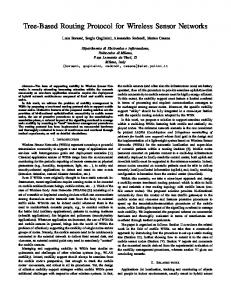
that, the RL algorithms assigns credit to actions based on reinforcement from the environment (Fig 2). Fig. 2. Agent's learning from the environment. In the case ...
1 Wireless Networks Inductive Routing Based on Reinforcement Learning Paradigms Abdelhamid Mellouk
Network &Telecom Dept and LiSSi Laboratory University Paris-Est Creteil (UPEC), IUT Creteil/Vitry, France 1. Introduction Wireless networks, especially Sensor ones (WSN), are a promising technology to monitor and collect specific measures in any environment. Several applications have already been envisioned, in a wide range of areas such as military, commercial, emergency, biology and health care applications. A sensor is a physical component able to accomplish three tasks: identify a physical quantity, treat any such information, and transmit this information to a sink (Kumar et al., 2008; Buford et al., 2009; Olfati-Saber et al., 2007). Needs for QoS to guarantee the quality of real time services must take into account not only the static network parameters but also the dynamic ones. Therefore, QoS measures should be introduced to the network so that quality of real time services can be guaranteed. The most popular formulation of the optimal distributed routing problem in a data network is based on a multicommodity flow optimization whereby a separate objective function is minimized with respect to the types of flow subjected to multicommodity flow constraints. Given the complexity of this problem, due to the diversity of the QoS constraints, we focus our attention in this paper on bio-inspired QoS routing policies based on the Reinforcement Learning paradigm applied to Wireless Sensor Networks. Many research works focus on the optimization of the energy consumption in sensor networks, as it directly affects the network lifetime. Routing protocols were proposed to minimize energy consumption while providing the necessary coverage and connectivity for the nodes to send data to the sink. Other routing protocols have also been proposed in WSN to improve other QoS constraints such as delay. The problem here is that the complexity of routing protocols increases dramatically with the integration of more than one QoS parameter. Indeed, determining a QoS route that satisfies two or more non-correlated constraints (for example, delay and bandwidth) is an NPcomplete problem (Mellouk et al., 2007), because the Multi-Constrained Optimal path problem cannot be solved in polynomial time. Therefore, research focus has shifted to the development of pseudopolynomial time algorithms, heuristics, and approximation algorithms for multi-constrained QoS paths. In this chapter, we present an accurate description of the current state-of-the-art and give an overview of our work in the use of reinforcement learning concepts focused on Wireless Sensor Networks. We focus our attention by developing systems based on this paradigm called AMDR and EDAR. Basically, these inductive approaches selects routes based on flow
2
Advances in Reinforcement Learning
QoS requirements and network resource availability. After developing in section 2 the concept of routing in wireless sensor networks, we present in section 3 the family of inductive approaches. After, we present in two sections our works based on reinforcement learning approaches. Last section concludes and gives some perspectives of this work.
2. Routing problem in Wireless Sensor Networks Goal aspects that are identified as more suitable to optimize in WSNs are QoS metrics. Sensor nodes essentially move small amounts of data (bits) from one place to another. Therefore, equilibrium should be defined in QoS and energy consumption, to obtain meaningful information of data transmitted. Energy efficiency is an evident optimization metric in WSNs. More generally, several routing protocols in WSNs are influenced by several factors: Minimum life of the system: In some cases, no human intervention is possible. Batteries of sensors can not be changed; the lifetime of the network must be maximized. Fault tolerance: Sensor network should be tolerant to nodes failures so as the network routes information through other nodes. Delay: Delay metric must be taken into account for real-time applications to ensure that data arrives on time. Scalability: Routing protocols must be extendable, even with several thousand nodes. Coverage: In WSN, each sensor node obtains a certain view of the environment. This latter is limited both in range and in accuracy (fig. 1); it can only cover a limited physical area of the environment. Hence, area coverage is also an important design parameter in WSNs. Each node receives a local view of its environment, limited by its scope and accuracy. The coverage of a large area is composed by the union of several smaller coverages. Connectivity: Most WSNs have high density of sensors, thus precluding isolation of nodes. However, deployment, mobility and failures vary the topology of the network, so connectivity is not always assured (Tran et al., 2008). Quality of Service: In some applications, data should be delivered within certain period of time from the moment it is sensed; otherwise the data will be useless. Therefore bounded latency for data delivery is another condition for time-constrained applications. However, in many applications, energy saving -which is directly related to the network’s lifetime- is considered relatively more important than the quality of the transmitted data. As the energy gets depleted, the network may be required to reduce the quality of the results in order to reduce energy dissipation in nodes and hence lengthen network lifetime. Hence, energyaware routing protocols are required to capture this requirement.
Fig. 1. Radius of reception of a sensor node.
Wireless Networks Inductive Routing Based on Reinforcement Learning Paradigms
3
To ensure these aspects, one can find two methods to routing information from a sensor network to a sink: Reactive (requested): If one wants to have the network status at a time t, the sink broadcasts a request throughout the network so that sensors send their latest information back to the sink. The information is then forwarded in multi-hop manner to the sink (Shearer, 2008). Proactive (periodical): The network is monitored to detect any changes, sending broadcasts periodically to the sink, following an event in the network such as a sudden change in temperature and movement. Sensors near the event then back the information recorded and route it to the sink (Lu & Sheu, 2007). Otherwise, depending on the network structure, routing can be divided into flat-based routing, hierarchical-based routing, and location-based routing. All these protocols can be classified into multi-path based, query-based, negotiation-based, QoS-based, or coherentbased routing techniques depending on the protocol operation. Below, we present some QoS routing protocols: QoS_AODV (Perkins et al., 2000): The link cost used in this protocol is formulated as a function which takes into account node’s energy consumed and error rate. Based on an extended version of Dijkstra's algorithm, the protocol establishes a list of paths with minimal cost. Then, the one with the best cost is selected [10],[13]. This protocol uses hierarchical routing; it divides the network into clusters. Each cluster consists of sensor nodes and one cluster head. The cluster head retrieves data from the cluster and sends it to the sink. QoS routing is done locally in each cluster. Sequential Assignment Routing (SAR) (Ok et al., 2009): SAR manages multi-paths in a routing table which attempts to achieve energy efficiency and fault tolerance. SAR considers trees of QoS criteria during the exploration of routing paths, the energy resource on each path and the priority level of each packet. By using these trees, multiple paths of the sensors are well trained. One of these paths is chosen depending on energy resources and QoS of path. SAR maintains multiple paths from nodes to sink [9]. High overhead is generated to maintain tables and states at each sensor. Energy Aware Routing (EAR) (Shah & Rabaey, 2002): EAR is a reactive routing protocol designed to increase the lifetime of sensor networks. Like EDAR, the sink searches and maintains multiple paths to the destinations, and assigns a probability to each of these paths. The probability of a node is set to be inversely proportional to its cost in terms of energy. When a node routes a packet, it chooses one of the available paths according to their probabilities. Therefore, packets can be routed along different paths and the nodes’ energy will be fairly consumed among the different nodes. This technique keeps a node from being over-utilized, which would quickly lead to energy starvation. SPEED (Ok et al., 2009): This protocol provides a time limit beyond which the information is not taken into account. It introduces the concept of "real time" in wireless sensor networks. Its purpose is to ensure a certain speed for each packet in the network. Each application considers the end-to-end delay of packets by dividing the distance from the sink by the speed of packet before deciding to accept or reject a packet. Here, each node maintains information of its neighbors and uses geographic information to find the paths. SPEED can avoid congestion under heavy network load.
3. State dependent routing approaches Modern communication networks is becoming a large complex distributed system composed by higher interoperating complex sub-systems based on several dynamic
4
Advances in Reinforcement Learning
parameters. The drivers of this growth have included changes in technology and changes in regulation. In this context, the famous methodology approach that allows us to formulate this problem is dynamic programming which, however, is very complex to be solved exactly. The most popular formulation of the optimal distributed routing problem in a data network is based on a multicommodity flow optimization whereby a separable objective function is minimized with respect to the types of flow subject to multicommodity flow constraints (Gallager, 1977; Ozdaglar & Bertsekas, 2003). In order to design adaptive algorithms for dynamic networks routing problems, many of works are largely oriented and based on the Reinforcement Learning (RL) notion (Sutton & Barto, 1997). The salient feature of RL algorithms is the nature of their routing table entries which are probabilistic. In such algorithms, to improve the routing decision quality, a router tries out different links to see if they produce good routes. This mode of operation is called exploration. Information learnt during this exploration phase is used to take future decisions. This mode of operation is called exploitation. Both exploration and exploitation phases are necessary for effective routing and the choice of the outgoing interface is the action taken by the router. In RL algorithms, those learning and evaluation modes are assumed to happen continually. Note that, the RL algorithms assigns credit to actions based on reinforcement from the environment (Fig 2).
Fig. 2. Agent’s learning from the environment. In the case where such credit assignment is conducted systematically over large number of routing decisions, so that all actions have been sufficiently explored, RL algorithms converge to solve stochastic shortest path routing problems. Finally, algorithms for RL are distributed algorithms that take into account the dynamics of the network where initially no model of the network dynamics is assumed to be given. Then, the RL algorithm has to sample, estimate and build the model of pertinent aspects of the environment. Many of works has done to investigate the use of inductive approaches based on artificial neuronal intelligence together with biologically inspired techniques such as reinforcement learning and genetic algorithms, to control network behavior in real-time so as to provide users with the QoS that they request, and to improve network provide robustness and resilience. For example, we can note the following approaches based on RL paradigm: Q-Routing approach- In this technique (Boyan & Littman, 1994), each node makes its routing decision based on the local routing information, represented as a table of Q values
Wireless Networks Inductive Routing Based on Reinforcement Learning Paradigms
5
which estimate the quality of the alternative routes. These values are updated each time the node sends a packet to one of its neighbors. However, when a Q value is not updated for a long time, it does not necessarily reflect the current state of the network and hence a routing decision based on such an unreliable Q value will not be accurate. The update rule in QRouting does not take into account the reliability of the estimated or updated Q value because it depends on the traffic pattern, and load levels. In fact, most of the Q values in the network are unreliable. For this purpose, other algorithms have been proposed like Confidence based Q-Routing (CQ-Routing) or Confidence based Dual Reinforcement QRouting (DRQ-Routing). Cognitive Packet Networks (CPN)- CPNs (Gelenbe et al., 2002) are based on random neural networks. These are store-and-forward packet networks in which intelligence is constructed into the packets, rather than at the routers or in the high-level protocols. CPN is then a reliable packet network infrastructure, which incorporates packet loss and delays directly into user QoS criteria and use these criteria to conduct routing. Cognitive packet networks carry three major types of packets: smart packets, dumb packets and acknowledgments (ACK). Smart or cognitive packets route themselves, they learn to avoid link and node failures and congestion and to avoid being lost. They learn from their own observations about the network and/or from the experience of other packets. They rely minimally on routers. The major drawback of algorithms based on cognitive packet networks is the convergence time, which is very important when the network is heavily loaded. Swarm Ant Colony Optimization (AntNet)- Ants routing algorithms (Dorigo & Stüzle, 2004) are inspired by dynamics of how ant colonies learn the shortest route to food source using very little state and computation. Instead of having fixed next-hop value, the routing table will have multiple next-hop choices for a destination, with each candidate associated with a possibility, which indicates the goodness of choosing this hop as the next hop in favor to form the shortest path. Given a specified source node and destination node, the source node will send out some kind of ant packets based on the possibility entries on its own routing table. Those ants will explore the routes in the network. They can memory the hops they have passed. When an ant packet reaches the destination node, the ant packet will return to the source node along the same route. Along the way back to the destination node, the ant packet will change the routing table for every node it passes by. The rules of updating the routing tables are: increase the possibility of the hop it comes from while decrease the possibilities of other candidates. Ants approach is immune to the sub-optimal route problem since it explores, at all times, all paths of the network. Although, the traffic generated by ant algorithms is more important than the traffic of the concurrent approaches. AntHocNet (Di Caro et al., 2005) is an algorithm for routing in mobile ad hoc networks. It is a hybrid algorithm, which combines reactive route setup with proactive route probing, maintenance and improvement. It does not maintain routes to all possible destinations at all times but only sets up paths when they are needed at the start of a data session. This is done in a reactive route setup phase, where ant agents called reactive forward ants are launched by the source in order to find multiple paths to the destination, and backward ants return to the source to set up the paths in the form of pheromone tables indicating their respective quality. After the route setup, data packets are routed stochastically over the different paths following these pheromone tables. While the data session is going on, the paths are monitored, maintained and improved proactively using different agents, called proactive forward ants.
6
Advances in Reinforcement Learning
BeeAdHoc (Wedde et al., 2005) is a new routing algorithm for energy efficient routing in mobile ad hoc networks. This algorithm is inspired by the foraging principles of honey bees. The algorithm utilizes Essentialy two types of agents, scouts and foragers, for doing routing in mobile ad hoc networks. BeeAdHoc is a reactive source routing algorithm and it consumes less energy as compared to existing state-of-theart routing algorithms because it utilizes less control packets to do routing. KOQRA (Mellouk et al., 2008; Mellouk et al., 2009) is an adaptive routing algorithm that improves the Quality of Service in terms of cost link path and end-to-end delay. This algorithm is based on a Dijkstra multipath routing approach combined with the Q-routing reinforcement learning. The learning algorithm is based on founding K best paths in terms of cumulative link cost and the optimization of the average delivery time on these paths. A load balancing policy depending on a dynamical traffic path probability distribution function is also introduced.
4. AMDR protocol: Adaptive Mean Delay Routing protocol Our first proposal, called “AMDR” (Adaptive Mean Delay Routing), is based on an adaptive approach using mean delay estimated proactively by each node. AMDR is built around two modules: Delay Estimation Module (DEM) and Adaptive Routing Module (ARM). In order to optimize delay in mobile ad hoc networks, it’s necessary to be able to evaluate delay in accurate way. We consider in DEM, the IEEE 802.11 protocol, which is considered to be the most popular MAC protocol in MANET. DEM calculates proactively mean delay at each node without any packets exchange. The ARM will then exploit mean delay value. It uses two exploration agents to discover best available routes between a given pair of nodes (s, d). Exploration agents gather mean delay information available at each visited node and calculate the overall delay between source and destination. According to delay value gathered, a reinforcement signal is calculated and probabilistic routing tables are updated at each intermediate node using an appropriate reinforcement signal. ARM ensures an adaptive routing based on estimated mean delay. It combines, on demand approach used at starting phase of exploration process (generation of the first exploration packet for the destination) with proactive approach in order to continue the exploration process even a route is already available for the destination. Proactive exploration keeps AMDR more reactive by having more recent information about network state. 4.1 Delay Estimation Model (DEM) In order to optimize delay in mobile ad hoc networks, it’s necessary to be able to evaluate delay in an accurate way. We propose in this section to estimate one-hop delay in ad hoc networks. It’s well known that node delay depends greatly on MAC layer protocol. We consider in our study, the particular case of IEEE 802.11 protocol. Our Delay Estimation Model (DEM) is based on Little’s theorem (Little, 1961). Each mobile node, in DEM, is considered as a buffer. Packets arrive to the buffer in Poisson distribution with parameter λ. Each mobile node has a single server performing channel access. Thus, a mobile node is seen as a discrete time M/G/1 queue (Saaty, 1961). According to Little’s theorem, node delay corresponds to mean response delay defined as fellow:
Wireless Networks Inductive Routing Based on Reinforcement Learning Paradigms
W= • •
λ M2 +b 2(1 − σ )
7 (1)
λ: arriving rate of data packets to the buffer
b: represents mean service time needed to transmit a data packet with success including retransmission delays σ: represents server’s rate occupation, it’s equal to λb • • M2: is the second moment of service time distribution. The generator function of delay service defined in (Meraihi, 2005) is noted B(z, L,p,k), (L : packet size, p : collision rate and k: backoff stage). This generator function can be defined in recursive manner as fellow: B ( z , L , p , k ) = Tx ( z , k , L ) ( 1 − p + p * B ( z , L , p , 2 k ) )
(2)
Tx(z,k,L) is a transmission delay of a data packet (packet size: L). B(z, L, p, 2k) function is invoked in case of collision with a probability p. In order to differentiate link’s delays, we know that collision rate p is different from one neighbor to another. Thus, collision rate becomes a very important parameter for mean delay estimation. 4.2 Adaptive Routing Module (ARM) AMDR uses two kinds of agents: Forward Exploration Packets (FEP) and Backward Exploration Packets (BEP). Routing in AMDR is determined by simple interactions between forward and backward exploration agents. Forward agents report network delay conditions to the backward ones. ARM consists of three parts: 4.2.1 Neighborhood discovery Each mobile node has to detect the neighbor nodes with which it has a direct link. For this, each node broadcasts periodically Hello messages, containing the list of known neighbors and their link status. The link status can be either symmetric (if communication is possible in both directions) or asymmetric (if communication is possible only in one direction). Thus, Hello messages enable each node to detect its one-hop neighbors, as well as its two-hop neighbors (the neighbors of its neighbors). The Hello messages are received by all one-hop neighbors, but are forwarded only by a set of nodes calculated by an appropriate optimization-flooding algorithm. 4.2.2 Exploration process So, FEP agents do not perform any updates of routing tables. They only gather the useful information that will be used to generate backward agents. BEP agents update routing tables of intermediate nodes using new available mean delay information. New probabilities are calculated according to a reinforcement-learning signal. Forward agent explores the paths of the network, for the first time in reactive manner, but it continues exploration process proactively. FEP agents create a probability distribution entry at each node for all its delay-MPR neighbours. Backward agents are sent to propagate the information collected by forward agents through the network, and to adjust the routing table entries. Probabilistic routing tables are used in AMDR. Each routing table entry has the following form (Fig. 3):
8
Advances in Reinforcement Learning
Dest
(Next1, p1)
(Next2, p2)
…..
(Nextn, pn)
Fig. 3. AMDR’s routing table entry. When a new traffic arrives at source node s, periodically this node generates a Forward Exploration Packet called FEP. The FEP packet is then sent to the destination in broadcast manner. Each forward agent packet contains the following informations: Source node address, Destination node address, Next hop address, Stack of visiting nodes, Total_Delay. If the entry of the current destination does not exist when the forward agent is created, then a routing table entry is immediately created. The stack field contains the addresses of nodes traversed by forward agent packet and their mean delay. The FEP sending algorithm is the following: Algorithm (Send FEP) At Each T_interval_seconds Do Begin Generate a FEP If any entry for this destination Then Create an entry with uniform probabilities. End If Broadcast the FEP End End (Send FEP) When a FEP arrives to a node i, it checks if the address of the node i is not equal to the destination address contained in the FEP agent then the FEP packet will be forwarded. FEP packets are forwarded according to the following algorithm: Algorithm (Receive FEP) If any entry for this destination Then Create an entry with uniform probabilities Else If my_adress ≠ dest_adress Then If FEP not already received Then Store address of the current node, Recover the available mean delay, Broadcast FEP, Else Send BEP End If End If End (forward FEP) Backward Exploration Packet As soon as a forward agent FEP reaches its destination, a backward agent called BEP is generated and the forward agent FEP is destroyed. BEP inherits then the stack and the total delay information contained in the forward agent. We define five options for our algorithm in order to reply to a FEP agent. The algorithm of sending a BEP packet depends on the chosen option. The five options considered in our protocol are:
Wireless Networks Inductive Routing Based on Reinforcement Learning Paradigms
9
Reply to All: for each reception of a FEP packet, the destination node generates a BEP packet which retraces the inverse path of the FEP packet. In this case, the delay information is not used and the overhead generated is very important. Reply to First: Only one BEP agent is generated for a FEP packet. It’s the case of instantaneous delay because the first FEP arriving to destination has the best instantaneous delay. The mean delay module is not exploited. It’s the same approach used in the AntNet. The overhead is reduced but any guarantee to have the best delay paths. Reply to N: We define an integer N, stored at each node, while N is positive the destination reply by generating a BEP. It is an intermediate solution between Reply to all and Reply to First (N=1). The variable N is decremented when a BEP is sent. The overhead is more important than The Reply to First option. Reply to the Best: We save at each node the information of the best delay called Node.Total_delay. When the first FEP arrives to the destination, Node.Total_delay takes the value of total delay of the FEP packet. When another FEP arrives, we compare its FEP.Total_delay with the Node.Total_delay, and we reply only if the FEP has a delay better or equal to the Node.Total_delay. In such manner, we are sure that we adjust routing tables according to the best delay. We have a guarantee of the best delay with reduced overhead. If the FEP_Total_delay is equal or less than a fixed value D, the BEP is generated and sent to the source of the FEP. The algorithm of sending a BEP is the following: Algorithm (send BEP) Select Case Option Case: Reply to All Genarate BEP BEP.Total_Delay=0, BEP.dest = FEP.src, Send BEP Case: Reply to first If (First (FEP) ) Then Genarate BEP BEP.Total_Delay=0, BEP.dest = FEP.src, Send BEP endIf Case: Reply to N If (N>0) Then Genarate BEP BEP.Total_Delay=0, BEP.dest = FEP.src, Send BEP, N=N-1 endIf Case: Reply to Best If (FEP.Total_Delay