Rules and Local Function Networks Robert Andrews & Shlomo Geva Neurocomputing Research Centre Queensland University of Technology GPO Box 2434 Brisbane, Q. 4001 Australia
[email protected] [email protected]
Abstract: This paper presents an overview of rule extraction and rule refinement techniques that have been developed specifically for use with local function networks. Local function networks are artificial neural networks that make use of some form of local response units in their hidden layer. Networks that fall into this category include Radial Basis Function, (RBF), networks, the Rapid BackProp, (RBP), network, and the Rectangular Basis Function, (RecBF), network. Techniques to be discussed include those described by Tresp, Hollatz & Ahmad for rule extraction/refinement from RBF networks, Berthold & Huber for rule extraction from RecBF networks, and the RULEX algorithm described by Andrews & Geva for rule extraction/refinement from RBP networks. The paper also addresses advantages and disadvantages of local solutions.
Introduction
In nature there are several examples of neurons with 'local response' characteristics. Here local response is taken to mean that the neuron responds to only a selective range of possible values of the input variable. For example the cochlear stereocilia cells are locally tuned to frequency, cells in the somatosensory cortex respond selectively to stimulation from localised regions of the body surface, and the orientation-selective cells in the visual cortex respond selectively to stimulation which is local in both retinal position and angle of object orientation. Further, populations of locally responsive cells are typically arranged in cortical maps in which the values of the variables to which the cells respond vary with position in the map. [10] In the field of Artificial Neural Networks, (ANNs), there are several types of networks that utilise units with local response characteristics to solve the interpolation, (function approximation), problem.1 Classification, a common application of ANNs, is also an example of interpolation. Poggio & Girosi, [11], discuss the validity of using Radial Basis Functions, (RBF), to solve the interpolation problem. They show that an expansion of the 1
where the interpolation problem is "given values of an unknown function, f, corresponding to certain values of x , what is the behaviour of this function?". We would really like to answer the question "what is this function?", but this is not possible to determine with only a limited amount of data.
form ...(1)
where h( t) is completely monotonic can be used for interpolation. A list of functions that can be used for interpolation are (gaussian)
(α > 0)
(0 < β < 1)
(multiquadratic)
(linear)
Of these, the gaussian function has been most commonly used in RBF networks. Experimental results from RBF networks using some of the above functions can be found in [10] [14] [5] [12] . Lapedes & Faber, [9] give a method for constructing locally responsive units using pairs of axis parallel sigmoids. The local response region is created by subtracting the value of one sigmoid from the other. They did not however offer a training scheme for networks constructed of such units. Geva & Sitte, [7],[8] described a parameterisation and training scheme for networks composed of such sigmoid based hidden units and Geva and Andrews, [1] [2], showed how these networks can be structured to facilitate rule extraction.
Figure 1
Figure 2
Figure 3
Figure 4
In the ith dimension, the sigmoids are paramaterised according to centre, ci , breadth, bi , and edge steepness, ki . The pairs of sigmoids are given by the equations ...(2)
...(3)
where x is the input vector, c is the reference vector, b represents the effective widths of each ridge, and k represents the edge steepness of each ridge. The combination U i+ - U i- forms a ridge parallel to the axis in the ith dimension. (See Figures 1 & 2 above.) The intersection of N such ridges forms a local peak at the point of intersection but with secondary ridges extending away to infinity on each side of the peak. (See Figure 3 above). These ridges can be 'cut off' by the application of a suitable sigmoid to leave a locally responsive region. (See Figure 4 above.) The activation for this sigmoid is given by ...(4)
where B is set to the dimensionality of the input domain and K is set in the range 4-8. The network output is ...(5)
An incremental, constructive training algorithm is used with training, (for rule extraction), involving adjusting, by gradient descent, the centre, ci, breadth, bi, and edge steepness, ki, parameters of the sigmoids that define the local response units. The output weight, w , is held constant. In classification problems where the desired output is either 0 or 1 this measure forces the bumps to avoid overlapping.
The advantage of this is that each bump can then be decompiled into a rule, in isolation of all bumps, in a computationally efficient manner. Typically decompositional methods of rule extraction employ an 'exhaustive search and test' strategy to formulate a rule that describes the behaviour of each individual hidden and output unit. These methods are computationally intensive, are generally exponential in the number of inputs, and usually employ some heuristics to limit the search space. [6] [13] Berthold & Huber, [7] [8], structure their Rectangular Basis Function, (RecBF), networks in such a way that there is a one to one correspondence between hidden units and rules. RecBF networks consist of an input layer, a hidden layer of RecBF units, and an output layer with each unit in the output layer representing a class. The hidden units of RecBF networks are constructed as hyper-rectangles with their training algorithm derived from that used to train RBF networks. The hyper-rectangles are parameterised by a reference vector, r , which gives the centre of the rectangle, and two sets of radii, λ*+,-, which defines the corerectangle, and Λ*+,-, which describes the support-rectangle. (See Figure 5 below.)
Figure 5
The core-rectangle includes data points that definitely belong to the class and the boundary of the support-rectangle excludes data points that definitely do not belong to the class. ie, the support-rectangle is just an area where there are no data points. R( ), the activation function for a RecBF unit is:
...(6)
where x represents the input vector, r represents the reference vector of the unit, and σ is a vector representing individual radii in each dimension and A( ) is the Signum activation function: ...(7)
Training the RecBF network is by the Dynamic Decay Algorithm, (DDA), [7]. This algorithm is based on 3 steps: • covered : a new training point lies inside the support-rectangle of an existing RecBF. Extend the core-rectangle of the RecBF to cover the new point • commit: a new pattern is not covered by a RecBF of the correct class. Add a new RecBF with centre the same as the training instance and widths as large as possible to avoid overlapping any existing RecBF. • shrink : a new pattern is incorrectly classified by an existing RecBF. The RecBF's widths are shrunk so that the conflict is resolved. The process of extracting rules from any trained artificial neural network, (ANN), starts with the recognition that knowledge is encoded in the network in the a) the network architecture, b) the activation function associated with each hidden and output unit, and c) a set of (real-valued) numerical parameters called weights. Rule extraction can be defined as the process of interpreting the collective effects a), b) and c) above in some manner that is meaningful to the user of the ANN. Generally the user is a human user and the meaningful interpretation is in the form of a set of if-then... rules. (There is also no reason why the user of the output of an ANN could not be a rule based system itself such as an expert system.) A related task to rule extraction is rule refinement. Rule refinement is a three step process: rule initialisation, network training, rule extraction. Rule Initialisation involves utilising prior knowledge of the problem domain, (generally in the form of rules formulated by an expert in the problem domain), to bias the learning of the network rather than the network starting its learning from tabula rasa. The network can be biased by prestructuring any or all of the network architecture, activation functions, or weights. The refinement aspect comes from the fact that the knowledge used in rule initialisation may be
partially correct, incomplete, or even totally inaccurate. The network training phase is designed to remove the inaccuracies and to fill in the gaps in the knowledge used to initialise the network. This is achieved by training the initialised network with example patterns drawn from the problem domain. Finally, in the rule extraction phase, a set of rules which is consistent with training data is extracted from the trained network. These are the refined rules. Rule refinement allows for a knowledge base which is basically sound to be modified over time in the light of new example patterns without having to begin training from a zero knowledge position every time some new data from the problem domain is collected. The remainder of this paper is arranged as follows. In section 1 we outline the method described by Tresp, Hollatz, and Ahmad for extracting and refining rules from RBF networks. In section 2 we describe our own RULEX algorithm which may be used for both rule extraction and rule refinement. In section 3 we describe the method used by Berthold & Huber for extracting rules from RecBF networks. Section 4 deals with the strengths and weaknesses of local function networks with respect to rule extraction and refinement. 1 Rule Refinement and RB F Networks
Tresp, Hollatz & Ahmad describe a technique for refining an existing rule set. An Artificial Neural Network y=NN(x), which makes a prediction about the state of y given the state of its input x can be instantiated as a set of basis functions, bi(x), where each basis function describes the premise of the rule that results in prediction y. The degree of certainty of the rule premise is given by the value of bi(x) which varies continuously between 0 and 1. The rule conclusion is given by w i(x) and the network architecture is given as: ...(8)
If the w i's are constants and the basis functions chosen are multivariate gaussians, (ie, individual variances in each dimension), equation (8) reduces the network described by Moody and Darken. [10] They show how the basis functions can be parameterised by encoding simple logical if-then expressions as multivariate Gaussians. For instance the rule IF [(x1
≈ a) AND (x ≈ b)] 4
OR (x2
≈ c)
THEN y = d x x2
is encoded as Training can proceed in any of four modes including:
(1)
(2) (3) (4)
Forget, where training data is used to adapt NN init by gradient descent (ie the sooner training stops, the more initial knowledge is
preserved); Freeze, where the initial configuration is frozen (ie if a discrepancy between prediction and data occurs, a new basis function is added); Correct where a parameter is penalised if it deviates from its initial value; and Internal Teacher where the penalty is formulated in terms of the mapping rather than in terms of the parameters.
Classification is performed by applying Bayesian probability and making the assumption that P(x |classk ).P(classk ) ≈ ∑i bik (x ) to obtain
...(9)
Rule extraction is performed by directly decompiling the gaussian (centre : µij , width : δij) pairs to form the rule premise and attaching a certainty factor, w i to the rule. After training is complete, a `pruning' strategy (rule refinement), is employed to arrive at a solution which has the minimum number of basis functions (rules), and the minimum number of conjuncts for each rule. The strategy is shown below. While Error < Threshold Either Prune/Remove Basis Function which has least importance to
the network, (remove the least significant rule) Or Prune Conjuncts by finding the Gaussian with the largest radius and setting this radius to infinity, (effectively removing the associated input dimension from the basis function) Retrain the network till no further improvement in error End While
2 Rule Refinement and RULEX
The parameters that define the local response units of the RBP network can be decompiled into rules of the form: IF THEN
∀ 1 ≤ i ≤ n : xi ∈ [xi lower , xi upper ] Pattern Belongs to the Target Class
...(10)
where xi lower represents the lower limit of activation of the ith ridge and xi upper represents the upper limit of activation of the ith ridge. These values can be calculated from the ridge parameters as: ...(11)
...(12)
RULEX is suitable for both continuous data and discrete data. RULEX also has facilities for reducing the size of the extracted rule set to a minimum number of propositional rules. This is achieved by removing redundant antecedent conditions, use of negations in antecedents, and by removing redundant rules. RULEX and the RBP network can also be used for rule refinement. In turning a propositional if-then rule into the parameters that define a local response unit it is necessary to determine from the rule the active range of each ridge in the unit to be configured. This means setting appropriately the upper and lower bounds of the active range of each ridge, xi lower and xi upper , and then calculating the centre, breath, and steepness parameters, (ci , bi , ki), according to the equations given below. Setting xi lower and xi upper , appropriately involves choosing values such that they 'cut off' the range of antecedent clause values. For discriminating ridges, ie, those ridges that represent input pattern attributes that are used by the unit in classifying input patterns, these required values will be those that are mentioned in the antecedent of the rule to be encoded. For non-discriminating ridges the active range can be set to include all possible input values in the corresponding input dimension. (Non-discriminating ridges will be those that correspond to input pattern attributes that do not appear as antecedent clauses of the rule to be encoded.)
The ridge centre ci , can be calculated as: ...(13)
Now bi is calculated from the centre, ci , xi lower , and the initial ridge steepness, K 0 and is given as: ...(14)
The steepness parameter ki can be calculated as : ...(15)
3 Extracting Rules From RecB F Networks
The main difference between RBF basis functions and RecBF basis functions is that the RecBF hyper-rectangles have finite radii in each input dimension. This allows straightforward interpretation of the RecBF parameters as rules of the form: IF THEN
∀ 1 ≤ i ≤ n : x i ∈ [ r i - λi - , r i - λi + ] Class c
⊂(r
i
- Λi - , r i - Λi + ) ...(16)
Here [ ri - λi- , ri - λi+ ] represents the core-rectangle region of the RecBF unit and ( ri - Λi- , ri - Λi+ ) represents the support-rectangle region of the RecBF unit. Rules of this form have a condition clause for each of the n dimensions of the problem domain. This reduces the comprehensibility of the extracted rule set by including rules which contain antecedents for don't care dimensions, ie, dimensions which the network does use to discriminate between input patterns. Don't care dimensions are those where ri - λi- ≤ xi min and ri - λi+ ≥ xi max where xi min is the smallest possible allowable value of the ith input dimension and xi max is the largest possible allowable value of the ith input dimension. Using the above scheme condition clauses for don't care dimensions are removed from the rules extracted from RecBF networks. One problem associated with RecBF networks is that the DDA training algorithm trains to zero error on the training set. This can result, in the case of noisy data sets or problem domains not suited to description by hyper-rectangles, in a network solution that has a low error rate but which is overtrained on the
data set. This sort of solution will compromise the comprehensibility of the extracted rule set by producing rules that describe exceptions, ie, the noisy data points. To combat this Berthold and Huber use a pruning strategy to reduce the rule set. Rules are pruned until an acceptable compromise is reached between classification accuracy and rule set size. 4 Strengths and Weaknesses of Local Function Networks
From a rule extraction/refinement point of view there are two major strengths of local function networks. Firstly, it is conceptually easy to see how a local response unit can be converted to a symbolic rule. In all cases this conversion is achieved by describing the area of response of the individual units in terms of a reference vector that represents the centre of the unit and a set of radii that determine the effective range of the unit in each input dimension, (and hence the boundaries of the unit). The rule associated with the unit is formed by the conjunct of these effective ranges in each dimension. Rules extracted from each local response unit are thus propositional and of the form: IF (x1 ∈ [ x1 min , x1 max ]) ∧ (x2 ∈ [ x2 min , x2 max ]) ... ∧ (xn ∈ [ xn min , xn max ]) THEN pattern belongs to class c where [ xi min , xi max ] represents the effective range in the ith input dimension. Secondly, because each local response unit can be described by the conjunct of some range of values in each input dimension it makes it easy to add units to the network during training such that the added unit has a meaning that is directly related to the problem domain. In networks that employ incremental learning schemes, (such as RecBF and RBP networks), a new unit is added when there is no significant improvement in the global error. The unit is chosen such that its reference vector, ie, the centre of the unit, is one of the as yet unclassified points in the training set. Thus the premise of the rule that describes the new unit is the conjunction of the attribute values of the data point with the rule consequent being the class to which the point belongs. This also makes local function networks suitable for rule refinement. As long as the knowledge to be used for network initialisation can be stated in the form shown above, the starting configuration of the network is given by forming a local response unit for each rule in the knowledge base. A further advantage of local response units over symbolic methods in particular is that when continuous values are quantised (eg [1,10]→{1,2,...10}) the local response units will tend to generalise over a sub range if there is no conflicting data in the middle. For example, a ridge on a value of say 3, can extend to
cover the range 3..7 even if the data does not contain evidence for some value in between. Symbolic methods such as decision trees leave 'holes' and need pruning to recover generalisation. The RecBF makes this property explicit with its core-rectangles and support-rectangles. The property is also apparent in the RBP networks where the local function ridges will grow through an area of no conflicting data Only establishing boundaries when patterns that don't belong to the target class are encountered. There are also disadvantages associated with local function networks. By definition, the rules extracted from such networks are themselves local in nature which makes the explanation of problems such as the Twin Spiral, or Chess Board, which are inherently non-local problems, difficult. The rule set extracted from the network may be accurate in terms of data points classified, however the local nature of the extracted rules will hide from the reader the underlying problem description. As a simple example consider the problem shown in Figure 6 below. The x 's represent patterns that belong to the target class while the o 's represent patterns that do not belong to the target class.
Figure 6
Figure 7
The boxes shown in Figure 7 represent local functions. Clearly the solution is accurate but the extracted rules that describe the local functions will mask the fact that the underlying relationship is simple, viz, a noisy d2 = md1 + c (where m and c are constants). Another problem is that caused by overlapping local response units. One of the nice features of rule extraction from local response units is the ease with which the unit can be directly decompiled into a rule. This obviates the necessity for exhaustive search and test strategies as employed by other rule extraction methods. Thus the computational effort required to extract rules from local response units is significantly less than that required to extract rules using other methods. However, the above is true only so long as the local response units do not
overlap, ie, if a pattern is classified into the target class then exactly one local
response unit shows significant activation. If local response units are allowed to overlap more than one unit will show significant activation when presented with an input pattern. The pattern will be classified by the network , but when the individual units are decompiled into rules, these rules may not account for the pattern/s that fell in the region of overlap. (See Figure 8 below.)
Figure 8
There are essentially two strategies that can be employed when solving the overlap problem. The first is to allow the network to produce overlapping local response units and then deal with this in the rule extraction phase. This is the strategy employed by Tresp, Hollatz and Ahmad, [14]. This will result in rules with a certainty factor attached, ie, fuzzy rules. The other approach to the problem is that employed by both the RecBF networks and the RBP networks, ie, do not allow overlap to occur. This method certainly makes the rule extraction process easy and ensures that every pattern classified by the network is accounted for in the extracted rule set, but the cost may be that the network forms a less than optimum solution to the problem. The related issues of generalisation and regularisation should also be addressed. The assumption is often made, (in classification problems at least), that if the pattern to be classified is not in class 1 then it is, by default, in class 0. There is rarely enough evidence in the training data to support this assumption. In most problems, (and in high dimensional problems in particular), the patterns used in training will not cover the entire input space. Consider the case illustrated in Figure 9 below. The x's represent patterns that belong to class 1, the o 's represent patterns that belong to class 0, and the ? 's represent areas of input space not represented in the pattern set. The network is being trained on class 1.
Figure 9
In solutions which allow the local functions to grow in the absence of conflicting evidence, at least the following solutions are possible.
Figure 10
Figure 11
Both the solutions shown in Figures 10 & 11 make generalisations about regions of input space for which there is no supporting evidence in the pattern set. These solutions may prove acceptable however because they seem to describe some regularity in the data. A solution such as that shown in Figure 12 below, which fits the data equally as well and also explains only regions about which evidence has been provided, may not prove as acceptable because it is not as 'simple' and does not show any regularity in the data.
Figure 12
Conclusion
In this paper we have discussed three different types of local function networks and the techniques used for rule extraction/refinement from each of these networks. We showed that each of these networks is underpinned by a sound theoretical base and that the techniques for rule extraction/refinement from these networks are theoretically sound. We also discussed the pro s and cons of employing local response networks for solving problems requiring interpolation and inductive learning with a view to being able to explain the solution afterwards. Local response networks have been demonstrated to be an effective and efficient tool for problem solving. There are also a number of characteristics inherent in local response units that make them particularly suitable for rule extraction/refinement. The most significant of these is the fact that there is a problem domain relevant meaning that can be attached to each unit thus facilitating not only rule extraction but rule initialisation. A question mark does however hang over the use of rule sets that consist of purely local rules that attempt to explain the network solution to a problem that is non-local in nature. An open research question is finding an efficient method of converting such a set of propositional local rules into a rule set expressed in say first, or higher, order logic where the non-localness is made explicit.
References
[1] [2] [3]
[4] [5] [6]
[7]
[8]
Moody J. & Darken C.J., Fast Learning in Networks of Locally-Tuned Processing Units, Neural Computation 1,MIT, 1989, pp281-94 Poggio T. & Girosi F., A Theory of Networks for Approximation Learning , AI Memo 1140, Massachusetts Institute of Technology, 1989. Lapedes A. & Faber R., How Neural Nets Work, Neural Information Processing Systems (Denver, 1987), Anderson D.Z.(ed), American Institute of Physics, New York, pp442-456. Geva S, & Sitte J., A Constructive Method of Multivariate Function Approximation by MultiLayer Perceptrons, IEEE Transactions on Neural Networks, 1992. Geva S. & Sitte J., Constrained Gradient Descent, Proceedings of the 5th Australian Conference on Neural Computing, Brisbane Australia, 1994. Andrews R. & Geva S.,Extracting Rules From a Constrained Error Backpropagation Network, Proceedings of the 5th Australian Conference on Neural Networks, Brisbane, 1994. Andrews R. & Geva S., RULEX & CEBP Networks as the Basis For a Rule Refinement System , in Hybrid Problems Hybrid Solutions, Hallam J.(Ed), IOS Press, 1995, pp1-12. Berthold M. & Huber K., From Radial to Rectangular Basis Functions: A New Approach for Rule Learning from Large Datasets, Technical Report 15-95, University of Karlsruhe.
[9]
[10] [11] [12] [13] [14]
Berthold M. & Huber K., Building Precise Classifiers with Automatic Rule Extraction , Proceedings of the IEEE International Conference on Neural Networks, Perth, Australia, 1995, Vol3 pp1263-1268. Roschein M., Hofmann R. & Tresp V., Incorporating Prior Knowledge in Parsimonious Networks of Locally Tuned Units, Tech Report TR FKI-155-91. Tresp V, Hollatz J. & Ahmad S., Network Structuring and Training Using Rule-Based Knowledge, In Neural Information Processing Systems (1993), pp871-878. Broomhead D. & Lowe, Multivariable Function Interpolation and Adaptive Networks, Complex Systems, 2:321-355, 1988. Towell G. & Shavlik J., Extracting Refined Rules From Knowledge Based Neural Networks, Machine Learning, October 1993, Vol3 No1 pp71-101. Fu L., Rule Generation From Neural Networks, IEEE Transactions on Systems, man and Cybernetics, August 1994, Vol24 No8, pp1114-1124.