specifically, the MTTR of a software service is defined as the average time from a failure of a service to respond to an operation call until it restarts responding to ...
Runtime Prediction of Software Service Availability Davide Lorenzoli, George Spanoudakis Department of Computing, City University London, London, UK Abstract This paper presents a prediction model for software service availability measured by the mean-time-to-repair (MTTR) and mean-time-to-failure (MTTF) of a service. The prediction model is based on the experimental identification of probability distribution functions for variables that affect MTTR/MTTF and has been implemented using a framework that we have developed to support monitoring and prediction of quality-of-service properties, called EVEREST+. An initial experimental evaluation of the model is presented in the paper. Keywords: Run-time QoS Prediction, Software Services
1
Introduction
The monitoring of quality-of-service (QoS) properties of software services at runtime is supported by several approaches (see [2] for a survey). Most of these approaches, however, can only detect violations of QoS properties after they have occurred without being able to predict them. This is a significant limitation as the capability to predict violations of QoS properties at runtime is important for the dynamic and proactive adaptation of both the services and the systems that use them. The prediction of QoS properties violations is a challenging problem. This is because there is often a lack of models (e.g., service behavioural models, deployment infrastructure models) that would enable a white-box approach to prediction based on analytic techniques (e.g. [21]). Hence, QoS property prediction has often to rely on black-box techniques analysing QoS service data collected at runtime. In this paper, we present a runtime prediction model for a key QoS property of software services, namely software service availability. The model is based on the prediction of two measures of service availability: the mean-time-to-failure (MTTF) and mean-time-to-repair (MTTR) of a software service, defined as the average up and down time in the operational life of a service, respectively [19][20]. Our MTTR/MTTF prediction model is based on the experimental identification of probability distribution functions for the variables that affect these two measures. The MTTR/MTTF model has been implemented using an integrated framework that we have developed to support monitoring and prediction of QoS properties of software services expressed in service level agreements (SLAs), called EVEREST+. EVEREST+ enables the monitoring of QoS and behavioural service properties expressed in Event Calculus, and the development and automatic maintenance of runtime models for estimating the probability of potential violation/satisfaction of constraints over such properties (i.e., prediction models).
The development of prediction models in EVEREST+ is based on prediction specifications determining: (a) the key variables underpinning the QoS properties that need to be predicted, (b) the patterns of events that need to be monitored in order to collect runtime data about these variables, and (c) the computations that need to be performed to generate predictions for the properties. Based on these specifications, EVEREST+ can infer automatically the probability distribution functions of the variables that underpin the QoS properties of interest at runtime using monitoring data, and uses these functions to calculate the probability of future violations of the QoS properties. The rest of this paper is structured as follows. In Sect. 2, we describe the prediction model for software service MTTR and MTTF. In Sect. 3, we describe how the MTTR/MTTF models are realised in EVEREST+. In Sect. 4, we present the results of an initial experimental evaluation of the prediction model. Finally, in Sect. 5 we discuss related work and in Sect. 6, we present concluding remarks and directions for future work.
2
Prediction Model
2.1 Overview A QoS property prediction in our approach is the computation of the probability that the QoS property will violate a constraint at some future time point te, given a request for it received at a time point tc. Figure 1 illustrates this general formulation of the prediction problem. In particular, tc in the figure is the time point at which a prediction for a property QoS is requested; te is the time point in the future that the prediction is required for; p is the prediction window (i.e., p=te−tc); N is the number of QoS values observed between ts and tc; Y is the number of future QoS property values that are expected between tc and ts; QoSc is the value of the observed QoS property at the time point tc; and QoSy is the value of the predicted QoS property at the time point te. "#$%&'()*!+,-&!
/#$%&'()*!+,-&! !"#$!
!&!
!"#%!
!0!
!'!
!!
.!
Figure 1. Prediction framework common definitions Given this generic formulation, the computation of the probability of violating a QoS property constraint is based on estimating the probability of occurrence of different values of variables that affect the QoS property in the prediction window, and can make it violate the constraint. The
probabilities of the values of the underpinning variables are determined by finding the probability distribution functions (PDFs) that have the best fit to sets of historic values of these variables. 2.2 Prediction Model for Software Services MTTR The overall approach outlined above has been used to develop the prediction model for the mean-time-to-repair (MTTR) and mean-time-to-failure (MTTF) of a service. More specifically, the MTTR of a software service is defined as the average time from a failure of a service to respond to an operation call until it restarts responding to operation calls normally. MTTR needs to be bounded to ensure the timely reactivation of a service after periods of unavailability. In an SLA, this would be typically specified as a boundary constraint of the form: MTTR ≤ K where K is a constant time measure. The estimation of the probability of violating the boundary constraint MTTR ≤ K at a future time point te is based on identifying the probability distribution functions of two variables: (1) the MTTR of the service of concern, and (2) the time between non-served calls of service operations (i.e., service failures) that occur in a period during which a service has been available (referred to as time-to-failure or “TTF” henceforth). MTTR and TTF values correspond to the periods in the operational life of a service shown in Figure 2. More specifically, MTTR is computed as the average of TTR values, i.e., the time difference between the timestamp of the first served call of a service following a period of unavailability and the timestamp of the initial non served call (NS Call) of the service that initiated this period. TTF is the difference between the timestamps of two NS calls of the service that initiate two distinct and successive periods of unavailability.
*123&'! !+$0.//%,!
""#$%)!
""#$%&!
""#$! !"#$%&'(&)$ *!+, -.//!
+&'(&)! 0.//!
!+$-.//!
*123&'! %&'(&)$0.//%,!
*123&'$! !+$0.//%,!
+&'(&)! 0.//!
!!
'$%&!
' $! ""($!
!+ 0.//!
*123&'! +&'(&)$0.//%,!
""($%&!
""($%)!
Figure 2. TTR and TTF values Assuming that N is the number of MTTR values recorded until the time tc at which the prediction is requested, te is the future time point for which the prediction is requested, and y is the − yet unknown − number of TTF values that will be recorded during the prediction horizon p (or, equivalently, the number of cases where the service fails again following a period over which it has been available), to violate the MTTR constraint at te the following condition must be false: MTTR ! = (N×MTTR ! + y×MTTR ! )/(N + y) ≤ K
TTR ! = N × MTTR ! !!!
TTR ! = y × MTTR ! !!!!!
From formula (1), however, it can be deduced that for the MTTR constraint to be violated it must be that: (2)
MTTR ! ≥ (K × N + y − N × MTTR ! )/y
Given (2), however, there are two factors to take into account to predict MTTR: (a) The probability to observe y reactivations of the service in the time period p from tc to te, denoted as Pr(y) in the following, and (b) The probability of having MTTRy > MTTRcrit (i.e., Pr(MTTRy > MTTRcrit)) where MTTRcrit= (K × (N + y) – N × MTTRc)/y. Based on the probabilities (a) and (b), the probability to violate the constraint MTTR ≤ K at the end of the time period p can be estimated approximately by the following formula: !
1−
!
Pr
!!
=
Pr ! × Pr !""#! ≤ !""#!"#$ ,
!""#! > !
Pr ! × Pr (!""#! > !""#!"#$ ) ,
!""#! ≤ !
!!! !
!!!
(3)
!!!
Formula (3) distinguishes two cases: (a) the case where the last recorded MTTR value at the time when the prediction is requested violates the constraint (i.e., the case where MTTRc >K), and (b) the case where the last recorded MTTR value at the time when the prediction is requested does not violate the constraint (i.e., the case when MTTRc ≤ K). In the former case, the probability of violation is computed as the probability of not seeing a value of MTTR in period p (i.e., MTTRy) that is sufficiently small to restore the current violation. In the second case, the probability of the violation is computed as the probability of seeing a large enough MTTRy value (i.e., a value greater than MTTRcrit) that would violate the constraint. However, since the value of y is not known at tc when the prediction is requested, formula (3) considers values of y up to an upper limit M. The value of M is determined by a condition over its probability. More specifically, M is set to the largest value that makes Pr(y=M) arbitrarily small (i.e., Pr(y=M) MTTRy) we need to know the cumulative distribution functions (CDF) for the variables y and MTTR, referred to as CDFy and CDFMTTR, respectively. Given CDFMTTR, Pr(MTTRcrit >MTTRy) and Pr(MTTRcrit ≤ MTTRy) can be computed by formulas (4) and (5) below:
(1)
According to (1), the MTTR value at te (i.e., MTTRe) is computed by replacing each of the N TTR−values that have been recorded until tc by the average value MTTRc that has been recorded until tc, and each of the y TTR−values from tc to te by their average value MTTRy since:
!!!
!
Pr MTTR !"#$ > MTTR ! = CDF!""# (MTTR !"#$ )
(4)
Pr MTTR !"#$ ≤ MTTR ! = 1 − CDF!""# (MTTR !"#$ )
(5)
To compute Pr(y) we do not use CDFy but the probability distribution function of TTF variable (i.e., the difference between the timestamps of two NS calls of the service that initiate two distinct and successive periods of unavailability, 1
The value of e is set by the requester of the prediction.
as defined earlier). This is because over a time period of p time units TTF is related to y as shown by the formula below:
As (6) indicates, TTF is an invertible monotonic function g of y (i.e., TTF = g(y) = p/y where p is constant). Thus, the cumulative probability distribution of y CDFy = g(CDFTTF) can be computed by the formula: where !
!!
= 1 − !"#!!" !/!
(7)
! = !!" = !/!.
Furthermore, to compute Pr(y), instead of considering a single value v of y, we consider the range ℜ(v) = (v −0.5,v +0.5]. Thus, assuming that x1 = y −0.5 and x2 = y +0.5, Pr(y) is computed by the following formula: !" ! = !"#! !! − !"#! !! = !"#!!" !/!! − !"#!!" !/!!
(8)
In the case of MTTF, the typical SLA constraint that should be monitored and forecasted is MTTF ≥ K (the largest the MTTF the less frequent the failures of the given services) and the probability of violating this constraint can be estimated approximately by the formula: !
1−
!
!′ !
Pr
=
Pr ! × Pr !""!! ≥ !""#!"#$ ,
!""#! < !
!!! !
!!!
(9) Pr ! × Pr !""#! < !""#!"#$ ,
!""#! ≥ !
!!!
The above formula is derived similarly to the case of MTTR but due to space restrictions the details of its derivation are omitted (see [24] for a full account).
3
Prediction Framework !"#$ !"#$ !"#$ %&'()*+"&$ %&'()*+"&$ %&'()*+"&$
(6)
TTF = p/y
!"#! ! = 1 − !"#!!" !!! !
EVEREST+
Runtime Computation Of MTTR/MTTF Models
The prediction models of MTTR and MTTF have been implemented using EVEREST+. EVEREST+ is a generalpurpose framework for monitoring functional and QoS properties of distributed systems at runtime, and developing prediction models for QoS properties. The framework includes two subsystems: (1) a core monitoring subsystem, called EVEREST (EVEnt REaSoning Toolkit [16]), and (2) a prediction subsystem. The monitoring subsystem of EVEREST+ checks functional and QoS properties based on events intercepted from services using internal or external event captors. Whilst monitoring QoS properties, EVEREST stores QoS related information, including computed QoS property values, instances of violations and satisfaction of guaranteed constraints of QoS properties that have been set in SLAs, and the values of any other state variables that might have been taken into account in checking particular QoS properties. These types of information are made available through an API.
!"#$
#45$ 6)"-/3"0$
!"#$ ."0)+"&$
!"#$ 7%'*)8*/3"0$
2&'()*3"0$
Prediction specification - Agreement term - Prediction parameters - Predictor configuration - QoS specification
,"('-$
EVEREST ,"('-$ ./0/1'&$
,"0)+"&)01$ 7%'*)8*/3"0$ 1'0'&/+"&$
2&'()*3"0$ ./0/1'&$
read
write
communication
Figure 3. EVEREST+ Architecture The prediction subsystem of EVEREST+ (see prediction framework in Figure 3) supports the generation of predictions for potential violations of guaranteed constraints for QoS properties upon request. This support is available through generic functionalities including: the automatic fitting of different built-in probability distribution functions (PDFs) to different types of historical QoS data generated by EVEREST; the selection of the PDFs that have the best fit with the data, the update of PDFs following the accumulation of further QoS property monitoring data; and the generation of predictions for QoS property violations based on built-in and/or user defined functions making use of the probabilities returned by the fitted PDFs. EVEREST+ automates the prediction generation process based on prediction specifications expressed in an extension of the SLA specification language SLA* [22] that we have developed for this purpose. 3.1 Prediction Specifications A prediction specification (PS) includes: (a) a set of generic parameters for the forecast, (b) the agreement term to be forecasted, (c) a predictor configuration, and (d) a QoS specification. In the following, we examine these parts of prediction specifications more closely and illustrate them through the example PS shown in Figure 4, which is used to derive the prediction model for MTTR (the grey text within parentheses in the figure shows the differences of the PS for MTTF prediction model). (i) Generic parameters: The generic parameters in a PS determine: the identifier of the service and the operation that the QoS property to be forecasted relates to, the prediction window of forecasts (i.e., the time period in the future that the prediction is required for), and the history size of forecasts (i.e., the size of the historic event set that will be analysed to derive the prediction model). In the example of Figure 4, the PS refers to the operation Ping of service Srv and sets the prediction window to 10 minutes, and the history size to 500 events. (ii) Agreement term: The agreement term in a PS specifies the constraint that should be satisfied for the QoS property of interest by the target service and operation of the PS (aka guaranteed_state). In the example in Figure 4, the guarantee state refers to the QoS property MTTR (MTTF) and the specified constraint regarding is that MTTR (MTTF) must be less than (greater than) 10 seconds.
(iii) Predictor configuration: The predictor configuration in a PS indicates which prediction model to use for computing the probability of the guarantee state of the PS, and the variables whose probability distribution functions will need to be determined from historical monitoring data as they will be needed by the predictor. The former is specified as the value of the attribute predictor.id of the predictor configuration in a PS and the latter are specified by the element prediction variables that includes a list of variables, each of which is specified by a name/value pair. 1 2 3 4 5 6 7 8 9 10 11 12 13 14 15 16 17 18 19 20 21 22 23 24 25 26 27 28 29 30 31 32 33 34 35
prediction_specification { generic_parameters { service.id = Srv operation.id = Ping prediction.window.value = 10 prediction.window.unit = minute history.window.size = 500 history.window.unit = event } agreement_term { guaranteed_state { expression.qos = MTTR (MTTF) expression.operator = less_than (greater_than) expression.value = 10 expression.unit = second } } predictor_configuration { predictor.id = MT_SV_PRED prediction_variables { variable { name = EVEREST+.model.distribution value = MTTR (MTTF) } variable { name = EVEREST+.model.distribution value = TTF } } } qos_specification { specification.name = MTTR (MTTF) specification.value = MTTR-Formulas (MTTF-Formulas) } }
Figure 4. Prediction specification for MTTR/MTTF In Figure 4, the predictor configurator identifies the predictor as “MT_SV_PRED” (i.e., a parametric predictor for formulas (3) and (9) – see Sect. III.C). It also identifies the two variables used as parameters for the two models (i.e., “MTTR” and “TTF” for the MTTR model and “MTTF” and “TTF” for the MTTF model). The names used for the identification of the two prediction parameters of the MTTR model correspond to names of fluent-variables used in the operational monitoring specifications of the relevant QoS properties. Based on this convention, EVEREST+ can identify the monitoring data that need to be considered in determining the probability distributions functions of the relevant variables at runtime, as we explain below. (iv) QoS Specification The QoS specification within a PS provides the operational monitoring specification of the guaranteed state of the QoS property that the prediction is required for. This monitoring specification is expressed in the Event Calculus based monitoring language of EVEREST+, called ECAssertion. A full description of EC-Assertion is beyond the scope of this paper and can be found in [16]. In the following, however, we provide an overview of the language to enable
the reader understand the monitoring specification of MTTR listed below. In EC-Assertion, a guaranteed state over a QoS property is expressed by a monitoring rule and a set of zero or more assumptions. Both monitoring rules and assumptions in have the general form: body⇒head. The semantics of a monitoring rule of this form is that when the body of the rule evaluates to True, its head must also evaluate to True. The semantics of an assumption is that when the body of the assumption evaluates to True, its head can be deduced as a consequence. The body and head of EC-Assertion rules and assumptions are defined in terms of the following Event Calculus predicates: (a)
The predicate Happens(e,t,R(lb,ub)) which denotes that an instantaneous event e occurs at some time t with in the time range R(lb,ub);
(b) The predicate HoldsAt(f,t) which denotes that a state (a.k.a. fluent) f holds at time t; (c)
The predicates Initiates(e,f,t) and Terminates(e,f,t) which denote the initiation and termination of a fluent f by an event e at time t respectively; and
(d) The predicate Initially(f) which denotes that a fluent holds at the start of the operation of a system. The QoS specification of the MTTR of a service _Srv in EC-Assertion is shown in Table 1. The formulas in Table 1 check whether the MTTR is always below a given threshold K. More specifically, the rule R1 checks for the MTTR condition violations when a call of operation _O in service _Srv is served after a period of service unavailability. The first two conditions in the rule (see Happens predicates) check whether the operation call has been served, i.e., whether the service has produced a response to the call within d time units. The third condition of R1 (cf. predicate HoldsAt(Unavailable(_PeriodNumber,_Srv,_STime),t1)) checks whether the served operation call happened at a time when the service has been unavailable, and the fourth condition establishes the MTTR value at the time of the call. The assumption R1.A1 in Table 1 initiates the fluent Unavailable(_PeriodNumber+1,_Srv,t1) to represent a period of service unavailability. This fluent is initiated when a service call occurs (i.e., the call represented by the event _id1) without a response to it within d time units, and at the time of the occurrence of the call the service is not already unavailable (i.e., no fluent of the form Unavailable(_PeriodNumber, _Srv, _STime) already holds). The assumption R1.A2 terminates the fluent that represents a currently active period of service unavailability (i.e., the fluent Unavailable(_PeriodNumber, _Srv, _STime)),when a served service call occurs whilst the service is unavailable. The assumption R1.A3 updates the fluent MTTR(_Srv, _PeriodNumber, _MTTR) that represents the mean length of consecutive periods of service unavailability, i.e., the value of the variable _MTTR of the fluent (note: The formula for the MTTRnew variable in Table 1 is provided separately, to make the specification easier to read. In EVEREST+, this formula should be specified inside the fluent MTTR(…) of the last Initiates predicate of R1.A3).
Run-time prediction
Table 1. QoS Specification of MTTR105
(1) Rule R1: H a p p e n s (e( id1, Snd, Srv,Call( O), Srv),t1 , [t1 ,t1 ]) ∧ H a p p e n s (e( id2, Srv, Snd, Response( O), Srv),t2 , [t1 ,t1 + d]) ∧ ∃ PeriodNumber, STime, MT T R : H o l d s At (Unavailable( PeriodNumber, Srv, STime),t1 ) ∧ H o l d s At (MT T R( Srv, PeriodNumber, MT T R),t1 ) ⇒ MT T R < K
(2) Assumption R1.A1: H a p p e n s (e( id1, Snd, Srv,Call( O), Srv),t1 , [t1 ,t1 ]) ∧ H a p p e n s (e( id2, Srv, Snd, Response( O), Srv),t2 , [t1 ,t1 + d]) ∧ ¬H ¬∃ PeriodNumber, STime, MT T R : H o l d s At (Unavailable( PeriodNumber, Srv, STime),t1 ) ∧ ∃P eriodNumber, MT T R : H o l d s At (MT T R( Srv,P eriodNumber, MT T R),t1) ⇒
I n it i at e s (e( id1, Snd, Srv,Call( O), Srv),Unavailable( PeriodNumber + 1, Srv, STime),t1 ) ∧ T e r m i n at e s (e( id1, Snd, Srv,Call( O), Srv), MT T R( Srv, PeriodNumber, MT T R),t1 ) ∧ I n itprediction i at e s (e( id1, Snd, Srv,Call( O), Srv), MT T R( Srv, PeriodNumber + 1, MT T R),t1 ) Run-time 105
(1) Assumption Rule R1: (3) R1.A2: H aHpappepnes (e( id1, Snd, Srv,Call( O),O), Srv),t ])1 ])∧ ∧ n s (e( id1, Snd, Srv,Call( Srv),t [t1 ,t 1 , [t11, ,t H aHpappepnes (e( id2, Srv, Snd, Response( O),O), Srv),t n s (e( id2, Srv, Snd, Response( Srv),t [t1 ,t+1 d]) + d])∧ ∧ 2 , [t21, ,t ∃ PeriodNumber, STime, MTSTime T R : H: oHl dosl dAst A (Unavailable( PeriodNumber, Srv, STime),t ∃ PeriodNumber, t (Unavailable( PeriodNumber, Srv, STime),t )⇒ 1 ) 1∧ H oSrv),Unavailable( l d s At (MT T R( Srv,PeriodNumber, PeriodNumber,Srv, MTSTime),t T R),t1 ) 1⇒ T e r m i n at e s (e( id1, Snd, Srv,Call( O), ) MT T R < K (4) Assumption R1.A3: (2) Assumption R1.A1: H a p p e n s (e( id1, Snd, Srv,Call( O), Srv),t1 , [t1 ,t1 ]) ∧ H a pSrv, p e n sSnd, (e( id1, Snd, Srv,Call( ,t1 ]) ∧ H a p p e n s (e( id2, Response( O), Srv),tO), ,t1 + d]) 1 , [t1∧ 2 , [t1Srv),t (e( id2, Srv, Snd, Response( O), ∃ PeriodNumber, STime¬H :H Haopl dpseAnts(Unavailable( PeriodNumber, Srv,Srv),t STime),t ∧d]) ∧ 2 , [t1 ,t 1 )1 + ¬∃ PeriodNumber, STime,MT MTTTRR: :HHool lddssAAt t(MT (Unavailable( PeriodNumber,MT Srv, STime),t ∃ PeriodNumber, T R( Srv, PeriodNumber, T R),t 2) ⇒ 1) ∧
∃P eriodNumber, T RSrv), : H oMT l d sA (MT T R( Srv,P eriodNumber, T e r m i n at e s (e( id1, Snd, Srv,Call(MT O), T tR( Srv, PeriodNumber, MT T MT R),tT2 )R),t1) ∧ ⇒ I Innitiitai at et es s(e( 1, TSrv, id1, Snd, Snd, Srv,Call( Srv,Call(O), O), Srv),Unavailable( Srv), MT T R( Srv, PeriodNumber PeriodNumber,+MT RnewSTime),t ),t2 ) (e(id1, 1) ∧ MTSrv), T R( MT PeriodNumber − 1) + (t1 − STime) T e r m i n at e s(e( id1, Snd, Srv,Call( O), T R( Srv, PeriodNumber, MT T R),t1 ) ∧ where MT T Rnew = PeriodNumber I n it i at e s (e( id1, Snd, Srv,Call( O), Srv), MT T R( Srv, PeriodNumber + 1, MT T R),t1 ) (5) Assumption R1.A4: (3) Assumption R1.A2:
A QoS specification Hmust also a O), specification a p p e n s (e( id1, include Snd, Srv,Call( Srv),t , [t ,t ]) ∧ of H a p p e n s (e( id1, Snd, Srv,Call( O), Srv),t1 1 , [t1 1 ,t1 1 ]) ∧ H athat ¬H p p e n sis (e( used id1, Snd,toSrv, Response(the O), Srv),t ]) ∧the 1 , [t1 ,t1of the monitoring pattern record values H a p p e n s (e( id2, Srv, Snd, Response( O), Srv),t 2 , [t1 ,t1 + d]) ∧ ¬∃ PeriodNumber1, STime : H o l d s At (Unavailable( PeriodNumber1, Srv, STime),t1 ) ∧ ∃ PeriodNumber, : H o l d sare At (Unavailable( Srv, STime),t prediction variables,STime which used in PeriodNumber, the prediction model 1 ) ⇒of ∃ PeriodNumber2, T T F lT F : H o l d s At (T T F( PeriodNumber2, Srv, T T F, lFT ),t1 ) ⇒ T e rrelevant m i n at e s (e( id1, O), Srv),Unavailable( Srv, STime),t1 ) of the PSSnd, butSrv,Call( are not forPeriodNumber, the pure monitoring T e r m i n at e s (e( id1, Snd, Srv,Call( O), required Srv), T T F( PeriodNumber2, Srv, T T F, lT F),t1 ) ∧ the property. AnSrv,Call( example ofT Tsuch a variable TTF since I(4) n itAssumption i at e s (e( id1,R1.A3: Snd, O), Srv), F( PeriodNumber2 + 1, is Srv,t 1 − lT F,t 1 ),t1 ) it is required for predictingHthe of future MTTR a p p eprobability n s (e( id1, Snd, Srv,Call( O), Srv),t ∧ 1 , [t1 ,t1 ]) values Fig. 2 EC formula for monitoring MTTR. Please note, MT T R is just a placeholder created for H aMT p pTeRnfor s (e( id2, Snd, Response( + d]) ∧ the 2 , [t1 ,t1Hence, but it ispurposes. not necessary monitoring itself. readability EC requires formula toSrv, be written in-lineMTTR in the O), fluentSrv),t declaration. PeriodNumber, STime : H o l d s At (Unavailable( PeriodNumber, Srv, STime),t1 ) ∧ QoS ∃specification of MTTR includes a specification enabling ∃ PeriodNumber, MT T R : H o l d s At (MT T R( Srv, PeriodNumber, MT T R),t2 ) ⇒ the monitoring of TTF shows the T e r m i n at e s (e( id1, Snd, Srv,Call( values. O), Srv), MTTable T R( Srv, 2PeriodNumber, MT Tassumption R),t2 ) ∧ Srv,Call( for O), Srv), MT T R( Srv, PeriodNumber, MT T Rnew ),t2 ) I n it i ato t e sinitiate (e( id1, Snd, used fluents keeping TTF values (R1.A4). new
new
MT T R( PeriodNumber − 1) + (t1 − STime)
MT T Rnew = Table 2. QoSwhere Specification of MTTR formulas for TTF PeriodNumber (5) Assumption R1.A4: H a p p e n s (e( id1, Snd, Srv,Call( O), Srv),t1 , [t1 ,t1 ]) ∧ H a p p e n s (e( id1, Snd, Srv, Response( O), Srv),t1 , [t1 ,t1 ]) ∧ ¬H ¬∃ PeriodNumber1, STime : H o l d s At (Unavailable( PeriodNumber1, Srv, STime),t1 ) ∧ ∃ PeriodNumber2, T T F lT F : H o l d s At (T T F( PeriodNumber2, Srv, T T F, lFT ),t1 ) ⇒
T e r m i n at e s (e( id1, Snd, Srv,Call( O), Srv), T T F( PeriodNumber2, Srv, T T F, lT F),t1 ) ∧ I n it i at e s (e( id1, Snd, Srv,Call( O), Srv), T T F( PeriodNumber2 + 1, Srv,t1 − lT F,t1 ),t1 ) Fig. 2 EC formula for monitoring MTTR. Please note, MT T Rnew is just a placeholder created for readability purposes. EC requires MT T Rnew formula to be written in-line in the fluent declaration.
3.2 Computation of MTTR/MTTF prediction models The MTTR/MTTF prediction models are computed by EVEREST+ dynamically at runtime based on the predictor identified in their PSs. This predictor is identified as MT_SV in Figure 4. MT_SV is a parametric predictor realising the following formula: !
1−
!
Pr
!
′
!
=
Pr ! × Pr !" ∗! ⨀ !" ∗!"#$ ,
!" ∗! ¬⨀!
!!! !
Pr ! × Pr !" ∗! ¬⨀ !" ∗!"#$ ,
!!! !!!
(10) !" ∗! ⨀!
(10) is a parametric form of formulas (3) and (9) for estimating the probability of a QoS constraint of the form MT* ⨀ K where MT* is the mean time variable of interest, y is a parameter affecting it, ⨀ is the relational operation used in the constraint (e.g., , ≤, ≥), ¬⨀ is the negation of this operation, MT*c is the value of the mean time variable at the time of the prediction request, and MT*crit is the critical boundary value that is determined by the different values of y (MT*crit= (K × (N + y) – N × MT*c)/y as discussed earlier). When a prediction request is received, EVEREST+ determines the PDF of each of the prediction variables in the PS specifications of MTTR and MTTF (i.e., MTTR, TTF for MTTR and MTTF, TTF for MTTF). This is based on computing the parameters of the alternative PDFs in its builtin PDF function set, and then selecting the one that has the best fit with the last N recorded values of each of these prediction variables (N is the value of the history.window.size variable in the prediction specification). The fit of each of the built-in PDFs is measured by the non-parametric KolmogorovSmirnov (K-S) goodness-of-fit test [18], and the probability distribution that has the smallest goodness-of-fit (GoF) value according to the test is selected for each PS variable. EVEREST+ has built-in implementations of 43 continuous PDFs. The set of these functions can be extended, provided that new PDF implementations adhere to the fixed interface required by EVEREST+ for such functions.
4
Experimental Results
4.1 Evaluation of precision and recall To evaluate the precision and recall of the MTTR and MTTF predictor models, we used monitoring data generated from the invocation of the Yahoo WebSearchService [23]. Through a Java client that we developed to invoke this service, we collected a total of 5500 invocation and 5500 response events. The service response time in these invocations varied between 800 and 5251 milliseconds (ms) with an average of 1146 ms. In the experiments, we considered all invocations with a response time of more than 1000 ms as “non served” service calls (“failures”) (see [17] for a similar definition of failures). Based on this filtering, we obtained 1075 “non served” service operation calls and used them to compute MTTR, MTTF, TTR and TTF values. The total time range of the 5500 invocations was divided in 9 sub-ranges of equal distance and for each of them we computed the MTTRc and MTTFc values for the end of the sub-range. We also used five different QoS constraints for MTTR and MTTF, based on different K values. The K values were determined by the MTTR and MTTF values at the end time point tc of each of the nine sub-ranges as: 0.75×MTT*c, MTT*c–1, MTT*c, MTT*c+1, 1.25×MTT*c. For each K, we generated predictions using combinations of different prediction window sizes (i.e., 1, 10, 60 and 600 seconds) and different history sizes (i.e., 100, 300 and 500 data points). Hence, we carried out 540 predictions for each of MTTR and MTTF. The precision and recall of these predictions were measured by the following formulas:
(10)
Precision = (TP + FN)/(TP + FP + TN + FN)
(11) In these formulas, TP is the number of true (i.e., correct) positive predictions of QoS constraint violations; FP is the number of false (i.e., incorrect) predictions of QoS constraint violations; TN is the number of true predictions of QoS constraint satisfaction, and FN is the number of false predictions of QoS constraint satisfaction. The criteria for classifying a prediction as a TP, FP, TN or FN are summarized in Table 3. Recall = TP/(TP + TN)
Table 3. Criteria for TP, FP, TN and FN predictions Positive: Probability of QoS constraint violation ≥0.5
Negative: Probability of QoS constraint violation < 0.5
TP
TN
FP
FN
True: QoS constraint violated at: tc + p False: QoS constraint satisfied at: tc + p
We also investigated the effect on precision and recall of: (a) the size of the historic event set (HS) that was used to generate the QoS prediction model, (b) the size of the prediction window (PW), and (c) the K-S goodness of fit measure (GoF) of the probability distribution functions that underpin the prediction model. Table 4. MTTR and MTTF precision and recall MTTR
Prediction window (seconds) History size (events)
Goodness of fit
Overall
MTTF
Precision
Recall
Precision
Recall
As shown in Table 4, the precision and recall of the MTTR and MTTF prediction models were not influenced by the history size and the GoF measure. For the history size, this was expected as HS was sufficiently large (1%, 3% and 5% of the total event log). For GoF, the expectation was that a lower GoF would result in higher recall and precision (due to a better fit of the selected PDF to the data) but the experiments did not indicate any effect. The effect of the prediction window and the history size on the recall and precision of the two models was also tested using a 2-way analysis of variance (ANOVA) for these two factors. ANOVA confirmed that the only statistically significant effect was that of the prediction window on the precision of the MTTR and MTTF predictions. The observed differences in precision for different prediction windows were significant at α=0.01 (the p-values for MTTR and MTTF precision where 0 and 0.0019, respectively). ANOVA also confirmed that the history size and the interaction between history size and prediction window had no significant effect in the recall and precision of either model. 4.2 Efficiency To evaluate the efficiency of the EVEREST+ implementation of the MTTR/MTTF prediction model, we used extended sets of historic events (varying from 50 to 20000 events) and measured the total time that it took to infer the MTTR/MTTF prediction model, i.e., to fit different PDFs to the historic data. Figure 5 shows the time taken by the PDF inference process (i.e., the estimation of the parameters of each PDF from the historic data set) against different sizes of history event sets.
1
0.96
0.94
0.90
0.93
10
0.81
0.71
0.79
0.78
60
0.77
0.61
0.60
0.63
600
0.47
0.39
0.56
0.67
2000
100
0.74
0.67
0.65
0.61
1000
300
0.75
0.60
0.72
0.83
500
0.76
0.58
0.77
0.83
0.09
0.70
0.69
0.75
0.76
0.18
0.77
0.59
0.69
0.75
0.27
0.76
0.65
0.75
0.89
0.36
0.73
0.52
NaN
NaN
0.75
0.63
0.65
0.70
The recorded recall and precision measures for MTTR and MTTF are shown in Table 4, grouped by the history size, the prediction window and the GoF measure for the best underpinning PDF of MTTR and MTTF. As shown in the table, the overall precision and recall of predictions for all different combinations of HS and PW were 0.75, 0.63 for MTTR and 0.65, 0.7 for MTTF, respectively. Precision and recall improved significantly for both models when considering short prediction periods, raising to 0.96 and 0.94 for MTTF and 0.9, 0.94 for MTTR when the prediction window was set to 1 sec. This was expected since as the prediction window gets longer, historic data become less indicative of what might happen at the window end.
PDF Inference time (ms)
322 217
0 0
656
5000
10000
1196 15000
1701
20000
Figure 5. PDF Inference time vs. history event size As expected, the inference process took longer as the history size became larger. However, increments were linear. Also, since the size of the history event set does not affect the precision and recall of predictions, the MTTR/MTTF models can be efficiently inferred and updated from relatively small historic event sets for which the experiments demonstrated an efficient inference process (e.g., the PDF inference tool 217ms for 500 events).
5
Related Work
Prediction techniques have been developed to generate forecasts for different properties and aspects of software systems. Such techniques may be classified with respect to the property of the software system that a technique aims to predict and the basic algorithmic approach deployed by it (see for a recent survey [13]).
With respect to the prediction property, there have been techniques focusing on prediction of software systems failures [14][8][11], software aging [6], system parameters such as server workloads, CPU loads and network throughput [10][3], or security properties [12]. With respect to the algorithmic approach, different techniques can be characterised as techniques using time series analysis [6][3]; Markov models (e.g. [14][17]); regression models (e.g., weighted regression [4], linear regression [1], auto-regression [5], trend slope estimation [15]); other statistical models (e.g. seasonal Kendall test [7], various mean time prediction techniques [13]); belief based reasoning [12], FSA based prediction [11], machine learning [9] or hybrid techniques (e.g., [8] which uses Markov models and clustering).
[2]
S. Benbernou et al., State of the art report Gap Analysis of Knowledge on Principles, Techniques and Methodologies for Monitoring and Adaptation of SBAs, Del. #PO-JRA-1.2.1, S-CUBE Project, 2008
[3]
N.M. Calcavecchia and E. Di Nitto. Incorporating prediction models in the selflet framework: a plugin approach. In VALUETOOLS, 2009.
[4]
W. S. Cleveland. Robust locally weighted regression and smoothing scatterplots. Journal of the American Statistical Association, 1979.
[5]
P. Dinda and D. O’Hallaron. Host load prediction using linear models. Cluster Computing, 3(4):265–280, 2000.
[6]
S. Garg, et al. A methodology for detection and estimation of software aging. ISSRE, pp. 283-292, 1998.
[7]
R. O. Gilbert. Statistical Methods for Environmental Pollution Monitoring.Van Nostrand Reinhold, New York, NY, 1987.
[8]
A. Gunther et al. A best practice guide to resource forecasting for computing systems. IEEE Trans. on Reliability, 56(4):615–628, 2007.
Our prediction approach for software services MTTR and MTTF is, to the best of our knowledge, novel both in terms of its algorithmic basis and its focus on prediction of threshold constraints for these availability properties.
[9]
Hoffmann, G. A. and Malek, M. Call availability prediction in a telecommunication system: A data driven empirical approach. 25th IEEE Symp. On Reliable Distributed Systems, 2006.
6
[11] D. Lorenzoli, L. Mariani, and M. Pezze. Towards self-protecting enterprise applications. In 15th ISSRE, pp 39--48, 2007.
Conclusions
[10] B.D. Lee and J.M. Schopf. Run-time prediction of parallel applications on shared environments. IEEE Cluster Computing, 0:487, 2003.
In this paper, we have presented a prediction model for software service availability based on forecasts of the meantime-to-repair (MTTR) and mean-time-to-failure (MTTF) for a service. The proposed models realise a black-box where MTTR/MTTF measures are collected at runtime from captured service invocations and responses and are used for the experimental identification of probability distribution functions for variables that affect MTTR/MTTF. The prediction model does not require any behavioural or fault model of the service whose MTTR/MTTF is to be predicted or of the deployment and communication infrastructures used by it. Also the runtime events that are used to infer the prediction models can be collected at the side of either the provider or the consumer of the service.
[12] D. Lorenzoli and G. Spanoudakis. Detection of security and dependability threats: A belief based reasoning approach. SECURWARE, 312–320, 2009.
The MTTR and MTTF prediction models were tested in a series of experiments with positive initial results with regard to the precision and recall of the prediction signals that they generate. The evaluation has also shown the ability to produce and update the prediction models at runtime efficiently.
[18] W.T. Eadie, et al. Statistical Methods in Experimental Physics. Amsterdam: North-Holland. pp. 269–271, 1971.
Currently we are working on developing prediction models for other aggregate QoS properties of software services (e.g., service throughput), without relying on behavioural, compositional or usage service models since such models are scarcely available.
[21] R.H. Reussner, H.W. Schmidt, and I.H. Poernomo. Reliability prediction for component-based software architectures. J. Syst. Softw. 66(3), 2003
7
[23] Yahoo WebSearchService. Last visited on 31/12/2011 http://developer.yahoo.com/search/web/V1/webSearch.html.
Acknowledgments
The work presented in this paper has been supported by the EU Commission; F7 Project SLA@SOI (No. 216556).
8 [1]
REFERENCES Y. Baryshnikov, et al. Predictability of web-server traffic congestion. In WCW, 2005.
[13] F. Salfner, M. Lenk and M. Malek. A survey of online failure prediction models. ACM Comput. Surv. 42(3), Article 10, 2010. [14] P. K. Sen. Estimates of the regression coefficient based on Kendall’s tau. Journal of the American Statistical Association, 63, 1968. [15] D. Tang and R. K. Iyer. Dependability measurement and modeling of a multicomputer system. IEEE Trans. Comput., 42(1):62–75, 1993. [16] G. Spanoudakis, C. Kloukinas and K. Mahbub. The SERENITY Runtime Monitoring Framework, In Security and Dependability for Ambient Intelligence, Information Security Series, Springer, 2009. [17] F. Salfner and M. Malek. Using Hidden Semi-Markov Models for Effective Online Failure Prediction. 26th Symp. on Reliable Dist. Systems 2007
[19] D. Chalmers and M. Sloman. A Survey of Quality of Service in Mobile Computing Environments, IEEE Comm. Surveys, 2–11, 1999. [20] E. M. Maximilien, and M. P. Singh,. A Framework and Ontology for Dynamic Web Services Selection. IEEE Internet Comp., 8(5), 2004.
[22] K. Kearney, F.Torelli, C. Kotsokalis. SLA*:An abstract syntax for service level agreements (2010). Deliverable, F7 EU project SLA@SOI. To be published. URL:
[24] D. Lorenzoli and G. Spanoudakis. Runtime prediction of MTTR and MTTF violations. Technical report. City University London, 2011