IEEE JOURNAL OF SELECTED TOPICS IN SIGNAL PROCESSING, VOL. 6, NO. 7, NOVEMBER 2012
809
Salience Adaptive Structuring Elements Vladimir Ćurić, Student Member, IEEE, Cris L. Luengo Hendriks, Senior Member, IEEE, and Gunilla Borgefors, Fellow, IEEE
Abstract—Spatially adaptive structuring elements adjust their shape to the local structures in the image, and are often defined by a ball in a geodesic distance or gray-weighted distance metric space. This paper introduces salience adaptive structuring elements as spatially variant structuring elements that modify not only their shape, but also their size according to the salience of the edges in the image. Morphological operators with salience adaptive structuring elements shift edges with high salience to a less extent than those with low salience. Salience adaptive structuring elements are less flexible than morphological amoebas and their shape is less affected by noise in the image. Consequently, morphological operators using salience adaptive structuring elements have better properties. Index Terms—Adaptive mathematical morphology, morphological amoebas, salience distance transform, anisotropic filtering.
I. INTRODUCTION
W
HEN mathematical morphology was developed [1], [2], the shape and size of a structuring element remained fixed for the whole image, i.e., the same structuring element is used for every point in the image. Most morphological operators strongly depend on the size and shape of the structuring element, which is usually chosen according to some a priori knowledge about the structures being analyzed. Thus, the selection of an appropriate structuring element is crucial and usually depends on the experience of the user. Furthermore, some important details can be removed or displaced due to use of inappropriate structuring elements. To overcome this problem, adaptive structuring elements that adjust their size and shape to the local structures of the images were introduced. One of the first studies on adaptive structuring elements is the work of Beucher [3], which introduced the concept of varying the structuring element according to the position in the image. Other early work on adaptive mathematical morphology was undertaken by Maragos and Schafer [4], Verly and Delanoy [5], and by Charif-Chefchaouni and Schonfeld [6]. Lerallut et al. introduced morphological amoebas [7], [8], as spatially adaptive structuring elements that take into account
Manuscript received January 26, 2012; revised May 18, 2012; accepted June 25, 2012. Date of publication July 10, 2012; date of current version October 12, 2012. This work was supported by the Graduate School in Mathematics and Computing at Uppsala University, Sweden. The associate editor coordinating the review of this manuscript and approving it for publication was Prof. Laurent Najman. V. Ćurić is with the Centre for Image Analysis, Uppsala University, SE-753 10 Uppsala, Sweden (e-mail:
[email protected]). C. L. Luengo Hendriks is with the Centre for Image Analysis, Swedish University of Agricultural Sciences, SE-751 05 Uppsala, Sweden (e-mail:
[email protected]). G. Borgefors is with the Centre for Image Analysis, Uppsala University, SE-752 37 Uppsala, Sweden (e-mail:
[email protected]). Color versions of one or more of the figures in this paper are available online at http://ieeexplore.ieee.org. Digital Object Identifier 10.1109/JSTSP.2012.2207371
local structures of the image and where the shape of structuring elements is determined by the amoeba distance. Similar work was done by Grazzini and Soille [9] that proposed spatially variable neighbourhoods by utilizing geodesic distances, while Cuisenaire presented a locally adaptive mathematical morphology based on the distance transform [10]. The spatial adaptivity of structuring elements determined by the connected component that contains the origin of the structuring element was studied by Debayle and Pinoli [11]. An interesting connection between bilateral filtering and adaptive structuring functions was investigated by Angulo [12]. Tankyevych et al. [13] and Verdú-Monedero et al. [14] studied spatially adaptive structuring elements that vary according to the orientation in the image. More details on spatially adaptive structuring elements are presented in Section II. Roerdink [15] and Bouaynaya et al. [16], [17] studied theoretical advances and limitations of adaptive mathematical morphology. Vachier and Maragos [18], [19] investigated intensityadaptive morphological operators where the size of the structuring elements varies according to the image intensities, while Angulo and Velasco-Forero [20] recently presented structuring elements that adapt to the local scale of the structures. Breuss et al. [21] proposed the anisotropic continuous-scale mathematical morphology, where the adaptability is incorporated directly into partial differential equations that describe morphological operators. For a recent overview on adaptive mathematical morphology, the interested reader is referred to Maragos and Vachier [22]. A construction of spatially adaptive structuring elements is determined by geodesic distances and depends on a combination of spatial and tonal distances [7], [9], [12], or only tonal information, such as illuminance or contrast [23], which is usually insufficient. Mixing distances from two incommensurate image domains is a challenging task, and to avoid this problem, we utilize the salience distance transform (SDT), introduced by Rosin and West [24], and derive spatially adaptive structuring elements based on SDT. The aim of this paper is not to propose a new filtering method, but rather to propose a new framework for the construction of spatially adaptive structuring elements. In Section III, we propose the salience adaptive structuring elements as adaptive structuring elements derived from a salience distance map of the input image. The shapes of the salience adaptive structuring elements vary over the image, influenced by the salience of the edges. In addition, to enable complete adaptability to the local image structures, we propose that the sizes (the radii) of the salience adaptive structuring elements are spatially-variant as well. The radii of the salience adaptive structuring elements depend on the salience of the edges. Defined in this way, the salience adaptive structuring elements adjust both the size
1932-4553/$31.00 © 2012 IEEE
810
IEEE JOURNAL OF SELECTED TOPICS IN SIGNAL PROCESSING, VOL. 6, NO. 7, NOVEMBER 2012
and shape to the local structures in the image and hence have good properties for morphological filtering. The properties of the salience adaptive structuring elements are investigated and morphological operators for these adaptive structuring elements are examined in Section IV. A comparison between morphological amoebas and the new salience adaptive structuring elements is presented in Section V. We examine both topological and filtering properties of these two methods for adaptive structuring elements. These two methods have similar properties for image filtering (mean and median filtering), while morphological operators defined with salience adaptive structuring elements have better properties than ones defined with morphological amoebas.
main issue with geodesic distance is how spatial and tonal distances are combined and utilized simultaneously. Ikonen presented a good overview on this issue [30]. The cost, , of the path is
and the geodesic distance between points
and
A morphological amoeba centered in a point as [7]
is defined by
is defined
II. RELATED WORK The construction of spatially adaptive structuring elements has recently been a popular topic in mathematical morphology [7], [9], [11], [12], [25]. This topic is similar to the task of adaptive filtering [26]–[28], where the kernel of the filter should not overlap a discontinuity between two distinct regions in the image; a wrongly selected kernel may lead to blurring the edges, which is undesirable. Moreover, a good filtering method smooths the homogeneous areas and at the same time preserves the edges in the image. A. Spatially Adaptive Mathematical Morphology Let be a subset of the Euclidean space that corresponds to the support of the image, and let be a set that corresponds to the gray level values in the image. Then, a gray level image can be represented by a function . A 2D image can be represented by a surface, , embedded in 3D space, with two spatial coordinates and one coordinate that represents the gray level value in the image. A geodesic distance between two points is the cost to travel from one point to the other [29], [30]. In other words, a geodesic distance corresponds to the shortest time required to travel from a point to a point along the surface . Since we consider discrete images, continuous paths are not appropriate, and, therefore, digital paths are used in this paper. A path that connects two points and can be considered as a set , where , and are two adjacent pixels in the path. To compute the cost, , of the geodesic path between two neighbouring pixels and , two distance measures can be taken into account: (i) a distance between the points and , i.e., a spatial distance, and (ii) a distance between the corresponding gray level values and , i.e., a tonal distance. Any distance measure can be used for a spatial distance , nevertheless the Euclidean distance or a weighted distance, i.e., distance [31], are often used. The distance is defined as
Gray level values and can be combined using various approaches and different combinations yield completely different properties of the geodesic distance. Nevertheless, the
where is the radius of the morphological amoeba (amoeba radius in the rest of the paper), i.e., the radius of the geodesic ball determined by the cost . For morphological amoebas, the cost between two adjacent points is defined by
where . Lerallut et al. [7] used , which implies that either city-block or chessboard distance is used, depending on the chosen connectivity of the path. The tonal distance penalizes the changes in gray level values, while a parameter regulates a difference between the two incommensurate domains, and as such has a strong influence on the size of the morphological amoebas (given a fixed radius ). Therefore, the selection of parameter is one of the main issues with morphological amoebas. One method for the selection of parameter was proposed for MRI images [32]. The method is based on a measure for the diffusion weighted image, which determines how a part of the image deviates from the stationary state. Grazzini and Soille [9], used the following costs between two adjacent pixels and : (1) and (2) The difference between (1) and (2) is in the range of the gradient they use. The cost of the path, for both approaches, is higher if it goes along an edge. The distance measure was used for the spatial distance. In addition, Grazzini and Soille presented a method for non-flat structuring elements, also called structuring functions [33]. The values of the points in the non-flat structuring element are given by a Gaussian kernel that decreases as the geodesic distance increases from the origin of the structuring element. Debayle and Pinolli introduced intrinsic structuring elements [11], where the structuring elements are derived mainly using tonal information. The adaptive neighborhood was defined as
ĆURIĆ et al.: SALIENCE ADAPTIVE STRUCTURING ELEMENTS
811
where CC is a connected component that contains the point and is a tolerance that determines the size of the neighbourhood. The concern with this approach is that the symmetry is not satisfied for adaptive neighbourhood , i.e., the following equivalence is not valid
the construction of spatially adaptive structuring elements is advantageous.
(3)
As opposed to the classical distance transform (DT), where the input is the binary edge image, the SDT incorporates some attribute of the edges. Using edge strength (gradient magnitude) as salience is a logical choice, but other edge information, such as length and curvature, can be considered as well [24]. We aim for a robust method to construct spatially adaptive structuring elements, and, therefore, we focus on the approach where the salience distance transform is computed using the strength of the edges. Rosin and West [24] studied various ways of incorporating salience into the DT. They detailed three algorithms, each one uses the classical two-pass chamfering algorithm [31]. The first one ([24], Algorithm 1) is the simplest one. The DT is propagated separately from the propagated magnitude of the edges and consequently two images are computed. Then, the SDT is computed by simple division of the DT with the propagated magnitude, for each point in the image. This algorithm produces discontinuities halfway between two edges, which is undesirable. Like the first one, the second algorithm ([24], Algorithm 3) propagates distance as well as magnitude of the edges. These corresponding values are stored into two images as well. However, for this algorithm the DT is not divided by the propagated magnitude only once. Instead, the SDT is computed during the propagation process by dividing the propagated distance with the propagated magnitude repeatedly. This algorithm is the most computationally expensive one, as it is iterative, and proposed by the authors as the best way to incorporate salience into DT. An alternative algorithm [37] produces a similar result using a threshold decomposition of the input edge image. For this algorithm, the SDT is computed as the sum of DT’s over all the thresholded images of the edge magnitude image. However, the result of this algorithm is dependent on the number of thresholds used. More important, the resulting SDT is zero at the edge pixels, for all these presented algorithms of the salience distance transform. The propagated distance is zero at the edges, and the magnitude becomes irrelevant at those points. Finally, the third algorithm ([24], Algorithm 2) is both fast and does not require much memory. This is the algorithm we will use. This algorithm takes the edge image as an input, where the edge pixels are initialized with the negative values of their magnitudes. Similarly to the distance transform, the non-edge pixels are set to infinity. Then, the salience distance transform is computed with the classical two-pass chamfering algorithm [31]. Consequently, the resulting SDT is non-zero for the edge pixels, as opposed to the other algorithms for the SDT where the edge pixels have zero salience. This property is important to make a distinction between edges based on their salience. Such SDT carries the information about the spatial distance between the pixels, but also takes into account the magnitude of the edges in the image. Moreover, weak edges located close to stronger edges have no effect on the resulting salience distance transform.
Therefore, an adaptive structuring element was defined as
This approach is later connected with viscous mathematical morphology [25] and Choquet fuzzy integrals [34]. For all these methods of spatially adaptive mathematical morphology, the spatially adaptive structuring elements are not derived directly from the input image. Instead, the structuring elements are derived from a regularized version of the input image, the so called pilot image [7]. The pilot image is a smoothed version of the input image, usually given by a mean or Gaussian filter, which suppresses the noise in the input image. Since the noise might have a large impact on the construction of spatially adaptive structuring elements, the use of the pilot image is desirable. Additionally, as pointed by Roerdink [15], the use of the pilot image is also very important for the computation of morphological operators. The same pilot image should be used for the construction of the erosion and its adjunct dilation, in order to obtain the corresponding opening and closing. These methods for the construction of spatially adaptive structuring elements are dependent on several important factors. First, there is no natural way to combine two incommensurate image domains (support of the image and image intensities) within geodesic distances. Hence, the appropriate combination of spatial and tonal distances is highly application dependent. Second, the additional parameters, such as for morphological amoebas, are often required for weighting distances of two different image domains and the results are strongly influenced by this parameter. Third, one influential parameter is the radius of the structuring element that is predefined and fixed for the whole image. The spatially adaptive structuring elements defined with path-based distances have a relatively high computational complexity and can be computed using priority queue techniques [35]. Morphological amoebas can also be efficiently computed using a minimal spanning tree representation of the image [36], which decreases the computational complexity. Angulo [12] recently presented an alternate method to create adaptive structuring functions, based on bilateral filtering. This method has lower computational complexity than morphological amoebas, though it is still dependent on both spatial and intensity parameters. Alternatively, one of the existing methods for computing distances between the points in a gray level image is the salience distance transform, SDT [24]. The underlying assumption of SDT is that the edges are weighted by their importance, or salience, where stronger edges have higher salience. We believe that incorporating the salience distance transform into
B. Salience Distance Transform (SDT)
812
IEEE JOURNAL OF SELECTED TOPICS IN SIGNAL PROCESSING, VOL. 6, NO. 7, NOVEMBER 2012
Fig. 1. Computation of the salience map, SM, and two salience adaptive structuring elements for one-dimensional function . (a) ; (b) ; ; (e) Salience map SM; (f) Salience adaptive structuring elements for points and , with the same radius ; (g) Salience adaptive structuring (c) SDT; (d) and , where . elements for points
III. SALIENCE ADAPTIVE STRUCTURING ELEMENTS To find an optimal edge detector is a challenging task and strongly depends on the prior knowledge of the image context. A number of different methods for edge detection exist in the literature and an overview was presented by Ziou and Tabbone [38]. To extract the edges in the input image, we use the Canny edge detector [39]. Nevertheless, to preserve most of the edges, we use only the gradient estimation and non-maximal suppression from the Canny edge detector, excluding the hysteresis thresholding, and consequently two parameters. Therefore, even the edges with a small response in the gradient image are kept. We use Gaussian derivatives to approximate the gradient in the input image. This smoothing relates to that of the pilot image in the other methods presented in Section II. For all experiments in this paper, the standard deviation of the Gaussian filter is set to pixel, which is often used in the literature. However, other values for can be used as well, depending on the size of the features that one wants to preserve in the image. Let be the image obtained by computing gradient magnitude and non-maximal suppression of the input image . After generating the salience distance transform (SDT) for , the distance image is offset to all positive values (see Fig. 1(a)–(d)). For the construction of spatially adaptive structuring elements, we use the inverted values of the , here denoted with SM (see Fig. 1(e)). The highest values in SM correspond to the strongest edges in the input image. More formally, the salience map can be written in the following mathematical formulation
We use path-based distances to derive spatially adaptive structuring elements. Since the SDT, i.e., the salience map SM, already incorporates spatial and tonal information, we define the cost of the path between two adjacent pixels and as
Hence, the distance between two points is determined by the cost of the path and defined as
and ,
(4) The cost of the path, given by (4), penalizes the paths that go along an edge, which is similar to (1) and (2). Then, a salience adaptive structuring element with the origin is defined as
where is the radius of the salience adaptive structuring element (see Fig. 1(f) for two structuring elements centered at points and ). We propose salience adaptive structuring elements that are derived using path-based distances on the constructed salience map SM. Therefore, it is straightforward to validate the following properties: 1) Reflexivity: (5) 2) Monotonicity with respect to radius:
where
. We use , for all experiments in this paper.
(6)
ĆURIĆ et al.: SALIENCE ADAPTIVE STRUCTURING ELEMENTS
813
3) Symmetry:
(7) for all . Property (6) is useful for multi-scale filtering, such as alternating sequential filtering or granulometries. The other methods for adaptive structuring elements use a fixed radius for the whole image [7], [9] (or tolerance [11]). When a fixed radius is used for all points in the image, a hard constraint is assigned on the size of the structuring element. To allow the adaptability of the structuring elements, we propose a new salience adaptive structuring elements with the spatially-variant radii using the salience map SM to determine the size of the structuring elements. We believe that this addition to the salience adaptive structuring elements is not required for the method, but enables a full adaptability of the structuring elements. A structuring element centred around a point with a higher value in SM is close to a salient edge and thus should have a smaller radius. For instance, see Fig. 1(g), where , and therefore . Consequently, structuring elements located close to edges in the input image are smaller in size, while structuring elements are larger for homogeneous areas of the input image. For salience adaptive structuring elements with spatially-variant radii, the properties (5) and (6) are still valid. However, the symmetry (7) is not satisfied any more. In our experiments, we use either the mean or the maximal value of the SM to derive the radii of the salience adaptive structuring element for every point in the image. For example, we use or , for the radii of the salience adaptive structuring elements, where regulates the size of the structuring elements such that the radius is positive for every . The distance transform for a binary image can be efficiently computed in linear time, i.e., , where is the number of image points [40]. Gaussian derivatives and non-maximal suppression can also be computed in linear time. Path-based distances are computable in time, and therefore, the salience adaptive structuring elements can be computed in time. This is the same time complexity as morphological amoebas.
where . It is necessary that erosion and dilation are adjunct operators in order to compute the morphological opening and closing. Only if an erosion and a dilation are adjunct operators, their superpositions satisfy properties of openings and closings. In particular, an operator is a morphological opening if it is idempotent, increasing and anti-extensive. Let be a lattice of gray valued functions with domain and range . Morphological operators, erosion and dilation for salience adaptive structuring elements, which satisfy adjunction property (8) can be defined, respectively, as (9) (10)
where
is the reflected neighborhood defined as
Then, the corresponding opening and closing are defined by and , respectively. It is not always easy to compute the reflected neighborhood of adaptive structuring elements. Therefore, in the context of adjunctions for morphological operators defined with adaptive structuring elements, it is simpler to use only one structuring element that is computed at each point in the image. For instance, the erosion can be computed by taking the infimum of the values over the structuring element, and its adjunct dilation is computed by [8]: for each point
do
compute for each
do
end for end for
IV. MORPHOLOGICAL OPERATORS FOR SALIENCE ADAPTIVE STRUCTURING ELEMENTS Once the salience adaptive structuring elements are computed for each point in the image, we can compute morphological operators using these structuring elements. A morphological erosion for the salience adaptive structuring elements can be computed as a classical erosion by taking the infimum of the values over the structuring element. The dilation is obtained by replacing the infimum with the supremum. If an erosion and a dilation are defined in this way they are dual operators. However, these two operators are not adjunct operators. Two operators and are adjunct operators if (8)
This way of computing adaptive dilation allows only one structuring element to be considered for each point in the image, without considering any other structuring elements. It has been shown [15] that morphological operators and satisfy an adjunction property (8) only if adaptive structuring elements are derived once for the input image. For instance, morphological amoebas are computed once for the pilot image and remain fixed for morphological opening and closing [7]. Following the discussion about translation invariant operators for morphological amoebas by Roerdink [15], we conclude that erosion and dilation defined for salience adaptive structuring elements (also called adaptive erosion and adaptive dilation, respectively) are translation invariant operators. Translation of the result of the adaptive erosion is the same as translation of the
814
IEEE JOURNAL OF SELECTED TOPICS IN SIGNAL PROCESSING, VOL. 6, NO. 7, NOVEMBER 2012
Fig. 2. Morphological operators for salience adaptive structuring elements, for various radii of the salience adaptive structuring element. (a) Input image 256 256; ; (d) Dilation of the input image for ; (b) SM of the input image; (c) Erosion of the input image for ; (f) Erosion of the input image for ; (g) Erosion of the input (e) Opening of the input image for ; (h) Erosion of the input image for . image for
Fig. 3. Morphological operators for salience adaptive structuring elements, for “Le fifre” image. The radii of the salience adaptive structuring element is set to , for each point in the image. (a) Input image 150 150; (b) SM of the input image; (c) Erosion; (d) Dilation; (e) Opening; (f) Closing; (g) Opening-closing filter; (h) Closing-opening filter.
salience map and the input image before applying the adaptive erosion. A similar statement holds for the adaptive dilation. We follow the previous discussion and derive the salience adaptive structuring elements once for the input image, i.e.,
using the salience map SM. Once the adaptive structuring elements are derived, the morphological operators (erosion, dilation, opening, closing, ) are computed. Examples of the adaptive morphological operators, based on salience adaptive
ĆURIĆ et al.: SALIENCE ADAPTIVE STRUCTURING ELEMENTS
815
Fig. 4. Median filter with salience adaptive structuring elements, for various radii of the structuring elements ; (c) ; (d) . image 150 150; (b)
. (a) Input
Fig. 5. Comparison between morphological amoebas and salience adaptive structuring elements for preserving the intensity profiles of object boundaries. (a) Input ; (c) Dilation using salience adaptive structuring elements with radii image 91 91; (b) Dilation using morphological amoebas with radius .
structuring elements with spatially-variant radii, are shown in Figs. 2 and 3. As opposed to traditional morphological operators, salience adaptive operators (morphological operators with salience adaptive structuring elements) process same-sized objects differently depending on their contrast; the erosion shrinks dark objects more than light ones, for example. Note that, for the opening-closing and closing-opening filter, the salience adaptive structuring elements are derived only once from the SM. It is not necessary to use the same pilot image for these types of filters. Moreover, it is often desirable to use different pilot images for alternative sequential filters. Once the salience adaptive structuring elements are derived from the input image, the adaptive mean and median filters can be computed as well. For instance, the median filter can be obtained by taking the median value over the structuring elements. In Fig. 4, we show the median filter applied to a microscopy image of corneal endothelium of the human eye for various radii of salience adaptive structuring elements. Due to the acquisition process, the image is corrupted by noise as well as non-uniform illumination (see Fig. 4(a)). We notice that for the radius , small structures are preserved, but some of the noise is still present in the image (see Fig. 4(b)). For larger radii of the salience adaptive structuring elements (see Figs. 4(c) and (d), the noise is almost completely removed, while the important edges are preserved.
V. COMPARISON BETWEEN SALIENCE ADAPTIVE STRUCTURING ELEMENTS AND MORPHOLOGICAL AMOEBAS A common practice, in previous publications on adaptive mathematical morphology, is to compare adaptive structuring elements with fixed structuring elements [7], [11], [25]. To our knowledge, the only publication where two different methods for spatially adaptive structuring elements are compared is the work of Grazzini and Soille [9]. They presented the comparison between amoeba-based filtering and their proposed method of adaptive structuring functions. However, the shape of flat structuring elements is not directly compared. Note that different methods modify their structuring elements in different ways, and the structuring elements differ in shape and size. A comparison is complicated by the complex interaction between each method’s parameters and its properties. The parameters of different methods might change the properties in different and incomparable ways. In this section, we compare salience adaptive structuring elements to morphological amoebas by Lerallut et al. [7]. We first compare morphological operators computed using these two types of structuring elements. We also examine their topological as well as filtering properties. The following parameters are used for morphological amoebas: distance and parameter .
816
IEEE JOURNAL OF SELECTED TOPICS IN SIGNAL PROCESSING, VOL. 6, NO. 7, NOVEMBER 2012
Fig. 6. Comparison of topological properties between morphological amoebas and salience adaptive structuring elements. (a) Input image 111 of structuring elements with Euler number different from one, , with respect to average area of the structuring elements.
111; (b) Number
Fig. 7. Sensitivity of the size of adaptive structuring elements with respect noise present in images, for morphological amoebas and salience adaptive structuring , where ; (b) Average area of salience adaptive structuring elements, for elements. (a) Average area of morphological amoebas. for radii and where . radii
In our first experiment, we illustrate the main differences between the newly proposed salience adaptive structuring elements and morphological amoebas. We use images of disks of different sizes and contrasts (similar to Fig. 2), where the shapes in each row have the same size and different contrast (see Fig. 5(a)). We examine how these two methods for structuring elements preserve the shapes of the objects as well as the smooth transition of the boundary between the objects and the background. Morphological operators with adaptive structuring elements treats differently object that have the same size and different contrast, as depicted in Fig. 2. The dilation using morphological amoebas (Fig. 5(b)) do not preserve initial shapes of the disks, and destroys the smoothness of the object boundaries that was present in the input image. On the other hand, the dilation using salience adaptive structuring elements (Fig. 5(c)) increases the size of the objects, maintaining for the most objects the transition profiles. Ideally, we believe, the adaptive structuring elements should have a fairly compact and consistent shape for every point in the image. One of the simplest methods to evaluate the topology of the structuring elements is to calculate the Euler number. The Euler number, in 2D, is defined as the number of objects minus the number of holes [41]. Therefore, the Euler number of an ideal shape should be one (one object with zero holes in it). By definition, both the morphological amoebas and salience adaptive structuring elements are connected components, so one minus the Euler number gives the number of holes.
For the second experiment, we use a Transmission Electron Microscopy (TEM) image of Rotavirus (see Fig. 6(a)), to compare topological properties of morphological amoebas and salience adaptive structuring elements. For a given radius of the structuring elements, we compute the number of structuring elements for which the Euler number is different from one, denoted here with . Additionally, we compute the average area of these structuring elements. The results of this experiment are presented in Fig. 6(b). We note that is significantly smaller for salience adaptive structuring elements than for morphological amoebas of equal area. In our third experiment, we compare the adaptability of the salience adaptive structuring elements and morphological amoebas to noise present in the image. For this experiment, we examine the influence of noise to the sizes of the adaptive structuring elements. We derive structuring elements from a blank image corrupted by Gaussian noise with zero mean and standard deviation . The average area of the structuring elements is computed, for various noise levels (see Fig. 7). Here, we count only structuring elements that do not touch the image boundary. Interestingly, the morphological amoebas (Fig. 7(a)) adapts more strongly to the level of noise present in the images than salience adaptive structuring elements (Fig. 7(b)). The newly proposed salience adaptive structuring elements are introduced as a tool for adaptive morphological operators rather than kernels for mean or median filtering. Nevertheless,
ĆURIĆ et al.: SALIENCE ADAPTIVE STRUCTURING ELEMENTS
817
Fig. 8. Comparison for morphological amoebas and salience adaptive structuring elements for mean filtering (The abbreviations MA and SASE in the legend ; (b) Mean filter based on stand for morphological amoebas and salience adaptive structuring elements, respectively). (a) Noise image 100 100, with morphological amoebas; (c) Mean filter based on salience adaptive structuring elements; (d) MSE for morphological amoebas and salience adaptive structuring ; (e) MSE for morphological amoebas and salience adaptive structuring elements with fixed and elements with fixed and adaptive radii, for Gaussian noise . adaptive radii, for Gaussian noise
because amoebas were originally presented for this application, we examine, in our forth experiment, the difference of adaptive mean filter using the salience adaptive structuring elements and morphological amoebas. In addition, we investigate the influence of using adaptive or fixed radius for both types of adaptive structuring elements. As for the salience adaptive structuring elements, the radius of the morphological amoeba at each point is determined by the salience map SM. To perform this comparison, we used a synthetic image with strong edges, that is corrupted by Gaussian noise with zero mean and standard deviation and (see Fig. 8(a) for the noisy image with ). The noisy images are filtered with mean filters based on morphological amoebas and salience adaptive structuring elements. To assess the quality of the filtering, we use the Mean Square Error (MSE) defined as
the nature of the MSE measure, which combines two opposite effects: noise reduction and edge preservation. The morphological amoeba is better at avoiding crossing the edge, but it is also adapting itself to the noise in the image, averaging only over pixels with a similar intensity rather than pixels in the neighbourhood. Consequently, the mean filter based on morphological amoebas preserves edges better, but also is worse at reducing noise. This can be seen in the filter results of Fig. 8(b) and (c) for , where morphological amoebas and salience adaptive structuring elements have approximately the same average area (around 250 pixels). Finally, for this particular experiment, the adaptability of the radius of the structuring elements is not influential for salience adaptive structuring element, while can improve the performance of the mean filter based on morphological amoebas. VI. DISCUSSION AND CONCLUSIONS
where is the ground truth image and is the filtered image. This experiment produces the results shown in Figs. 8(d) and (e). According to the MSE, the mean filter based on the morphological amoebas has better properties than the one using salience adaptive structuring elements, when smaller structuring elements are used. However, the mean filter based on the salience adaptive structuring elements performs better when area increases. These cross-over points (the areas for which different methods have the same MSE) happen at smaller areas for higher noise level. This behavior can be explained by
We have presented a method for the construction of spatially adaptive structuring elements that locally adjust their shape according to the salience of the edges. We have also defined a way to vary the size of the structuring element over the image using the salience map SM, which allows a full adaptability of structuring elements to local image structures at each point in the image. The originality of our approach lies in the definition of adaptive structuring elements that depend on the salience of the input image. There are no explicit parameters (such as for morphological amoebas) regulating the combination of spatial and tonal distances, and the method has only one explicit parameter ,
818
IEEE JOURNAL OF SELECTED TOPICS IN SIGNAL PROCESSING, VOL. 6, NO. 7, NOVEMBER 2012
which determines the radius of the salience adaptive structuring element. However, the degree of salience of the edges can be further controlled to adjust the salience map SM. The simplest way is to multiply the values of with some constant. For instance, if the edge strength is doubled, a strong edge might overshadow a nearby weak one, while the multiplication of the edge strength with a constant less than one reduces the impact of strong edges [24]. A distance function used to propagate the salience distance transform is also influential allowing faster or slower decays. This implies that the presented method for adaptive structuring elements can be further adjusted, and be useful for a number of different tasks in image analysis. Morphological operators with salience adaptive structuring elements process differently objects of the same size but with different contrast. Due to different contrast of the objects, the salience of the edges is different, and therefore, the values in SM. An example is presented in Fig. 2. For instance, the salience adaptive dilation increases the size of dark objects more than light ones, while the salience adaptive erosion shrinks the dark objects more than light ones. Additionally, the salience adaptive opening preserves the size of those objects that are not removed by the salience adaptive erosion, but the contrast might be different. This is different from morphological operators with fixed structuring elements, where objects are modified independent of their contrast. A comparison between different methods for spatially adaptive structuring elements is a difficult task because their parameters are typically not directly comparable. This is possibly the reason why there are no publications that deal with this issue. In this paper, we have compared the newly proposed salience adaptive structuring elements to morphological amoebas, setting the parameters such that the areas of the structuring elements are similar. The proposed salience adaptive structuring elements tend to be more uniform in shape, have fewer holes, and be less sensitive to noise than the morphological amoebas. Moreover, the main advantage of the salience adaptive structuring elements over morphological amoebas is in their better properties for morphological operators, as depicted in Fig. 5. Despite the fact that adaptive structuring elements were often used for noise removal [8], they are, primarily, a tool for the construction of adaptive morphological operators. Nevertheless, as for morphological amoebas, the salience adaptive structuring elements can be used for adaptive mean filtering. It is most likely that the mean filters based on salience adaptive structuring elements do not have better performance than the state of the art methods for removing noise, such as bilateral filtering or non-local means. These state of the art filtering methods can be an inspiration for new adaptive morphological operators. Bilateral filtering was previously connected with adaptive structuring functions by a recent work of Angulo [12]. The non-local means [42] is a filtering approach in which the method searches for the patches in the image that are similar to the patch that contains the pixel being filtered. For each pixel in the image, the weights to all other pixels are computed providing the resulting filter which is adaptive to the local image structures. In spite of the superior performance of the non-local means, the main drawback is a high computational cost , where is the size of the patch. A recent paper by Salembier [43] connects
non-local means filter with the non-local morphological operators providing a way to define adaptive non-local morphological operators. ACKNOWLEDGMENT The authors would like to thank the anonymous reviewers for their valuable comments that helped to improve the quality of the manuscript. The image used in Fig. 4 is courtesy of K. Vermeer and N. Dorrestijn, Rotterdam Ophthalmic Institute, The Netherlands. The image used in Fig. 6 is courtesy of L. Haag, Vironova AB, Sweden. REFERENCES [1] G. Matheron, Random Sets and Integral Geometry. New York: Wiley, 1975. [2] J. Serra, Image Analysis and Mathematical Morphology. London, U.K.: Academic, 1982. [3] S. Beucher, J. Blosseville, and F. Lenoir, “Traffic spatial measurements using image video processing,” in Proc. SPIE Intell. Robots Comput. Vis., 1987, vol. 848, pp. 648–655. [4] P. Maragos and R. Schafer, “Morphological filter—Part II: Their relation to median, order statistics and stack filters,” IEEE Trans. Acoust., Speech, Signal Process., vol. ASSP-35, no. 8, pp. 1170–1184, Aug. 1987. [5] J. Verly and R. Delanoy, “Adaptive mathematical morphology for range imagery,” IEEE Trans. Image Process., vol. 2, no. 2, pp. 272–275, Feb. 1993. [6] M. Charif-Chefchaouni and D. Schonfeld, “Spatially-variant mathematical morphology: Minimal basis representation,” in Proc. Int. Symp. Math. Morphol., 1996, pp. 49–56, Kluwer. [7] R. Lerallut, E. Decencière, and F. Meyer, “Image processing using morphological amoebas,” in Proc. Int. Symp. Math. Morphol., 2005, pp. 13–25, Kluwer. [8] R. Lerallut, E. Decencière, and F. Meyer, “Image filtering using morphological amoebas,” Image Vis. Comput., vol. 25, no. 4, pp. 395–404, 2007. [9] J. Grazzini and P. Soille, “Edge-preserving smoothing using a similarity measure in adaptive geodesic neighbourhoods,” Pattern Recogn., vol. 42, no. 10, pp. 2306–2316, 2009. [10] O. Cuisenaire, “Locally adaptable mathematical morphology using distance transform,” Pattern Recogn., vol. 39, no. 3, pp. 405–416, 2006. [11] J. Debayle and J. Pinoli, “Spatially adaptive morphological image filtering using intrinsic structuring elements,” Image Anal. Stereol., vol. 24, no. 3, pp. 145–158, 2005. [12] J. Angulo, “Morphological bilateral filtering and spatially-variant structuring functions,” in Proc. Int. Symp. Math. Morphol., 2011, pp. 212–223, LNCS-6671, Springer. [13] O. Tankyevych, H. Talbot, and P. Dokládal, “Curvilinear morpho-Hessian filter,” in Proc. IEEE Int. Symp. Biomed. Imaging: From Nano to Macro, 2008, pp. 1011–1014. [14] R. Verdú-Monedero, J. Angulo, and J. Serra, “Anisotropic morphological filters with spatially-variant structuring elements based on imagedependent gradient fields,” IEEE Trans. Image Process., vol. 20, no. 1, pp. 200–212, Jan. 2011. [15] J. Roerdink, “Adaptive and group invariance in mathematical morphology,” in Proc. IEEE Int. Conf. Image Process., 2009, pp. 2253–2256. [16] N. Bouaynaya, M. Charif-Chefchaouni, and D. Schonfeld, “Theoretical foundation of spatially-variant mathematical morphology Part I: Binary images,” IEEE Trans. Pattern Anal. Mach. Intell., vol. 39, no. 5, pp. 823–836, May 2008. [17] N. Bouaynaya and D. Schonfeld, “Theoretical foundation of spatiallyvariant mathematical morphology Part II: Gray-level images,” IEEE Trans. Pattern Anal. Mach. Intell., vol. 39, no. 5, pp. 837–850, May 2008. [18] C. Vachier and F. Meyer, “News from viscousland,” in Proc. Int. Symp. Math. Morphol., 2007, pp. 189–200, Instituto Nacional de Pesquisas Espaciais. [19] P. Maragos and C. Vachier, “A PDE formulation for viscous morphological operators with extensions to intensity-adaptive operators,” in Proc. IEEE Int. Conf. Image Process., 2008, pp. 2241–2244.
ĆURIĆ et al.: SALIENCE ADAPTIVE STRUCTURING ELEMENTS
[20] J. Angulo and S. Velasco-Forero, “Structurally adaptive mathematical morphology based on nonlinear scale-space decompositions,” Image Anal. Stereol., vol. 30, no. 2, pp. 111–122, 2011. [21] M. Breuss, B. Burgeth, and J. Weickert, “Anisotropic continues-scale morphology,” in Proc. Iberian Conf. Pattern Recogn. Image Anal., 2007, vol. 447, pp. 515–522, LNCS-4478, Springer. [22] P. A. Maragos and C. Vachier, “Overview of adaptive morphology: Trends and perspectives,” in Proc. IEEE Int. Conf. Image Process., pp. 2241–2244. [23] J. Debayle and J. Pinoli, “General adaptive neighborhood image processing—Part I: Introduction and theoretical aspects,” J. Math. Imaging Vis., vol. 25, no. 2, pp. 245–266, 2006. [24] P. Rosin and G. West, “Salience distance transforms,” CVGIP: Graphical Models and Image Process., vol. 57, no. 6, pp. 483–521, 1995. [25] J. Debayle and J. Pinoli, “General adaptive neighborhood viscous mathematical morphology,” in Proc. Int. Symp. Math. Morphol., 2011, pp. 224–235, LNCS-6671, Springer. [26] M. Nagao and T. Matsuyama, “Edge preserving smoothing,” Comput. Graph. Image Process., vol. 9, pp. 394–407, 1979. [27] P. Perona and J. Malik, “Scale-space and edge detection using anisotropic diffusion,” IEEE Trans. Pattern Anal. Mach. Intell., vol. 12, no. 7, pp. 629–639, Jul. 1990. [28] C. Tomasi and R. Manduchi, “Bilateral filtering for gray and color images,” in Proc. IEEE Int. Conf. Comput. Vis., 1998, pp. 839–846. [29] P. Soille, “Generalized geodesy via geodesic time,” Pattern Recogn. Lett., vol. 15, no. 12, pp. 1235–1240, 1994. [30] L. Ikonen, “Distance transform on gray level surfaces,” Ph.D. dissertatiom, Lappeeranta Univ. of Technol., Lappeeranta, Finland, 2006. [31] G. Borgefors, “Distance transformations in digital images,” Comput. Vis., Graphics Image Process., vol. 34, pp. 344–371, 1986. [32] Y.-L. Zhang, W.-Y. Liu, I. Magnin, and Y.-M. Zhu, “Enhancement of human cardiac DT-MRI data using locally adaptive filtering,” in Proc. IEEE Int. Conf. Signal Process., 2010, pp. 744–747. [33] , J. S. , Ed., Image Analysis and Mathematical Morphology, Vol. 2: Theoretical Advances. New York: Academic, 1988. [34] J. Debayle and J. Pinoli, “General adaptive neighborhood Choquet image filtering,” J. Math. Imag. Vis., vol. 35, no. 3, pp. 173–185, 2009. [35] J. Vuillemin, “A data structure for manipulating priority queues,” Commun. ACM, vol. 21, no. 4, pp. 309–315, 1978. [36] J. Stawiaski and F. Meyer, “Minimum spanning tree adaptive image filtering,” in Proc. IEEE Int. Conf. Image Process., 2009, pp. 2245–2248. [37] P. Rosin, “A simple method for detecting salient regions,” Pattern Recogn., vol. 42, no. 11, pp. 2363–2371, 2009. [38] D. Ziou and S. Tabbone, “Edge detection techniques: An overview,” Int. J. Pattern Recogn. Image Anal., vol. 8, no. 4, pp. 537–559, 1998. [39] J. Canny, “A computational approach to edge detection,” IEEE Trans. Pattern Anal. Mach. Intell., vol. 8, no. 6, pp. 679–698, Jun. 1986. [40] C. Maurer, R. Qi, and V. Raghavan, “A linear time algorithm for computing exact Euclidean distance transforms of binary images in arbitrary dimensions,” IEEE Trans. Pattern Anal. Mach. Intell., vol. 25, no. 2, pp. 265–270, Feb. 2003. [41] W. K. Pratt, Digital Image Processing. New York: Wiley, 1991. [42] A. Buades, B. Coll, and J. Morel, “A non local algorithm for image denoising,” in Proc. IEEE Conf. Comput. Vis. Pattern Recogn., 2005, vol. 2, pp. 60–65. [43] P. Salembier, “Study on nonlocal morphological operators,” in Proc. IEEE Int. Conf. Image Process., 2009, pp. 2245–2248.
819
Vladimir Ćurić (S’12) received the B.Sc. and M.Sc. degrees in mathematics from the University of Novi Sad, Novi Sad, Serbia. He is currently working toward the Ph.D. degree in computerized image processing at Centre for Image Analysis, Uppsala University. His research interests are applied mathematics, mathematical morphology and image analysis.
Cris L. Luengo Hendriks (S’01–M’05–SM’10) received the M.Sc. (1998) and the Ph.D. (2004) degrees from the Department of Applied Physics, Delft University of Technology, Delft, The Netherlands. He was a visiting research fellow at Lawrence Berkeley National Laboratory, Berkeley, CA, where he collaborated with a large group of people to build the first three-dimensional, quantitative atlas of gene expression in the fruit fly embryo. Currently, he is an Associate Professor at the Centre for Image Analysis in Uppsala, Sweden. Dr. Luengo is the founding author of DIPimage, a MATLAB toolbox for scientific image analysis, and contributing author of DIPlib, the library on which DIPimage is built. He is Associate Editor for Pattern Recognition Letters, and Program Chair for the upcoming International Symposium on Mathematical Morphology 2013.
Gunilla Borgefors (M’96–SM’98–F’08) received the M.Eng. degree in applied mathematics, from Linköping University in 1975 and the Ph.D. degree in numerical analysis, from the Royal Institute of Technology, Stockholm in 1986, both in Sweden. From 1982 to 1993, she was employed at the National Defence Research Establishment, Linköping, Sweden, eventually becoming Director of Research for computer vision, and 1990–1993 she was Head of the Division of Information Systems. From 1993–2012 she was a full professor at Centre for Image Analysis, Swedish University of Agricultural Sciences and now she is Professor at Uppsala University. Dr. Borgefors is Fellow of the International Association for Pattern Recognition and of the IEEE and a member of the Royal Academy of Engineering Sciences. She was president of the Swedish Society for Automated Image Analysis 1988–1992 and Secretary and First Vice President of the International Association for Pattern Recognition 1990–1994 and 1994–1996, respectively. She is Editor-in-Chief for Pattern Recognition Letters and Associate Editor for several other Journals. Her current research interests are digital geometry and mathematical morphology in two, three, and higher dimensions and the use of image analysis in industry, medicine and many other applications.