IEEE SIGNAL PROCESSING LETTERS, VOL. 21, NO. 9, SEPTEMBER 2014
1035
Saliency Detection with Multi-Scale Superpixels Na Tong, Huchuan Lu, Lihe Zhang, and Xiang Ruan
Abstract—We propose a salient object detection algorithm via multi-scale analysis on superpixels. First, multi-scale segmentations of an input image are computed and represented by superpixels. In contrast to prior work, we utilize various Gaussian smoothing parameters to generate coarse or fine results, thereby facilitating the analysis of salient regions. At each scale, three essential cues from local contrast, integrity and center bias are considered within the Bayesian framework. Next, we compute saliency maps by weighted summation and normalization. The final saliency map is optimized by a guided filter which further improves the detection results. Extensive experiments on two large benchmark datasets demonstrate the proposed algorithm performs favorably against state-of-the-art methods. The proposed method achieves the highest precision value of 97.39% when evaluated on one of the most popular datasets, the ASD dataset. Index Terms—Multi-scale analysis, saliency map, visual saliency.
I. INTRODUCTION
I
T IS well known that animal vision systems can effortlessly and efficiently distinguish salient regions from a cluttered scene, as it is a key attentional mechanism related to the basic survival skills. For computer vision systems, it is of great interest to reduce the computational load by focusing on the most salient regions for efficient and robust visual processing. As an important preprocessing step, saliency detection algorithms have found numerous applications including segmentation, object detection and object recognition, to name a few. Saliency models can be categorized as either bottom-up or top-down for two research directions [1]: human fixation prediction [2], [3] and salient object detection [4]. In this work, we focus on bottom-up saliency models for object detection. The center-surround contrast [5]–[8] is one of the widely adopted principles. However, saliency algorithms [5], [6] based on this principle often highlight the pixels on the boundary rather than
Manuscript received January 28, 2014; revised April 17, 2014; accepted May 09, 2014. Date of publication May 13, 2014; date of current version May 19, 2014. This work was supported by the Joint Foundation of China Education Ministry and China Mobile Communication Corporation under Grant MCM20122071, and in part by the Fundamental Research Funds for the Central Universities under Grant DUT14YQ101 and the Natural Science Foundation of China under Grant 61371157. The associate editor coordinating the review of this manuscript and approving it for publication was Prof. Giuseppe Scarpa. N. Tong, H. Lu, and L. Zhang are with School of Information and Communication Engineering, Dalian University of Technology, Dalian, 116024, China (e-mail:
[email protected];
[email protected];
[email protected]. cn). X. Ruan is with the OMRON Corporation, Kusatsu-city, Shiga 525-0035, Japan (e-mail:
[email protected]). Color versions of one or more of the figures in this paper are available online at http://ieeexplore.ieee.org. Digital Object Identifier 10.1109/LSP.2014.2323407
those within the salient objects. The other one is information maximization principle which operates on the premise that pixels with the greatest entropy tend to be more prominent than others, which is usually employed on pixels independently without taking image structure into account, and are not able to uniformly highlight salient objects, i.e., [9]. Considering all the above-mentioned issues, we propose a bottom-up saliency detection model based on the following properties: • Structure. We exploit image structure for saliency detection via superpixels to highlight salient pixels uniformly and efficiently. • Region contrast. Local region contrast provides more visual information than pixel-based contrast. • Multi-scale analysis. We apply multi-scale analysis with multiple segmentations to handle size variation of salient objects. • Integrity. Integrity is another vital factor as the contents of salient objects are usually smooth and undivided. • Center prior. Human vision systems tend to focus on the central region of a scene and thus the object appearing near the center is assigned to a higher weight. • Filtering. The raw saliency detection results are usually not smooth enough within the foreground or the background. Thus, an edge-preserved smoothing operator is introduced to further enhance salient detection results. Based on these properties, we propose a salient object detection model based on multi-scale superpixel segmentations and the Bayesian framework. The most related works are [16], [17]. We use the improved version of the convex hull in [16], [17] for Bayesian inference. However, different from these works, we have four main contributions as follows. • We introduce a novel multi-scale strategy by using various Gaussian smoothing parameters to incorporate precision of fine scales and integrity of coarse scales. • We add integrity principle to the region contrast to make the saliency computation more reasonable and accurate. • We utilize the guided filter to optimize the saliency maps, which further improve both the quantitative and qualitative results. • We conclude six principles for effective saliency computation and fuse them into a single framework where each part is complementary to others for achieving state-of-the-art results. We use the Precision and Recall (P-R) curve and Area Under ROC Curve (AUC) to evaluate the proposed algorithm and 22 state-of-the-art methods on two benchmark datasets. Fig. 1 shows samples of saliency maps generated by state-of-the-art methods and our methods. Both quantitatively and qualitatively experimental results demonstrate that our algorithm performs favorably among all the evaluated methods, which bear out the validity of the principles used in the proposed saliency model.
1070-9908 © 2014 IEEE. Personal use is permitted, but republication/redistribution requires IEEE permission. See http://www.ieee.org/publications_standards/publications/rights/index.html for more information.
1036
IEEE SIGNAL PROCESSING LETTERS, VOL. 21, NO. 9, SEPTEMBER 2014
Fig. 1. Saliency maps (from left to right, top to down): input, LC [10], SR [11], CBsal [12], GB [9], CA [6], HC [13], LRMR [14], SVO [15], RA10 [7], RC [13], XL11 [16], XL12 [17], GS_SP [18], SF [19], HS [20], RC-J [1], GC [21], DSR [22], AMC [23], GMR [24], proposed algorithm without optimization, proposed algorithm and ground truth. The proposed algorithm highlights the salient object uniformly.
Fig. 2. Examples of multi-scale superpixels with various Gaussian smoothing and scale parameters. (a) Input (b) (d) (e) (f) .
II. SALIENCY VIA MULTI-SCALE SUPERPIXELS The proposed approach is formulated based on multi-scale superpixels as they encode compact and structural information within a scene. As for single-scale superpixel based method, the final results will be affected directly by the accuracy of the segmentation method. Multi-scale analysis can synthesize image information of multiple scales, incorporating precision of fine scales and integrity of coarse scales, which makes it perfectly fit for unsupervised or bottom-up methods in image processing. In contrast with the traditional multi-scale methods which formulate low-resolution saliency maps, a different approach is adopted by over-segmenting an image with different scale parameters at the original resolution of the image, which is proved valid experimentally. In this study, we use an efficient graph-based segmentation algorithm [25] to generate superpixels. These superpixels are generated with various scales and smoothing parameters, and , where is the Gaussian smoothing parameter and controls the region size. A. Single-scale Saliency 1) Image Features: Based on superpixels, we consider region contrast, center-bias and integrity to compute saliency maps. We construct two feature spaces for each superpixel at a scale , i.e., a quantified histogram in the CIE LAB color space and a vector of , where and denote the average position of pixels within the superpixel and are normalized to [0, 1], and indicates the number of pixels that lie on the image boundary. Take the upper right image of Fig. 2(f) for example. The blue superpixel on the top has larger value of as it has numerous pixels on the image boundary whereas the white superpixel has zero value of . Likewise, the central object of the lower right image has zero value of . 2) Saliency Measure: We define a function to measure the saliency of a superpixel based on three simple but essential principles discussed in Section I. First, a superpixel of higher contrast with neighbors should have higher saliency value. Second, a region closer to the image center is more likely to be salient
(c)
(i.e., based on center prior [4], [26], [27]). In addition, we observe that a region with a large number of pixels on the image boundary is likely to belong to the background. Therefore, we take the number of pixels on the image boundary into account and define the integrity of a region based on that. An input image is over-segmented at scales (e.g., in this work). At any scale , an image is segmented into superpixels , where is the number and its neighboring regions of regions. Given a superpixel , where is the number of its neighbors. We define the saliency measure of as: (1) is the ratio of the neighbor region to the total area where , and is the histogram disof its neighborhood tance computed simply using the Euclidean metric. The function ensures that the output value is positive, and we use (2) to weigh highly salient regions more in this work. In Eq. (1), computes the normalized spatial distance between the center of the superpixel and the image center . It is defined by (3) where and are set as one third of the width and the height of the image respectively. Therefore, the saliency value of the superpixel closer to the center is assigned to a higher weight. The integrity of a superpixel, , in Eq. (1), is defined as: (4) where denotes the number of pixels on the image boundary that the superpixel contains, indicates the total number
TONG et al.: SALIENCY DETECTION WITH MULTI-SCALE SUPERPIXELS
1037
Fig. 3. (a) (d) Convex hulls generated by [16]. (b) (e) Superpixels. (c) (f) The foreground regions generated by using contours of superpixels.
of pixels on the boundary for an input image, controls the strength of its influence and is the threshold, i.e., . A superpixel with larger indicates less liable to be an integral object. When is zero, it means the region is not close to the image boundaries, and . is a positive value bounded within [0, 1]. Otherwise Given an image, we first compute a prior map based on superpixels using Eq. (1) for Bayesian inference. 3) Bayesian Enhancement: The Bayesian framework is a probabilistic model which makes an optimal decision by considering both the prior probability and the likelihood. In our approach, we use the Bayesian framework [7], [16] to generate more stable and accurate saliency value for each pixel. For Bayesian inference, we need to compute both prior (Section II-A) and likelihood based on superpixels. As for the likelihood, we first construct a rough prominent region to enclose the salient points detected by the boosted Harris point operators [28], [29] after eliminating those points near the image boundary. Based on the coarse estimation from salient points, we further refine and obtain the salient foreground region of an image with fewer background pixels, thereby generating a more precise observation model. As superpixels represent local structure information and the convex hull of interest points captures global salient region, we utilize both to extract the foreground region of an image, instead of the convex hull based region in [16]. We label a superpixel as a part of the foreground region if its overlap ratio over the convex hull is above a pre-defined threshold. Since superpixels are extracted at multiple scales, we obtain the coarse foreground region in each scale from the superpixels in the corresponding layer. We note that this simple yet effective method performs well in practice, as shown in Fig. 3. The observation likelihood is computed based on the pixelwise color histogram within the extracted foreground region. First, an image is represented by a color histogram where each pixel falls into a certain feature , which is the discrete value in three color channels in the CIE LAB color space. We use (or ) to denote the foreground (or background), then indicates the bin which contains the feature . We define to represent the set of points that fall into the bin . in the Each pixel is represented by a vector CIE LAB color space. The observation likelihood of the pixel in one color channel is defined as:
(or ), and the number of (or represented by ) take the place of (or ). As for the three color channels, We consider them to be independent of each other and take the multiplication operation to compute the final likelihood. Therefore, Eq. (5) can be rewritten as:
(5)
(10)
(6) Assuming the probability distribution of pixels whose features are at the same bin is constant within a superpixel according to [7], we can compute the integration above by simply counting the number of points that fall into a bin in (or )
(7) (8) where and denote the total pixel numbers of the foreand the background respectively, inground dicates the observation likelihood of pixel being salient while indicates the likelihood of pixel belonging to the background. As discussed above, the saliency measure of a superpixel is delivered to every pixel inside it. We set the prior probability of each pixel to be within the foreground as , which means the probability value of the superpixel that contains pixel , and that of the pixel to be within the background as . Here is computed according to Eq. (1)–(4) in Section II-A. Thus, the saliency value of the pixel at the scale within Bayesian inference is defined by,
(9) B. Integration and Optimization saliency values for With multi-scale analysis, we get each pixel. Here in the proposed approach. The overall saliency map is constructed by weighted summation of values. The weights are determined by how similar a pixel is to the superpixel containing it. The similarity is measured using the Euclidean distance between the representation of a pixel z, , and the average of pixels within the superpixel. For each pixel , there are values: . We define the overall saliency map by,
where
is the weight at each scale: (11)
where and
denotes the superpixel that the pixel belongs to is the average of pixels within the super-
1038
IEEE SIGNAL PROCESSING LETTERS, VOL. 21, NO. 9, SEPTEMBER 2014
Fig. 4. Comparative results. The left two figures are the P-R curves on the ASD dataset and the right two figures are the P-R curves on the THUS dataset. TABLE I AUC ON THE ASD AND THUS DATASETS. THE BEST THREE RESULTS ARE SHOWN IN RED, BLUE AND GREEN FONTS RESPECTIVELY
pixel, and is a small constant to avoid being divided by zero. is a normalization factor for the pixel , The variable
(12) We further refine the saliency map with the guided filter [30]. We adopt the saliency map from Eq. (10) as the guidance image to filter itself in order to generate smooth results and strong edges with less noise. III. EXPERIMENTS AND RESULTS In this letter, we compare the proposed method with 22 state-of-the-art saliency detection approaches on two publicly available datasets to demonstrate its superiority. The ASD dataset is a salient object dataset of 1000 images selected from the MSRA dataset [27] with pixel-level ground truths [31]. Furthermore, we use the THUS dataset [1] of 10000 images with pixel-wise ground truth, also selected from the database provided by [27]. For other algorithms, we use the implementations or the result maps provided by the authors for fair evaluation. All the experiments are run in the MATLAB platform on a PC with Intel i7-3770 CPU (3.4 GHz) and 32 GB RAM. We will provide the code of our method on our project site. The 22 compared methods on the ASD dataset are: IT98 [5], GB [9], LC [10], SR [11], FT [31], CA [6], RA10 [7], HC and RC [13], CBsal [12], XL11 [16], SVO [15], SF [19], LRMR [14], XL12 [17], GS_SP [18], GMR [24], AMC [23], GC [21], HS [20], RC-J [1] and DSR [22]. We show the comparative results of 20 methods on the THUS dataset since the SF and GS_SP models only provide saliency maps on the ASD dataset. 1) Saliency maps: Fig. 1 shows the comparison of the saliency maps generated by 22 methods including ours. The experiments show least difference between the saliency maps of the proposed method with the ground truth, which demonstrates the proposed method achieves significant improvement over previous methods. All the operations in the proposed approach enable our method to locate the object precisely, highlight the
salient object and simultaneously suppress the background effectively. Furthermore, our optimization method can further smooth the final saliency map and conserve the boundary of the salient object. 2) Quantitative evaluation: For a saliency map with intensity values in the range between [0, 255], we set the threshold from 0 to 255 with an increment of 5, obtaining 52 binary masks for each image. Based on the ground truth, we compute the P-R curve. We also calculate the ROC and AUC based on true positive and false positive rates calculated during the computation of P-R values. Since the AUC results are consistent with the ROC curves, we omit the ROC curves and only show the AUC values in Table I (“Our_nf” denotes the results generated by the proposed method before filtering), which indicates the proposed methods outperform previous methods in terms of the AUC values. Fig. 4 shows the P-R curves on the ASD and THUS datasets. The evaluation results demonstrate that the proposed approaches (both before and after optimizing) have competitive precision and recall curves when compared with state-of-the-art methods. For fair evaluation, we compare the proposed method with other approaches also equipped with our filtering measure using AUC as the evaluation criterion on the ASD dataset, as shown in the last row of Table I. The comparative results indicate that the proposed method still performs the best even after they are optimized using the filtering step in terms of AUC. IV. CONCLUSION In this paper, we propose a novel bottom-up saliency detection model. On account of the 6 principles stated in Section I, the proposed method carries out saliency detection via multi-scale analysis within the Bayesian framework. In this work, integrity is taken into consideration, which plays an important role in suppressing the background. We further introduce the guided filter into saliency detection for improvement. For assessment, our approach is evaluated on two benchmark datasets against 22 state-of-the-art algorithms. The experimental results show that our approach is able to accurately detect and uniformly highlight the salient object, and simultaneously suppress the background, yielding high quality saliency maps. The P-R curves, and AUC values demonstrate the proposed method performs favorably against the state-of-the-art approaches.
TONG et al.: SALIENCY DETECTION WITH MULTI-SCALE SUPERPIXELS
REFERENCES [1] M.-M. Cheng, N. J. Mitra, X. Huang, P. H. Torr, and S.-M. Hu, “Salient object detection and segmentation,” IEEE Trans Patt. Anal. Mach. Intell., vol. 2, no. 3, 2011. [2] T. Judd, K. Ehinger, F. Durand, and A. Torralba, “Learning to predict where humans look,” in ICCV, 2009, pp. 2106–2113. [3] S. Ramanathan, H. Katti, N. Sebe, M. Kankanhalli, and T.-S. Chua, “An eye fixation database for saliency detection in images,” in ECCV, 2010, pp. 30–43. [4] A. Borji, D. N. Sihite, and L. Itti, “Salient object detection: A benchmark,” in ECCV, 2012, pp. 414–429. [5] L. Itti, C. Koch, and E. Niebur, “A model of saliency-based visual attention for rapid scene analysis,” IEEE Trans Patt. Anal. Mach. Intell., vol. 20, pp. 1254–1259, 1998. [6] S. Goferman, L. Zelnik-Manor, and A. Tal, “Context-aware saliency detection,” in CVPR, 2010, pp. 2376–2383. [7] E. Rahtu, J. Kannala, M. Salo, and J. Heikkilä, “Segmenting salient objects from images and videos,” in ECCV, 2010, pp. 366–379. [8] J. Sun, H. Lu, and S. Li, “Saliency detection based on integration of boundary and soft-segmentation,” in ICIP, 2012, pp. 1085–1088. [9] J. Harel, C. Koch, and P. Perona, “Graph-based visual saliency,” in NIPS, 2006, pp. 545–552. [10] Y. Zhai and M. Shah, “Visual attention detection in video sequences using spatiotemporal cues,” in Proc. ACM Int. Conf. Multimedia and Expo, 2006, pp. 815–824. [11] X. Hou and L. Zhang, “Saliency detection: A spectral residual approach,” in CVPR, 2007. [12] H. Jiang, J. Wang, Z. Yuan, T. Liu, N. Zheng, and S. Li, “Automatic salient object segmentation based on context and shape prior,” in BMVC, 2011. [13] M.-M. Cheng, G.-X. Zhang, N. J. Mitra, X. Huang, and S.-M. Hu, “Global contrast based salient region detection,” in CVPR, 2011, pp. 409–416. [14] X. Shen and Y. Wu, “A unified approach to salient object detection via low rank matrix recovery,” in CVPR, 2012, pp. 853–860.
1039
[15] K. Chang, T. Liu, H. Chen, and S. Lai, “Fusing generic objectness and visual saliency for salient object detection,” in ICCV, 2011, pp. 914–921. [16] Y. Xie and H. Lu, “Visual saliency detection based on Bayesian model,” in ICIP, 2011, pp. 653–656. [17] Y. Xie, H. Lu, and M.-H. Yang, “Bayesian saliency via low and mid level cues,” IEEE Trans. Image Process., vol. 22, no. 5, pp. 1689–1698, 2013. [18] Y. C. Wei, F. Wen, W. J. Zhu, and J. Sun, “Geodesic saliency using background priors,” in ECCV, 2012. [19] F. Perazzi, P. Krähenbühl, Y. Pritch, and A. Hornung, “Saliency filters: Contrast based filtering for salient region detection,” in CVPR, 2012, pp. 733–740. [20] Q. Yan, L. Xu, J. Shi, and J. Jia, “Hierarchical saliency detection,” in CVPR, 2013. [21] M.-M. Cheng, J. Warrell, W.-Y. Lin, S. Zheng, V. Vineet, and N. Crook, “Efficient salient region detection with soft image abstraction,” in ICCV, 2013. [22] X. Li, H. Lu, L. Zhang, X. Ruan, and M.-H. Yang, “Saliency detection via dense and sparse reconstruction,” in ICCV, 2013. [23] B. Jiang, L. Zhang, H. Lu, C. Yang, and M.-H. Yang, “Saliency detection via absorbing markov chain,” in ICCV, 2013. [24] C. Yang, L. Zhang, H. Lu, X. Ruan, and M.-H. Yang, “Saliency detection via graph-based manifold ranking,” in CVPR, 2013. [25] P. F. Felzenszwalb and D. P. Huttenlocher, “Efficient graph-based image segmentation,” IJCV, vol. 59, no. 2, pp. 167–181, 2004. [26] K. Koffka, Principles of Gestalt Psychology. New York, NY, USA: Routledge, 1995. [27] T. Liu, J. Sun, N.-N. Zheng, X. Tang, and H.-Y. Shum, “Learning to detect a salient object,” in CVPR, 2007. [28] C. Harris and M. Stephens, “A combined corner and edge detector,” in Proc. Fourth Alvey Vision Conf., 1988, pp. 147–151. [29] J. van de Weijer, T. Gevers, and A. D. Bagdanov, “Boosting color saliency in image feature detection,” IEEE Trans. Patt. Anal. Mach. Intell., vol. 28, pp. 150–156, 2006. [30] K. He, J. Sun, and X. Tang, “Guided image filtering,” in ECCV, 2010. [31] R. Achanta, S. S. Hemami, F. J. Estrada, and S. Süsstrunk, “Frequencytuned salient region detection,” in CVPR, 2009, pp. 1597–1604.