Sample Size and Power Calculation

Dr. Gayatri Vishwakarma, CDSA

Sample Size and Power Calculation Gayatri Vishwakarma (PhD), Biostatistician Clinical Development Services Agency (CDSA), Faridabad Key terms: Estimation, Hypothesis Testing, Types of Errors, Precision, Level of Significance, Population Parameters 1. Chapter Objectives i. ii. iii.

To determine optimum number of subjects to answer a research question To calculate power of a study for a given sample size and level of significance To learn how to write the results of sample size calculation for submitting a grant and ethics approval

2. Introduction Study design is the heart of every research and sample size calculation is one of the essential parts of the study design. Data from one of the granting agencies says that more than 47% project proposals get rejected due to not giving justification of sample size. Calculation of sample is one and writing its justification is the other. Both the segments are equally important. Sample size calculation has an important impact on interpreting and concluding results. Sample size must be determined beforehand in the study protocol before enrollment starts. Studies with either too small or too big are ethically, scientifically, and economically unjustified. Time consideration is also a necessary to get optimum sample size. Altman (1991), Bland (2000), and Armitage, Berry and Matthews (2002) and several other authors described sample size calculation method very well in text books. Sample size calculation is important to ensure that estimates for an outcome are obtained with required precision or confidence. Studies with small sample size may result in waste of resources (economical reason), may expose subjects to unnecessary treatments (ethical reason) and may produce insignificant interpretations (scientific reason). Similarly studies with large sample size may result in unnecessary waste of resources (economical reason), may exposed to unnecessarily large number of subjects to injurious treatments (ethical reason) and may not produce sufficient power of the study due to poor quality of data (scientific reason). For example, a prevalence of 10% of sample size 20 would have a 95% confidence interval (CI) of [1, 31], which is not very precise or informative. On the other hand, a prevalence of 10% of sample size 400 would have a 95% CI of [7, 13] which may be considered sufficiently accurate because of narrow confidence interval. The question “How many subjects do I need for my study?” looks very simple however it is challenging to answer it. The answer will depend on the objectives, nature and scope of

Page 1 of 21


the study and on the expected result, all of which should be carefully considered at the planning stage. Let me ask you a question “how much money will you spend in this summer vacation?”. The question will not have straightforward and quick answer as it requires some information such that where you want to go (outside the town or stay at); where you want to stay (tent or five star hotel); for how long (days); you want to go with family or friends etc. Likewise sample size calculation is also required some specific information. It basically depends on your research question, study outcome and study design, however lot of other information is required. Why care about sample size and power? By definition, studies with low power are less likely to produce significant results, even though a clinically meaningful effect does exist. Lack of statistical significance does not mean that there is no treatment effect; however it is an outcome of small sample size (or low power). Therefore it is important to have adequate sample size and sufficient power. This chapter describes how to plan the appropriate sample size calculation procedure, noticeable the best balance of feasible sample size, reasonable assumptions, and acceptable power. The key purpose of a sample size calculation is to determine the number of participants/subjects needed to detect a clinically relevant treatment effect. To interpret whether results are statistically significant or not, pre-study calculation of sample size with clinically relevant treatment effect is prerequisite. Indeed in sample size calculation statistical significance and clinical significance both are taken into account. 3. Important information required in sample size estimation i.

Study Design Sample size calculation depends on study design. Numerous types of study design are available to achieve objectives. Typical designs are classified in two categories i.e. descriptive and comparative. Descriptive designs are such where there is no comparison group while vast majority of study designs in medical research are of comparative type to compare two or more groups. The case-control study, cohort study and randomized control trial (RCT) are the examples few very commonly used comparatives studies. These studies comparing individuals exposed to a factor with those not exposed and determine the difference if exists. The present chapter will illustrate the sample size calculation based on various types of study design in subsequent sections. It is note of caution selecting type of study designs for sample size calculation especially for purely descriptive study designs. A study to estimate prevalence of smoking or mean blood pressure in that community could be considered descriptive. If it is purely descriptive, then sample size calculation is much easier as compared to comparative studies. If any important comparisons have to be done, this study will not be considered as purely descriptive study. It may be considered purely descriptive study if Page 2 of 21


comparisons are a secondary objective of the research even then with care. However purely descriptive studies are uncommon and internal comparisons for gender and age-group often is essential part of a research. Cross-sectional studies are misinterpreted as purely descriptive studies but they are not as comparisons are integral part of this design. Just to know the type of study design is not enough. More information is required such as what kind of randomization is going to be used if study design is randomized control trial (RCT) and what is the hypothesis i.e. equivalence, superiority or non-inferiority. Matching criteria should be known prior to sample size calculation i.e. 1:1 or 1:2 or 1:3 in case of study design is case-control study. ii.

Objectives/ Primary Endpoints Objectives of a research play an important part in sample size calculation. A study may have more than one objective. In medical research it is divided into two parts primary and secondary objectives. Sample size calculation is generally done by considering primary objective. However it is recommended to do distinct estimation of sample size for each of the objectives and then pick the highest number.

iii.

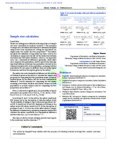
Variability Without what there is no need for statistics? The answer is variability. Variability is the most important factor in sample size calculation in case of continuous outcome. Sample size determination is based on population variance of a given outcome variable that is estimated by means of the standard deviation (SD). Generally population variance is an unknown value so the researchers use either estimate of variance from pilot study or values from literature of same kind of studies done in past. The variability of the continuous outcome measure, expressed as the SD. The greater the spread in outcome variable, it is more expected that the values will be overlapped in groups. Using most precise measurement is the only solution to get validated results. With smaller variability, smaller quantity of subjects Source: cyntegrity.com required if other factors required for sample size calculation is being fixed. The figure explains variability and spread of different kind.

Page 3 of 21


iv.

Types of Errors In concluding any kind of research, you may come across with two types of error. Table 1 illustrates the process of decision making in hypothesis testing. In columns two possible states of reality are presented i.e. null hypothesis (H0) is true in reality and H0 is false in reality. Whereas rows on the left side are shown as the two possible decisions which can be made: accepting and rejecting null hypothesis. Table 1: Decision Table in Hypothesis Testing REALITY H0 is true H0 is accepted DECISION H0 is rejected

H0 is false





Correct Decision

Type II Error





Type I Error

Correct Decision

You do not know the reality and that is why you do research. Based on your experiences and gathered information, you have to take decision; you have to conclude your research. H0 is represented as null hypothesis which is nothing but a null statement towards your assumption. Let us assume that H0 is true in reality (which is unknown) and your decision (based on the data analysis) suggests accepting H0 which will be the correct decision made by you. Likewise let us assume that H0 is false in reality (which is unknown) and your decision (based on the data analysis) suggests rejecting H0 which will be again a correct decision made by you. Now what if null hypothesis is true in reality (which is unknown) and your decision (based on the data analysis) suggests rejecting H0. Similarly what if null hypothesis is false in reality (which is unknown) and your decision (based on the data analysis) suggests accepting H0. These are the circumstances where wrong decisions have been made. These two types of circumstances are two types of errors which you might come across and called as Types of Errors in hypothesis testing. Type I Error is when null hypothesis is true in reality and a significant result is obtained (you have to reject the null hypothesis). Type II Error is when null hypothesis is false in reality and a non-significant result is found (you have to accept the null hypothesis). Probability of conducting type I error is called as alpha (), the level of significance whereas probability of making type II error is known as beta ().

Page 4 of 21


Type II error is also known as chance of missing clinically meaningful difference. v.

Power The power of a study is the ability to see the existence of treatment effect in a study. In the above section, probability of type II error is known as beta and the value of 1 – beta (1 – ) is called the power of the test. The power of the study or test increases as the difference between the hypothesized null value and real value increases. A high power study will have low chance of a type II error. In simple term, the more difference in reality and null hypothesis, the greater is the power of the test. Power is the probability of correctly rejecting a null hypothesis i.e. null hypothesis is rejected when there is certainly a real difference or association exists. Higher the power, lower the chance of missing a real effect. Adequate power for a study is generally accepted as 0.8 (80%). The higher the power (power = 1 – beta) for a study, the larger the sample size that is required. Power is typically set at 80%, 90% or 95%. Power should not be less than 80%. Generally 90% power or more is recommended to calculate sample size to achieve real effect of the experiment. It can be determined by roughly few factors such as the magnitude of the treatment effect, the sample size, alpha (the level of statistical significance required), and study duration for survival studies. Generally, power is affected by: Let us take an example with two-arm study with total sample size 32 that means 16 subjects in each arm.  Variation (2) Lower the variability, higher the power;  Significance level () Greater the level of significance, higher the power;  Difference to be identified () Higher the difference to be detected, greater the power keeping other factors constant;  Type of Hypothesis Power is greater in one-tailed hypothesis as compared to two-tailed. Let us now fix power to be 81%, difference () to be 2, variability () to be 2 and alpha to be 0.05 with two-tailed hypothesis and see power changes with change in other factors. Factors Power

Variability =1 99.99% 

=2 81%

=3 47%  Page 5 of 21


Significance level  = 0.01  = 0.05  = 0.10 81% 69%  94%  Difference to be detected =1 =2 =3 81% 29%  99%  Sample Size n = 28 n = 32 n = 64 81% 75%  98%  Hypothesis Two-tailed One-tailed 81% 88%  vi.

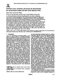
Minimum clinically relevant difference This is the minimum difference between the group means or proportions which would be considered to be clinically important. The minimum clinically relevant difference can be calculated by various methods and every method has advantages and disadvantages. Basically, the standardized difference i.e. effect size is the combination of the minimum clinically relevant difference and the variability. The standardized difference is also denoted to as the effect size and can be calculated as:

Source: Noordzij et. Al(2010)[ii]

The most accurate predictions of effect size are obtained from past and related studies involving same intervention or from their own preliminary studies or pilot work. It is also advisable to choose an effect size on expert opinion or data on the minimum clinically important difference or association. For example, Hopkins, Hawley, and Burke (1999) delimited worthwhile effect sizes for athletic performance variables on the basis of the likelihood of winning a medal at major championships. 4. Steps of calculating sample size Sample size calculation can be done at two stages i.e. at design stage and at interpretation (analysis) stage. Design Stage: At the time of planning a research, study design require the number of subjects to be studied. You need to approach an optimum number of subjects to answer your research question. Calculation of sample size basically required three things i.e. a desired power, a desired level of significance () and a clinically meaningful difference.

Page 6 of 21


Analysis Stage: Let us assume that the specific number of subjects can be obtained for my research in case of exceptional outcomes. In this case, power of the study can be calculated for a given sample size and a level of significance. 5. Sample Size Calculations It is immensely recommended that you ask a professional statistician to conduct the sample size calculation. However you may try calculating it in consultation of a statistician and with specific information. To answer the question of “How many subjects do I need for my study?”, two preliminary questions must be answered. 1. What is the study design? 2. What kind of primary outcome variable is there? What is the study design? There can be two types of study designs i.e. descriptive and comparative. Descriptive studies include cross-sectional (one time point) studies to assess prevalence, need assessments etc. with aim to estimate the rates, proportions and means in the population with secondary objective to examine whether rates are related to demographic variables such as correlation analysis. Calculation of sample size for descriptive studies is basically based on confidence intervals i.e. the precision required for estimation of rates, proportions and means. Descriptive studies have been already described in Section 3(i). On the other hand, comparative studies include case-control study, cohort study, clinical trial etc. where the key is the number of groups to be compared i.e. two or more groups. The foremost objective of this type of design is to establish whether there are statistically significant differences exist between groups with respect to primary outcome variable. Sample size calculation in comparative studies is based on hypothesis testing and power. What kind of primary outcome variable is there? Data on many variables are collected in a study other than outcome and exposure variables. Choosing a primary outcome variable and exposure depends on your research question. It is analogous to choosing party dress in a cloth shop. You may have many favorites, but you have to choose one besides that you want to try many. Research question of a study is designed in such a way that it may have one outcome variable. A quantitative variable is one where the characteristics is measured on a scale with many possible values representing a range for example age, height, blood pressure or pain (Visual Analogue Scale (VAS)). It requires a measuring instrument (ruler, biochemical analysis, weighing machine etc.) with standard unit (cm, mg/dl, kg etc.). These variables are summarized as mean or median. Discrete variable means count data or complete number which cannot be represented in decimal points e.g. number of subjects, number of visits etc. whereas continuous variable can take any value (infinite value) between two numbers and can be represented in terms of decimal points. Page 7 of 21


A qualitative variable is which cannot be measured using any instrument or cannot be represented by a standard unit. It only can be classified into one of a number of categories on the basis of characteristics of variable. Nominal variable is such where order does not matter for example gender or blood group however the ordinal variable is where order does matter for example education, pain etc. Classification can be better understood by the following diagram:

Data

Quantitative (Numerical)

Discrete

Continuous

Qualitative (Categorical)

Binary

Multiple Nominal

Ordinal

Other than this you required following information as well; which may influence sample size:  How to evaluate minimum clinically relevant difference (smallest treatment effect)? It can be identified by systematically review the literature on previous studies or by discussing trial design with experts of the field. For example, mortality rate seen in the treatment group might be 10% (it is 12% in general population) therefore, the absolute treatment effect that we are trying to detect will be 2% (12% – 10%), generally denoted by δ. 

Are there any covariates which need to be controlled? When you plan a research you gather information on various factors other than outcome and exposure. These other factors are known as covariates such as confounders, effect modifiers and interactions. It is very much required to identify these covariates (either through available literature or multivariable statistical analysis) and adjust for it when planning the study. Some of the covariates are very well known such as gender and age are considered as known confounders for many studies.

Page 8 of 21




What is the unit of randomization? Is it individual subjects, household, site, hospital wards, communities, families, etc? Randomization technique helps deciding power of the study. A cluster randomized design has lower statistical power than a subject-randomized trial of equivalent size because of observations within each cluster being correlated. A clustering measure is known as the ‘intra-cluster correlation coefficient’ (ICC). Because of this, sample sizes require to be exaggerated to adjust for the clustering effect. The cluster size and the ICC both influence the growth required. If you have cluster size above 50 then you may get little increased power, whereas researchers have to look for the costs related with recruitment of additional clusters.



What is the unit of analysis? It is individual subjects or clusters for example family practices, hospital wards, communities, families.



How long is the duration of the follow-up? Is it long enough to be of any clinical relevance? Time duration of a study is also an important factor to be considered while calculating sample size. This is useful for prospective/follow-up studies.



What is the desired level of significance ()? Section 3(iv) explains about types of errors. Alpha () is the probability of conducting type I error and Beta () is the probability of conducting type II error. Probability can be calculated by dividing total number of outcomes in favorable outcome. Here the reality is unknown as that is why denominator cannot be found to calculate these probabilities. Consequently level of significance (alpha,) has to be assumed by the researcher. These assumptions support the interpretation of result after the data analysis. If you considering 5% level of significance at the time of sample size calculation, you will be able to interpret your results with 95% confidence. You cannot interpret your result with 96% or 99% confidence. By fixing 5% level of significance you are taking type I error into account which means that there might be 5% chance of rejecting null hypothesis when it is true (you cannot neglect it). 5% level of significance also means there is up to a 5% probability of interpreting that there is signal of an effect, when in fact none exists. 1% level of significance is sometimes more appropriate, in case of avoiding conclusion that there is signal of an effect when it does not exists in reality.



What is the desired power (1 – )? It is evident from above section that you cannot calculate probability of type II error however you may have to assume it. The Power of a study or statistical test is the probability that it correctly rejects the null hypothesis (H0) when the null hypothesis is false (i.e. the probability of not committing a Type II error, or β).

Page 9 of 21


Power calculation is used when sample size is fixed which happened in rare studies. In sample size calculation, power should not be considered less than 80%. It is recommended that always try to select power 90% so that the real effect in planned study can be found. 

What is the test statistic which will be used for analysis? Will it be a one- or two-tailed test? Many software are available to calculate sample size and most of them are based on test statistic or summary. If you know one of them, you may calculate the sample size with desired level of significance and power. Whether it will be onetailed or two-tailed test, it is decided with the help of alternative hypothesis (H1). In a two-sided test, the null hypothesis states there is no effect, and the alternative hypothesis regularly implied is that a difference exists in any direction. Alternative hypothesis of a one-sided test does specify a direction, e.g. alternative hypothesis will be an active treatment is better than a placebo, and the null hypothesis will be that there is no difference between active treatment and placebo. In general two-sided tests are recommended to use unless otherwise you have strong evidence or a good reason for doing this research. In case if the true effect is in the opposite direction to that expected, this does not mean that there is no effect, and should be reported as such; a one-sided test would not allow this.

Basically there are two techniques of sample size calculation i.e. estimation and hypothesis testing. Estimating a parameter is used for single group studies whereas hypothesis technique is used for two-group study to compare to group. There are numerous ways to understand method of sample size calculation which depends on text books, software used etc. Approximately more than 100 methods are there to calculate sample size on the basis of research question, study design, parameter, statistical test etc. Scope of this book is limited so widely and frequently used methods are being discussed. 5.1 SAMPLE SIZE FOR SINGLE-GROUP STUDIES If no comparisons are involved, sample size calculation should be based on precision i.e. parameter’s confidence interval. The essence is that the required precision of estimate needs to be decided before the start of the study. It can be assumed through clinical judgement as to what would be acceptable to the scientific community. Wide confidence intervals don’t give good information. a. Estimating a single mean for a continuous outcome In case of continuous outcome variables it is assumed that continuous outcomes are plausibly sampled from a Gaussian (normal) distribution. In this situation the best summary statistics of the data is the mean. Page 10 of 21


The sample size of a study will naturally depend on the subject matter and the aims of the exercise, the desired precision etc. For each study subject various numerical measurements will be recorded; for example, age, weight, height, blood pressure, body temperature etc. In this case the data are summarized by means and variance or their derivatives. Determination of sample size has to take into account the way the outcome will be measured. Formula is based on the assumptions that the outcome variable is continuous; sampling distribution of the sample mean is approximately normal and the observations are independent. Formula

Where,  is standard deviation d is precision 1- /2 is the desired level of significance Example Calculate the sample size needed to achieve 5 mg/l plasma lamotrigine (LTG) among patients who have seizures with 1.0 mg/l precision and 95% confidence. Based on a pilot study, the standard deviation of plasma lamotrigine was 2 mg/l. In this example  = 2, d = 1.0 mg/l and Z1- /2 is the coefficient which has fixed values for specific level of significance. In this case Z1- /2 = 1.96 as significance level is 95%. If level of significance is 99% then the value of Z1- /2 will be 2.576. These values are fixed based on properties of normal distribution.

b. Estimating a single proportion or percentage for a categorical outcome A proportion is outcome of a binary variable, where for each individual in the sample gets the one value alternatively A and B. For example, survival of a patient (A) or death (B), a test is positive (A) or negative (B). The proportion (p) of survival is the number of alive cases divided by the total number in the sample. Let us understand this with one example. Suppose a doctor chooses a random sample of 215 women from the hospital records for her general practice, and finds 39 of them have a history of suffering from asthma. Then the proportion will be p = 39/215 = 0.18. The formula works on the assumption that the outcome variable should be binary (alive/dead, yes/no); if p is probability of success in each trial/study then (1-p) is probability of failure and sampling distribution of the sample proportion (p) is approximated to normal. Formula

Page 11 of 21


Where, p is the expected proportion d is absolute precision 1- /2 is the desired level of significance Example A researcher wishes to estimate the prevalence of tonsillitis among children less than five years of age in its locality. It is known that the true rate is unlikely to exceed 20%. The researcher wants to estimate the prevalence to within 5 percentage points of the true value, with 95% confidence. How many children should be included in the sample?

What if precision is not absolute? A relative precision measures how close an estimate is to the true value of sample. Precision is description of the agreement of a set of measures taken in the same manner. It relates to the confidence interval and defined in terms of repeated sampling. It will not be given in percentage points of true population. For example an investigator working for a national programme of immunization seeks to estimate the proportion of children in the country who are receiving appropriate childhood vaccinations. What will be the sample size if the resulting estimate is to fall within 10% (not 10 percentage points) of the true proportion with 95% confidence? The vaccination coverage is not expected to be below 50%. Result will be that for p = 0.50 and E = 0.10 (relative) a sample size of 384 would be needed. 5.2 SAMPLE SIZE FOR TWO-INDEPENDENT GROUP STUDIES The sample size calculation of two-independent groups depends on significance level, power and minimum difference to be detected with this power. Significance level needs to be defined whether one-tailed or two-tailed. In most of the cases it is considered to be two-tailed. a. Comparing Two Means - Estimation This procedure is useful in the calculation of the sample size when the research objective is to estimate clinically meaningful difference between means of any two independent groups. For example, an investigator wants to estimate the clinically meaningful difference between mean haemoglobin levels of males and females. The formula is based on the assumptions that outcome variable is continuous; sampling distribution of the sample mean is approximately normal; Page 12 of 21


observations are independent and the variances in the two groups are similar. If these assumptions are fulfilled then the following formula can be used to calculate sample size for two-independent groups. Formula

Where,

is pooled standard deviation is standard deviation in first group is standard deviation in second group d is the precision 1- /2 is the desired level of significance Example A study was planned to measure the difference in caloric intake at lunch between two schools, where one school received hot lunch program while the other did not. From other nutrition studies, they estimated that the standard deviation in caloric intake among elementary school children was 70 calories, and they wished to make their estimate to be within 15 calories of the true difference with 95% confidence. What is the required number of children to be studied for the above program? It is given that standard deviation in both the groups is 70 and absolute precision is 15.

= 85.38  86 So the total sample size needed will be 172. b. Comparing Two Means – Hypothesis Testing To approach a question “what is the probability that the difference on blood pressure of 4 mm Hg between treatment and control group is by chance?” It can be assumed that the difference is not due to chance, and there is a significant effect of the drug on blood pressure if this probability is small adequate. The theory of sample size calculation for this situation depends on the assumptions that the outcome variable is continuous; sampling distribution of the sample mean Page 13 of 21


is approximately normal; observations are independent and the variances in the two groups are similar. Formula

Where,

is pooled standard deviation is standard deviation in first group is standard deviation in second group is the mean difference between samples 1- /2 is the desired level of significance 1 -  is the desired power Example A randomized trial was conducted by the nutrition department to see whether a dietary supplement given to pregnant women will reduce the systolic blood pressure (SBP) level during the time of delivery. One group received the new supplement whereas the other group received the normal diet. From a pilot study, the standard deviation of SBP was 40 mm/hg and it is expected to be the same for both the groups. What is the required sample size if we expect a difference of 20 mm/hg SBP at 5% level of significance with 90% power? It is given that standard deviation in both the groups is 40 and difference in means is 20.

= 84.1  85 So the total sample size needed will be 170. There are standard values of Z1-/2 and Z1- which is given in following table for your reference:

Table 2: Standard value of coefficient of type I and type II errors Type I () Error

Type II () Error Page 14 of 21


Probability 0.05 (5% significance) 0.01 (1% significance) 0.001 (0.1% significance)

Z1-/2 1.96 2.57 3.29

Probability 0.05 (95% power) 0.10 (90% power) 0.15 (85% power) 0.20 (80% power) 0.25 (75% power)

Z1- 1.64 1.282 1.037 0.842 0.675

c. Comparing paired sample means In some studies, paired data is measured as a continuous outcome in each subject at the start (baseline) and end of the study period. Paired outcome data may have more power to detecting differences because individual variation is reduced. Another type of pairing may occur in diseases such as lungs, kidneys, and eyes are randomized to receive control therapy which may affect two organs. For this special kind of stratification, sample size calculation needs to take account for. For continuous outcomes, a mean difference in outcome between a treated and untreated eye would measure the treatment effect and could compared using a paired t-test. The formula works on assumption that outcome variable is continuous; sampling distribution of the sample observation is approximately normal and the most important is that observations are paired. Formula 

 Where,

 1- /2 is the desired level of significance 1 -  is the desired power 1 is standard deviation of baseline values 2 is standard deviation of post-treatment values  is effect size Example An investigator wants to associate the change in blood pressure before and after the administration of a drug. If the investigator is observing the difference between the pre (Mean BP=95) and post (Mean BP=85), and with the between subject Standard Deviation as 10, for a 5% error (two sided) and 90% power. How many patients should he need?

= 12.4  13 Page 15 of 21


where  d. Comparing Two Proportions – Estimation The magnitude of the difference between two population proportions is repeatedly of interest. We may want to compare, for example, men and women, two age groups, two socio economic groups, or two diagnostic groups with respect to the proportion possessing some characteristic of interest. The formula works on the assumption that outcome variable measure should be binary (yes/no, success/failure, alive/dead etc.) and the sampling distribution of the sample proportion is approximated to normal. Formula 

Where, 1- /2 is the desired level of significance p1 is proportion in first group p2 is proportion in second group d is population risk difference Example An investigator started research with, research question i.e. whether clonidine is effective in the treatment of postoperative shivering. He is specialized in anesthesiology, he finds out that the incidence of postoperative shivering is 60%. He wants to find out the effectiveness of the drug clonidine in reducing this incidence. Reduction up to 40% (i.e. from 60% to 20%) in the incidence of shivering will be clinically beneficial. How many patients should be recruited for the study with alpha value i.e. Type I error of 5% (0.05) and the power of 95%?

= 38.4  39 Investigator decides to recruit 40 individuals in each group in the study. e. Comparing Two Proportions – Hypothesis Testing This section focusses on studies designed to test the hypothesis that two population proportions are equal. For studies concerned with very small proportions. In this case where the underlying rate is very rare, the Poisson approximation can be used for comparison of proportions that fall below the Page 16 of 21


lower limit (that is, 0.05) specified for the arcsine transformation provided nP 1 and nP2 are both large (10). The formula is based on the assumption that outcome variable measure should be binary (yes/no, success/failure, alive/dead, etc.); p is probability of success in each trial; (1-p) is probability of failure; the sampling distribution of the sample proportion is approximated to normal and proportions are independent of each other with very small amount (i.e., < 0.05). Formula

Where, 1- /2 is the desired level of significance 1 -  is the desired power p1 is proportion in first group p2 is proportion in second group d is the difference in two proportion Example In an investigation two communities were identified to participate in a study to evaluate the wide scale use of new screening program for early identification of breast cancer. In one community, the screening program will be used on all women over the age of 35, while in the second community it will not be used at all. The annual incidence rate of breast cancer is 50/100,000=0.0005 in an unscreened population. A drop in the rate to 20/100,000=0.0002 would justify using the procedure on a widespread basis. How many women should be followed in each of the two communities to detect a drop in the rate this large if the hypothesis test will be performed at the 5% level of significance with a power of 80%?

= 6106.5  6107 Total number of women required for this investigation will be 12214. 6. Important Rules of Thumb 

Sample size calculation requires basically these parameters: – Difference (effect) to be detected () – Variability of an outcome (2) – Equal/ unequal group size – Significance level ()  One-tailed or two-tailed – Power Page 17 of 21


  

– Objective Effect size and error value are projected by studying research problem in depth, literature search, experts consultation in the area of interest or from a pilot study with limited number of subjects. When treatment effect is small, sample size increases for example when comparing two drugs rather than a drug versus placebo. Sample size estimation should be based upon statistics which is being used in the analysis. It should not be the case that sample size is based on continuous outcome variable and dichotomous outcome variable is used for the analysis. Because using a different statistic for analysis may alter the anticipated power and treatment effect. “There is one and only one statistical method for one objective in any research.”  Gayatri Vishwakarma

    

Round up your sample size after estimation and do not round down. Up means 10.04 becomes 11 and not 10. Get involve statistician in sample size calculation. They can add new and fresh prospective in your research. When there is high variability (known as ‘noise’) and measurements are at peak flow rate; a simple way to deal with this problem is to take a few repeated measurements and use the average or highest value of these observations. Give a thought to “What difference is scientifically important in units” i.e. 0.01 inches or 10 mm Hg in systolic blood pressure. Sample Size Adjustments: It is important to note that sample-size calculation is subjective and will vary from study to study depending on the context. The sample size may need to be adjusted to account for the effects of other variables, and the uncertainty of predictable practical and ethical factors. – When one of several primary outcomes or several pairwise comparisons is required to draw a conclusion, multiplicity adjustment using the Bonferroni method to the level of significance should be made. – The initial sample size may need to be adjusted in order to account for lost to follow-up and expected response rate. Let us assume that n is the total number of subjects in each group without accounting for loss to follow-up and L is the loss to follow-up rate, then the adjusted sample size will be: –



In case of unequal group size, after calculating n per group (assuming equal number per group), following will be the formula to calculate sample size per group:

where ratio which is required in two unequal groups. The basic formula for calculating sample size to test equality of two means is: Page 18 of 21




The basic formula for calculating sample size to test equality of two proportions is:

7. Software for Sample Size Calculations Len Thomas and Charles J. Krebs have given an informative review of some software of sample size calculation:  nQuery advisor  Power and Precision  PASS 2017  nMaster 2.0  Piface Abundantly free software are available for sample size calculation. Please be careful while using them as validation of these software are doubtful. 8. Exercise 8.1 Multiple Choice Question 1. Which of the following statements are true?  The larger the sample size, the greater the sampling error  The more categories or breakdowns you want to make in your data analysis, the larger the sample needed  The fewer categories or breakdowns you want to make in your data analysis, the larger the sample needed  As sample size decreases, so does the size of the confidence interval 2. Which of the following factors is not necessary in determining sample size?  Estimated standard deviation of the population  Magnitude of acceptable error  Confidence level  All of the above are necessary. 3. Sample size is an issue at  Design stage  Interpretation stage  Both  Not at all an issue 4. Study may fail to detect important effects or associations if  Sample size is too small  Sample size is too large  Not an issue  None of the above 5. Prerequisites for determining sample size are Page 19 of 21


6.

7.

8.

 Type of variables  Type of study design  Type I error and Type II error  All of the above ___________ is a set of elements taken from a larger population according to certain rules.  Sample  Population  Statistic  Element It is recommended to use the whole population rather than a sample when the population size is of what size?  500 or less  100 or less  1000 or less  you should always use a sample A number calculated with complete population data and quantifies a characteristic of the population is called which of the following?  A datum  A statistic  A parameter  A population

9.

Which of the following formulae is used to determine how many people to include in the original sampling?  Desired sample size/(Desired sample size + 1)  Proportion likely to respond/desired sample size  Proportion likely to respond/population size  Desired sample size/Proportion likely to respond 10. _____ is the appropriate criterion for selecting either a t-test or a Z-test regarding the difference between two groups when comparing proportions.  Value of the population standard deviation  Degrees of freedom  The coefficient of determination  Sample size  None of the above 8.2 Problems 1. Calculate the sample size to estimate Diastolic BP in a population to within ±2mmHg (using 95% CI) and the SD of DBP was known to be 15mmHg by adding 10% non-response rate. Ans: 242

Page 20 of 21


2. Suppose it is thought that there are about 28% smokers in the population and it is required to estimate the percentage of smokers to within ±3% using 95% CI. Determine sample size for given situation. Ans: 957 3. Calculate the sample size for an RCT of two-arm where population proportions in two groups are given 0.7 and 0.5 respectively with 5% level of significant and 80% power. Ans: 188 9. References: i. ii.

iii. iv. v.

vi. vii. viii. ix.

x. xi. xii. xiii.

xiv.

Hayat MJ. Understanding sample size determination in nursing research. West J Nurs Res. 2013. Aug; 35(7): 943-56. Noordzij M, Tripepi G, Dekker FW, Zoccali C, Tanck MW, Jager KJ. Sample size calculations: basic principles and common pitfalls. Nephrol Dial Transplant. 2010. Jan; 25: 1388–1393. Cooper BA, Branley P, Bulfone L et al. The Initiating Dialysis Early and Late (IDEAL) Study: study rationale and design. Perit Dial Int. 2004; 24: 176–181. Altman DG. Practical Statistics for Medical Research. 1991. Chapman and Hall, London. Colangelo KJ, Pope JE, Peschken C. The minimally important difference for patient reported outcomes in systemic lupus erythematosus including the HAQDI, pain, fatigue, and SF-36. J Rheumatol. 2009; 36:2231–2237. Armitage P, Berry G, Matthews JNS. Statistical Methods in Medical Research. 2002. 4th ed. Blackwell, Oxford. Bland JM and Altman DG. One and two sided tests of significance. 1994. British Medical Journal 309 248. Daly LE and Bourke GJ. Interpretation and uses of Medical Statistics. 2007. Blackwell Science. Fifth Edition. Hopkins, WG, Hawley, JA, Burke, LM. Design and analysis of research on sport performance enhancement. 1999. Medicine and Science in Sports and Exercise, 31, 472–485. Lwanga SK and Lemeshow S. Sample Size Determination in Health Studies – A Practical Manual. WHO Geneva 1991. Lemeshow S, Hosmer DW, Klar J, Lwanga SK. Adequacy of Sample Size in Health Studies. 1990. John Wiley and Sons. Machin D, Campbell MJ, Fayers MP and Pinal APY. Sample size tables for clinical studies. 1997. Blackwell science Ltd. Second Edition. Dhulkhed VK, Dhorigol MG, Mane R, Gogate V, and Dhulkhed P. Basic Statistical Concepts for Sample Size Estimation. 2008. Indian Journal of Anaesthesia; 52 (6):788-793. Thomas L and Krebs CJ. A Review of Statistical power analysis software. 1997. Bulletin of the Ecological Society of America. 78(2): 126-139.

Page 21 of 21

Sample Size and Power Calculation

Sample Size and Power Calculation

Suggest Documents

Sampling and Sample Size Calculation

Sample size calculation

Statistical power calculation and sample size ... - UQ eSpace