Sampling Algorithm of Order Statistics for Conditional ...

Generalized P-phased Regression Estimators with Single and Two Auxiliary Variables Farhan Hameed Punjab Higher Education Department Research Scholar, Govt. College University (GCU), Lahore, Pakistan [email protected]

Hina Khan Department of Statistics, Govt. College University (GCU), Lahore, Pakistan [email protected]

Abstract Multiphase sampling has been the concept not being utilized is estimation of ratio and regression estimator widely. In the recent study we have proposed new dimension of sampling survey of estimations by proposing two generalized p-phase regression estimators with single and two auxiliary variables for estimating population mean. The proposed estimators are the generalized p-phase cases of Hanif et al (2015) and Hanif (2007) respectively. Both the estimators from which we took motivation are now special cases of our proposed estimators. We have derived unbiasedness, expression of Mean Square Errors along with family of estimators based upon p-phased generalization. We have derived expression of MSE in such a way that these expression can be used to obtained results for every phase we desire. By conducting empirical study on proposed estimators we have shown many situation in which MSE can be reduced by increasing number of phases. Hence, our study will open new horizon in the field of multiphase sampling where a lot of challenges are waiting to be resolved by proposing new estimators for phases above 2nd phase.

Keywords: MSE, NIC, Generalized P-Phased, Auxiliary Variable. 1. Introduction Sampling survey is perhaps the oldest statistical procedure to determine the accurate and useful estimates under prevailing constraints of time and money. The regression and ratio methods of estimation are two strongest pillars of sampling survey. In ratio and regression estimation many interventions in terms of estimators with different structural and functional form have been made. Two phase and multiphase sampling are the concepts associated in estimation of population mean from finite population under different cases of availability or non- availability of auxiliary information. In the recent study we have proposed new dimension of sampling survey of estimations by proposing generalized p-phase regression estimator. The proposed estimators undertakes multiphase sampling producers for estimation. Our estimator is attempt to utilize information from phases above second phase. Not only we become able to gather maximum information about auxiliary variables, but also in many cases the Mean Square Error (MSE) is also reduced. The regression estimator have been used widely by Srivastava (1967), Walsh (1970), Reddy (1973, 74), Gupta (1978), Sahai (1979), Vos (1980) for estimation. The Classical Regression Estimator (CRE) is 𝑇1 = 𝑦̅ + 𝛽𝑦𝑥 (𝑋̅ − 𝑥̅ ) (1.1) Pak.j.stat.oper.res. Vol.XIII No.3 2017 pp661-685

Farhan Hameed, Hina Khan

Vos (1980) used weighted average of Mean Per Unit (MPU) Ratio Estimator to propose following estimator:𝑦̅ 𝑇2 = 𝛼𝑦̅ + (1 − 𝛼) 𝑋̅ (1.2) 𝑥̅ where 𝛼 is constant. The estimator (1.8.1.3) is identical to MPU estimator for   1 and is identical to RE for   0 . Das (1988) with little modification of CRE proposed following estimator: 𝑇3 = 𝑦̅ − 𝑊𝜆(𝑥̅ − 𝑋̅ )

(1.3)

For 𝑊= 1 estimator (1.3) reduces to (1.2) and for 𝑊 = 0 it reduces to MPUE. Mohanty (1967) combined Ratio Estimator with two auxiliary variables and proposed the estimator:𝑍̅ 𝑇4 = 𝑦̅ + 𝛽𝑦𝑥 (𝑋̅ − 𝑥̅ ) (1.4) 𝑧̅ The estimator (1.4) reduces to (1.1) under non-availability of Z. The estimator (1.4) was termed as Regression-In-Ratio Estimator (RIRE). Samiuddin and Hanif (2006) presented RE in single phase as:𝑇5 = 𝑦̅ + 𝛼(𝑋̅ − 𝑥̅ ) + 𝛽( 𝑍̅ − 𝑧̅)

(1.5)

Now, some of the estimators in two phase sampling presented in literature are as follows:Mohanty (1967) followed (1.4) to proposed the estimator in 2nd phase sampling with two auxiliary variables under No Information Case (NIC);𝑧̅1 𝑇6 = [𝑦̅2 + 𝑏𝑦𝑥 (𝑥̅1 − 𝑥̅ 2 )] (1.6) 𝑧̅1 Chand (1975) presented estimator in Partial Information Case (PIC):𝑦̅2 [𝑧̅ + 𝑏𝑧𝑥 (𝑋̅ − 𝑥̅1 )] 𝑇7 = 𝑧̅2 1

(1.7)

There have been numerous estimators in the literature other. Some notable references are Khaire and Srivastava (1981), Saho and Saho (1993), Upadhayaya and Singh (2001), Roy (2003), Samiuddin and Hanif (2006), Hanif et al (2010). The attempts to present RE above second phase is a new dimension in this context Hanif et al (2015) presented two estimators in three phase and four phase sampling. 𝑦̅𝐻1 = 𝑦̅3 + 𝛽1 (𝑥̅1 − 𝑥̅2 ) + 𝛽2 (𝑥̅2 − 𝑥̅3 ) (1.8) ̅𝑦𝐻2 = 𝑦̅4 + 𝛽1 (𝑥̅1 − 𝑥̅2 ) + 𝛽2 (𝑥̅2 − 𝑥̅3 ) + 𝛽3 (𝑥̅3 − 𝑥̅4 ) (1.9) The optimizing constants 𝛽1 , 𝛽2 , 𝛽3 were identical as under:𝑆𝑥𝑦 𝛽1 = 𝛽2 = 𝛽3 = 𝑆2 𝑥

662

Pak.j.stat.oper.res. Vol.XIII No.3 2017 pp661-685

Generalized P-phased Regression Estimators with Single and Two Auxiliary Variables

The corresponding MSE of (1.8) and (1.9) were 𝑀𝑆𝐸(𝑦̅𝐻1 ) = 𝜃3 𝑆𝑦2 (1 − 𝜌2 ) + 𝜃1 𝜌2 𝑆𝑦2

(1.10)

The corresponding expression of MSE of (3.7.2) is as under:𝑀𝑆𝐸(𝑦̅𝐻2 ) = 𝜃4 𝑆𝑦2 (1 − 𝜌2 ) + 𝜃1 𝜌2 𝑆𝑦2

(1.11)

Based upon the finding in third and fourth phase Hanif at el (2015) concluded that MSE will tends to increase. Earlier, Samiuddin and Hanif (2007) considered NIC to present RE in two phase sampling which was similar to structural formation of (1.8) and (1.9), but in two phase sampling with two auxiliary variables :𝑦̅𝑆𝐻 = 𝑦̅2 + 𝛼(𝑥̅1 − 𝑥̅2 ) + 𝛽(𝑧̅1 − 𝑧̅2 ) (1.12) Here, the co-efficient 𝛼 and 𝛽 were obtained through optimization of the expression of MSE. The expression of MSE of (1.12) was obtained as:2 2 2 𝑌̅ 2 𝐶𝑦2 𝜃2 (1 − 𝜌𝑥𝑦 − 𝜌𝑦𝑧 − 𝜌𝑥𝑧 + 2𝜌𝑥𝑦 𝜌𝑥𝑧 𝜌𝑦𝑧 ) 𝑀𝑆𝐸(𝑦̅𝑆𝐻 ) = [ ] (1.13) 2 2 2 1 − 𝜌𝑥𝑧 +𝜃1 (𝜌𝑥𝑦 + 𝜌𝑦𝑧 − 2𝜌𝑥𝑦 𝜌𝑥𝑧 𝜌𝑦𝑧 ) The optimizing coefficients were:𝑌̅𝐶𝑦 (𝜌𝑥𝑦 − 𝜌𝑥𝑧 𝜌𝑦𝑧 ) 𝛼= 2 ) 𝑋̅𝐶𝑦 ( 1 − 𝜌𝑥𝑧 𝑌̅𝐶𝑦 (𝜌𝑦𝑧 − 𝜌𝑥𝑧 𝜌𝑥𝑦 ) 𝛽= 2 ) 𝑍̅𝐶𝑧 ( 1 − 𝜌𝑥𝑧

(1.14) (1.15)

2. P-Phased Sampling Notations The p-phase sampling plan is just the extension of 2nd phase sampling procedure. Under such plan subsequent sub samples of sizes 𝑛1 , 𝑛2 − − − − − −𝑛𝑝 are drawn for first phase, 2nd phase up to pth phase respectively. The information on auxiliary and understudy variables will be gather in similar pattern as in two phase case. Let 𝑌𝑖 , 𝑋𝑖 and 𝑍𝑖 are variables with means 𝑌̅, 𝑋̅ and 𝑍̅ and variances 𝑆𝑦2 , 𝑆𝑥2 and 𝑆𝑧2 respectively. 𝐶𝑦 = and

𝑆𝑦 𝑌̅

, 𝐶𝑥 =

𝑆𝑥 𝑋̅

and 𝐶𝑧 =

𝑆𝑧 𝑍̅

are co-efficient of variations. Also

 xy ,  xz

 yz will represent population correlation coefficients between X & Y, X & Z and Y &

Z respectively.𝑛𝑖 , 𝑖 = 1,2, … … . . 𝑝, are subsequent sample sizes. Whereas, 𝑥̅𝑖 , 𝑦̅𝑖 and 𝑧̅𝑖 , 𝑖 = 1,2, … … . . 𝑝, represent sample means at first, second and so on phases. The Finite Population Correction Factor (FPC) in p-phase Simple Random Sampling With Out Replacement (SRWOR) sampling will be denoted by 𝜃𝑖 , 𝑖 = 1,2 … … . 𝑝, and given as:𝑁−𝑛 𝑁 𝑛 1 1 𝜃𝑖 = 𝑁𝑛 𝑖 = 𝑁𝑛 − 𝑁𝑛𝑖 = 𝑛 − 𝑁 = 𝑛𝑖−1 − 𝑁 −1 (2.1) 𝑖

𝑖

𝑖

𝑖

Also we have:𝜃𝑖 > 𝜃𝑗 for 𝑖 > 𝑗


(2.2)

663


The error term in each of the variables will be represented as under with the assumption that the quantities|𝑒̅𝑥𝑖 |, |𝑒̅𝑧𝑖 | are very small as compare to |𝑋̅| and |𝑍̅|. 𝑥̅𝑖 = 𝑋̅ + 𝑒̅𝑥𝑖 𝑧̅𝑖 = 𝑍̅ + 𝑒̅𝑧𝑖

(2.3)

𝑦̅𝑖 = 𝑌̅ + 𝑒̅𝑦𝑖 𝑖 = 1,2 … … … 𝑝}

Furthermore, the following results for expectations can be derived using (2.3) 𝐸(𝑒̅𝑥̅𝑖 ) = 𝐸(𝑥̅𝑖 − 𝑋̅ ) = 𝐸(𝑥̅𝑖 ) − 𝐸(𝑋̅ ) = 𝑋̅ − 𝑋̅ = 0 𝐸(𝑒̅𝑧̅𝑖 ) = 𝐸(𝑧̅𝑖 − 𝑍̅ ) = 𝐸(𝑧̅𝑖 ) − 𝐸(𝑍̅ ) = 𝑍̅ − 𝑍̅ = 0 𝐸(𝑒̅𝑦̅ ) = 𝐸(𝑦̅𝑖 − 𝑌̅ ) = 𝐸(𝑦̅𝑖 ) − 𝐸(𝑌̅ ) = 𝑌̅ − 𝑌̅ = 0

(2.4)

𝑖

𝑖 = 1,2,3 … … . 𝑝

}

The expectation of square of error terms will be as under:𝐸(𝑒̅𝑥𝑖 )2 = 𝐸(𝑥̅𝑖 − 𝑋̅ )2 = 𝜃𝑖 𝑆𝑥2 = 𝜃𝑖 𝑋̅ 2 𝐶𝑥2 𝐸(𝑒̅𝑧𝑖 )2 = 𝐸(𝑧̅𝑖 − 𝑍̅ )2 = 𝜃𝑖 𝑆𝑧2 = 𝜃𝑖 𝑍̅ 2 𝐶𝑧2

(2.5)

𝐸(𝑒̅𝑦𝑖 )2 = 𝐸(𝑦̅𝑖 − 𝑌̅ )2 = 𝜃𝑖 𝑆𝑦2 = 𝜃𝑖 𝑌̅ 2 𝐶𝑧2 𝑖 = 1,2,3 … … . 𝑝

}

In addition to (2.4) and (2.5) the following results of expectations from cross products will also be utilized:𝐸(𝑒̅𝑥𝑖 . 𝑒̅𝑥𝑗 ) = 𝜃𝑖 𝑋̅ 2 𝐶𝑥2 𝐸(𝑒̅𝑧𝑖 . 𝑒̅𝑧𝑗 ) = 𝜃𝑖 𝑋̅ 2 𝐶𝑧2 𝐸(𝑒̅𝑦𝑖 . 𝑒̅𝑦𝑗 ) = 𝜃𝑖 𝑋̅ 2 𝐶𝑦2 𝐸(𝑒̅𝑥𝑖 . 𝑒̅𝑧𝑗 ) = 𝜃𝑖 𝑆𝑥𝑧 = 𝜃𝑖 𝑋̅ 𝑍̅ 𝜌𝑥𝑧 𝐶𝑥 𝐶𝑧

(2.6)

𝐸(𝑒̅𝑥𝑖 . 𝑒̅𝑦𝑗 ) = 𝜃𝑖 𝑆𝑥𝑦 = 𝜃𝑖 𝑋̅ 𝑌̅ 𝜌𝑥𝑦 𝐶𝑥 𝐶𝑦 𝐸(𝑒̅𝑧𝑖 . 𝑒̅𝑦𝑗 ) = 𝜃𝑖 𝑆𝑦𝑧 = 𝜃𝑖 𝑍̅ 𝑌̅ 𝜌𝑧𝑦 𝐶𝑧 𝐶𝑦 𝑖 ≤ 𝑗,

𝑖 = 1,2,3 − − − 𝑝

}

Finally, the following results will also be used:𝐸(𝑒̅𝑥𝑖 − 𝑒̅𝑥𝑗 )2 = (𝜃𝑗 − 𝜃𝑖 )𝑋̅ 2 𝐶𝑥2 𝐸(𝑒̅𝑧𝑖 − 𝑒̅𝑧𝑗 )2 = (𝜃𝑗 − 𝜃𝑖 )𝑍̅ 2 𝐶𝑧2 𝐸(𝑒̅𝑥𝑖 − 𝑒̅𝑥𝑖+1 )𝑒̅𝑦𝑝 = (𝜃𝑖 − 𝜃𝑖+1 )𝑆𝑥𝑦 = (𝜃𝑖 − 𝜃𝑖+1 )𝑋̅ 𝑌̅ 𝜌𝑥𝑦 𝐶𝑥 𝐶𝑦

(2.7)

𝐸(𝑒̅𝑧𝑖 − 𝑒̅𝑧𝑖+1 )𝑒̅𝑦𝑝 = (𝜃𝑖 − 𝜃𝑖+1 )𝑆𝑧𝑦 = (𝜃𝑖 − 𝜃𝑖+1 )𝑍̅ 𝑌̅ 𝜌𝑧𝑦 𝐶𝑧 𝐶𝑦 𝑖 < 𝑗, 664

𝑖 = 1,2, − − −𝑝

}



3.

Proposed Estimators

We took motivation from Hanif et al (2015) and Samiuddin and Hanif (2006) to present estimators in generalized p-phased estimators as under. Generalizing Hanif et al (2015) estimators (1.8) and (1.9) we propose. (a)- Proposed Estimator-I Taking Motivation from Hanif et al (2015), we propose the following generalized pphased regression estimator with single auxiliary variable. 𝑝−1

𝑦̅𝐹1 = 𝑦̅𝑝 + ∑ 𝛽𝑖 (𝑥̅𝑖 − 𝑥̅𝑖 +1 ) 𝑖=1

}

(3.1)

𝑝≥2 (b)

Proposed Estimator-II

Similarly, the Samiuddin and Hanif (2006) estimator presented in (1.12) is p-phased generalized as:𝑝−1

𝑝−1

𝑦̅𝐹2 = 𝑦̅𝑝 + ∑ 𝛼𝑖 (𝑥̅𝑖 − 𝑥̅𝑖+1 ) + ∑ 𝛽𝑖 (𝑧̅𝑖 − 𝑧̅𝑖+1 ) } 𝑖=1

𝑖=1

(3.2)

𝑝≥2 4.

Unbiasedness and MSE of proposed Estimator-I

Now, we will prove unbiasedness of the proposed estimators (3.1) and (3.2) as well as the expression of MSE will be derived. Considering (3.1) and using comment (2.3) we get: 𝑝−1

𝑦̅𝐹1 − 𝑌̅ = 𝑒̅𝑦𝑝 + ∑ 𝛽𝑖 (𝑒̅𝑥𝑖 − 𝑒̅𝑥𝑖+1 )

(4.1)

𝑖=1

Applying expectation and using (2.4) we obtained:𝐸(𝑦̅𝐹1 ) − 𝑌̅ = 0 𝐸(𝑦̅𝐹 ) = 𝑌̅

(4.2)

1

From (4.2) we observed that (3.1) is unbiased estimator of Population Mean. Now, to derive MSE of (3.1) consider (4.1) and squaring both sides and applying expectations 𝑝−1 2

𝐸 [(𝑦̅𝐹1 − 𝑌̅ ) ] = 𝐸 [(𝑒̅𝑦𝑝 ) ] + 𝐸 2

[∑ 𝛽𝑖2

𝑝−1 2

(𝑒̅𝑥𝑖 − 𝑒̅𝑥𝑖+1 ) + 2 ∑ 𝛽𝑖 𝛽𝑗 (𝑒̅𝑥𝑖 − 𝑒̅𝑥𝑖+1 ) (𝑒̅𝑥𝑗 − 𝑒̅𝑥𝑗+1 ) ]

𝑖=1

𝑖 0, 𝜌𝑦𝑧 < 0

48.0557

-0.4406

0.80354

-0.3547

1678

2

𝜌𝑥𝑦 > 0, 𝜌𝑥𝑧 > 0, 𝜌𝑦𝑧 > 0

48.0557

0.4406

0.80354

0.3547

1678

3

𝜌𝑥𝑦 < 0, 𝜌𝑥𝑧 < 0, 𝜌𝑦𝑧 < 0

48.0557

-0.4406

-0.80354

-0.3547

1678

4

𝜌𝑥𝑦 > 0, 𝜌𝑥𝑧 > 0, 𝜌𝑦𝑧 < 0

48.0557

0.4406

0.80354

-0.3547

1678

5

𝜌𝑥𝑦 < 0, 𝜌𝑥𝑧 < 0, 𝜌𝑦𝑧 > 0

48.0557

-0.4406

-0.80354

0.3547

1678

6

𝜌𝑥𝑦 > 0, 𝜌𝑥𝑧 < 0, 𝜌𝑦𝑧 < 0

48.0557

0.4406

-0.80354

-0.3547

1678

7

𝜌𝑥𝑦 < 0, 𝜌𝑥𝑧 > 0, 𝜌𝑦𝑧 > 0

48.0557

-0.4406

0.80354

0.3547

1678

8

𝜌𝑥𝑦 > 0, 𝜌𝑥𝑧 < 0, 𝜌𝑦𝑧 > 0

48.0557

0.4406

-0.80354

0.3547

1678

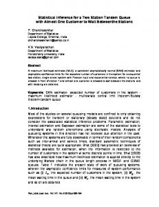
With combinations in Table 5.2.1 the MSE results are reported in Table 5.2.2. By observing results of MSE we can see only two type of results. Therefore, just two cases:(i)-All correlations are positive or two out of three correlations are negative. (ii)-All correlations are negative or two out of three are positive are produced. Now, conversing over the results in first case, MSE tends to increase slowly till phase 7. Afterwards, it has a sharp upward slop. For the seconds case MSE decreases steadily up to phase 6 and at phase 7 it is almost zero. We also observed that MSE produced are negative. This phenomenon is not the contradiction because, we have used population parameters to find values of MSE. The population parameters are constants whereas, FPC is variable depend upon phases. So, there is likelihood that MSE can be negative. Therefore, producing negative MSE is not objectionable. The graphical pattern of both cases is under Figure 5.2.1. It is evident that for case (ii) MSE is reduced while phases increased.

676



̅𝑭𝟐(𝒑) ) at Combinations of Low-Moderate Correlation Table 5.2.2: 𝑴𝑺𝑬(𝒚 Sample Size Phase S.N#1 S.N#2

̅ 𝑴𝑺𝑬(𝑦 𝐹

S.N#3

S.N#4

2(𝑝)

)

S.N#5 S.N#6

S.N#7

S.N#8

200

2

11.20

11.20

9.38

9.38

11.20

11.20

9.38

9.38

180

3

12.49

12.49

8.40

8.40

12.49

12.49

8.40

8.40

160

4

14.15

14.15

7.14

7.14

14.15

14.15

7.14

7.14

140

5

16.37

16.37

5.46

5.46

16.37

16.37

5.46

5.46

120

6

19.47

19.47

3.10

3.10

19.47

19.47

3.10

3.10

100

7

24.12

24.12

-0.42

-0.42

24.12

24.12

-0.42

-0.42

80

8

31.88

31.88

-6.31

-6.31

31.88

31.88

-6.31

-6.31

60

9

47.38

47.38

-18.09

-18.09

47.38

47.38

-18.09

-18.09

40

10

93.91

93.91

-53.41

-53.41

93.91

93.91

-53.41

-53.41

̅𝑭𝟐(𝒑) ) at Combinations of Low-Moderate Correlation Figure 5.2.1: 𝑴𝑺𝑬(𝒚

As we have just shown that only two types of results can be produced for all eight combinations of correlations therefore, in Table 5.2.3 we present intra-phase and second phased reference relative efficiencies


677


Table 5.2.3: Intra-Phase Relative Correlations Phase

MSE(Case1 )

MSE(Case2 )

2 3 4 5 6 7 8 9 10

11.2 12.49 14.15 16.37 19.47 24.12 31.88 47.38 93.91

9.38 8.4 7.14 5.46 3.1 -0.42 -6.31 -18.09 -53.41

Efficiency

of

̅𝑭𝟐(𝒑) 𝒚

Each phase/2nd phase (%) Case1 Case2 111.52 89.55 126.34 76.12 146.16 58.21 173.84 33.05 215.36 -4.48 284.64 -67.27 423.04 -192.86 838.48 -569.40

at

Moderate-Level

Each Phase / Previous Phase (%) Case1 Case2 111.52 89.55 113.29 85.00 115.69 76.47 118.94 56.78 123.88 -13.55 132.17 1502.38 148.62 286.69 198.21 295.25

For case one when see that all the reported figures are above 100 which means that there is increasing pattern in MSE. The efficiency of the estimator reduces as phase increase. But there is not a much of difference as we move from one phase to another. For case 2 both types of efficiencies are less than 100 up to phase four. Having relative efficiency less than 100 means that the performance of the estimator is getting better and better with the increment in the phase. For example if we consider phase four in 2nd case the relative efficiency for current phase versus 2nd phase is 33.05 which means MSE at phase four is just 33% of MSE which was produced by phase two. Similarly, the intra-phase efficiency for case two is also better as with increasing phase MSE decreases resulting in better performance. Now, we consider high correlation between variables and will observe what pattern MSE will display. For this purpose we will now consider only two combinations i.e. all positives and all negatives. Consider the following table 5.2.4 Table 5.2.4: Combinations of High Levels of Correlation S.N 1

2

3

4

678

Combinations of Correlation High positive between understudy and auxiliaries Low positive between auxiliaries High positive between understudy and auxiliaries high positive between auxiliaries High negative between understudy and auxiliaries Low negative between auxiliaries High negative between understudy and auxiliaries High negative between auxiliaries

̅ 𝒀

𝝆𝒙𝒚

𝝆𝒙𝒛

𝝆𝒚𝒛

N

48.0557

0.9406

0.20354

0.9547

1678

48.0557

0.9406

0.90354

0.9547

1678

48.0557

-0.9406

-0.20354

-0.9547

1678

48.0557

-0.9406

-0.90354

-0.9547

1678



We have consider four different combinations on the basic of degree of correlation between auxiliary variables. Each of high positive and high negative correlation between understudy and auxiliary variables is combined with corresponding high and low correlation between auxiliaries. One the ground of four cases we computed MSE of proposed estimator which are presented in Table 5.2.5. From the Table 5.2.5 we can observe for combinations of correlation at serial no 1 in Table 7.2.4, the MSE has shown decreasing pattern with the increase in the phase. Up to phase 7 MSE has become very low. Similarly, for combinations of serial no 3 the MSE has shown decline via increases in phases. Comparatively, for Serial no 3 the decrease in MSE is rapid than the decrease in MSE of serial no 3. For, serial number 2 the MSE almost remains constant intra-phase. After each phase there is a very minor increase MSE. For serial number 4 MSE starts from negative values. Again it is not suspicious as we have used population quantities to find MSE. If we wise to make comparison we can use magnitude of MSE in such case. ̅𝑭𝟐(𝒑) ) at Combinations of High Correlation Table 5.2.5: 𝑴𝑺𝑬(𝒚 Sample Size

̅ M𝑺𝑬(𝑦 𝐹

Phase S.N#1

2(𝑝)

)

S.N#2

S.N#3

S.N#4

200

2

9.53

10.26

8.56

-12.42

180

3

8.74

10.33

6.54

-40.67

160

4

7.73

10.44

3.95

-76.98

140

5

6.37

10.59

0.5

-125.4

120

6

4.48

10.81

-4.32

-193.1

100

7

1.64

11.13

-11.5

-294.8

80

8

-3.09

11.66

-23.6

-464.3

60

9

-12.5

12.72

-47.7

-803.2

40

10

-41

15.92

-120.2

-1820.1

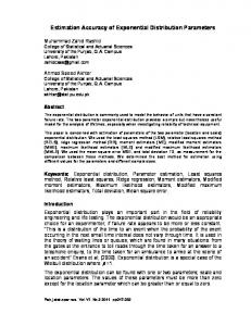
The pattern of M𝑆𝐸(𝑦̅𝐹6(𝑝) ) for all serial numbers 1 to 4 is presented graphically in figure 7.2.2. We observed that for serial number 1 and 3 MSE is showing decreasing pattern while for serial number 2 we have upward trend but it is not so sharp. By observing the numerical results and graphical pattern of MSE we can conclude that the proposed estimator will give better performance with the increasing phase when there is combination of correlations is like serial number 1, 3as mentioned in table 7.2.4


679


̅𝑭𝟐(𝒑) ) at Combinations of High Correlation Figure 5.2.2: Behavior of 𝑴𝑺𝑬(𝒚

̅𝑭𝟐(𝒑) at Combinations of High Correlations Table 5.2.6: Relative Efficiency of 𝒚 Phase 3 4 5 6 7 8 9 10

680

Each phase/2nd phase(%) S.N 1 S.N 2 S.N 3 S.N 4 91.71 100.68 76.40 327.46 81.11 101.75 46.14 619.81 66.84 103.22 5.84 1009.66 47.01 105.36 -50.47 1554.75 17.21 108.48 -134.35 2373.59 -32.42 113.65 -275.70 3738.33 -131.16 123.98 -557.24 6466.99 -430.22 155.17 -1404.2 14654.59

Each phase/Previous phase(%) S.N 1 S.N 2 S.N 3 S.N 4 91.71 100.68 76.40 327.46 88.44 101.06 60.40 189.28 82.41 101.44 12.66 162.90 70.33 102.08 -864.0 153.99 36.61 102.96 266.20 152.67 -188.41 104.76 205.22 157.50 404.53 109.09 202.12 172.99 328.00 125.16 251.99 226.61



Table 5.2.6 presents measures of relative efficiency for combinations of high correlations presents in table 5.2.6. For combinations at serial number 1 and 3 both the measures of efficiencies are less than 100 up to phase five and phase four respectively and afterwards they becomes negative. This means that performance of proposed estimator will get better and better with increase in number of phase where there is combinations of correlations at serial number 1 and 3 in table 5.2.4. For serial number 2 the measures are boarding little above 100. It can be interpreted that MSE will not differ to large extend with increasing number of phases. For serial number 4 since the MSE starts with negative values and kept on increasing in terms of magnitude so we conclude from this evidence that the combinations at serial number 4 in table 5.2.4 are not suitable for our proposed estimator. As a final comment we say that in case we have combinations of high correlations in such a way that high positive or high negative correlation between understudy and auxiliaries combined with low positive or negative correlations between auxiliaries and our proposed estimator will produce better results with increasing phase. After discussing performance of proposed estimator (3.2) at combinations of high correlations. Now, we will examine its performance at low correlations. For this task consider table 5.2.7. Table 5.2.7: Combinations of Low Levels of Correlation S.N

Combinations of Correlation

̅ 𝒀

𝝆𝒙𝒚

1

Low positive between understudy and auxiliaries Low positive between auxiliaries

48.0557

0.2406

2

Low positive between understudy and auxiliaries high positive between auxiliaries

48.0557

3

Low negative between understudy and auxiliaries Low negative between auxiliaries

4

High negative between understudy and auxiliaries High negative between auxiliaries

𝝆𝒚𝒛

N

0.20354

0.2547

1678

0.2406

0.90354

0.2547

1678

48.0557

-0.2406

-0.20354

-0.2547

1678

48.0557

-0.2406

-0.90354

-0.2547

1678


𝝆𝒙𝒛

681


̅𝑭𝟐(𝒑) ) at Combinations of Low Correlation Table 7.2.8: 𝑴𝑺𝑬(𝒚 Sample Size 200 180 160 140 120 100 80 60 40

M𝑺𝑬(𝑦̅𝐹2(𝑝) ) Phase S.N#1 S.N#2 S.N#3 2 11.32 11.37 11.26 3 12.76 12.87 12.61 14.61 14.80 14.36 4 5 17.08 17.36 16.68 20.54 20.96 19.94 6 7 25.72 26.36 24.82 34.36 35.35 32.96 8 9 51.64 53.33 49.24 10 103.49 107.29 98.08

S.N#4 9.82 9.39 8.83 8.08 7.04 5.47 2.87 -2.35 -18.01

̅𝑭𝟐(𝒑) ) at Combinations of Low Correlation Figure 5.2.3: Behavior of 𝑴𝑺𝑬(𝒚

682



For combinations of low level correlations presented in table 5.2.7 the results of MSE of proposed estimator (3.2) are presented in table 5.2.8. The corresponding graphical representation is in figure 5.2.3. From table 5.2.8 we observed that MSE of the estimator tends to increase for first three combinations of low level correlations. The incremental rate in all first three case is almost same. Also there is not a rapid uplift in MSE for all three cases. For fourth combination of correlations at low levels, MSE has the decreasing trend. The MSE shows continuous decrease up to phase 8. The graphical pattern of MSE of the results produced in table 5.2.8 shows upward slopes of first three combinations. The slope for fourth combination is downwards which testify that MSE has a decreasing trend. Table 5.2.9 is demonstration of relative efficiency according to all four combinations in Table 5.2.7. We observed that for first three combination both type of efficiencies are more than hundred. Which means that with increasing phase the relative efficiency of the estimator decline. Whereas, for the fourth combination the relative efficiencies are less than 100. In fact with the increase in phases the MSE rapidly decline and performance of the estimator gets better and better. ̅𝑭𝟐(𝒑) at Combinations of Low Correlations Table 5.2.9: Relative Efficiency of 𝒚 Phase

6.

Each phase/2nd phase(%)

Each phase/Previous phase(%)

3

S.N 1 112.72

S.N 2 113.18

S.N 3 112.05

S.N 4 95.57

S.N 1 112.72

S.N 2 113.18

S.N 3 112.05

S.N 4 95.57

4

129.07

130.13

127.55

89.88

114.51

114.97

113.83

94.04

5

150.87

152.73

148.21

82.29

116.89

117.37

116.20

91.56

6

181.40

184.36

177.14

71.67

120.23

120.71

119.52

87.09

7

227.19

231.82

220.53

55.73

125.24

125.74

124.49

77.76

8

303.50

310.91

292.84

29.17

133.59

134.12

132.79

52.34

9

456.12

469.10

437.47

-23.96

150.29

150.88

149.39

-82.13

10

913.99

943.65

871.36

-183.33

200.38

201.16

199.18

765.26

Conclusions and Recommendations

On the grounds of mathematical results, mathematical comparisons, constructed families and empirical studies of proposed estimators (3.1) and (3.2) we can draw following conclusions 1.

Our proposed Estimators are generalized p-phased which provide flexibility to go up to any phase of sampling. Furthermore, for every desired phase we do not have to construct mathematical expressions right from the word go. We have readymade expressions of MSE and just need to replace desired value of 𝑝.


683


2.

The proposed estimator-I is generalized p-phased and estimators by Hanif et al (2015) are now special cases of the proposed estimators-I, for 𝑝 = 3 and 𝑝 = 4 respectively.

3.

The proposed estimator-II is also generalized p-phased and estimators by Samiuddin and Hanif (2007), Hanif et al (2015) and proposed estimator-I are now special cases of the proposed estimators-II, for different conditions over 𝑝, 𝛼𝑖 and 𝛽𝑖 .

4.

Based upon the results of empirical study conducted for proposed estimator-I we can conclude that the MSE of the estimator will have increasing tend with increasing phases. This conclusion is based upon generalized results in contrast to the same conclusion drawn by Hanif et al (2015), who just utilized third and fourth phase.

5.

In case of large population we observed that MSE of (3.1) are very close to each other. Therefore, the loss in efficiency will be negligible if we wish to go beyond 2nd phase. In this way we can get maximum information out of samples as well as the desired principal of repetition can also be achieved under NIC.

6.

The empirical study for proposed estimator-II reviled that for all possible eight combinations of correlations between variables only two types of results of MSE are produced. This is because of the structural formulation of the expression of MSE of (3.2) presented in (5.1.27).

7.

̅𝑭𝟐 ) is anti. For For moderate-low correlation in both cases the behavior of 𝑀𝑆𝐸(𝒚 ̅𝑭𝟐 ) tends to increase with number of phases. For 2nd case all positive case 𝑀𝑆𝐸(𝒚 ̅𝑭𝟐 ) has decreasing pattern. Hence, we can concluded that estimator (3.2) 𝑀𝑆𝐸(𝒚 will be useful under the situation of case (ii). It will not only reduce MSE but also the efficiency of the estimation will also be enhanced.

8.

For other different combinations of correlations we may conclude that estimator (3.2) will perform better by reducing MSE and increasing efficiency when there is (i)-High positive correlation between 𝑦 and 𝑥 , 𝑦 and 𝑧 and low positive between 𝑧 and 𝑥. (ii)-High positive correlation between 𝑦 and 𝑥, 𝑦 and 𝑧 and low negative between 𝑧 and 𝑥. (iii)-High negative correlation between 𝑦 and 𝑥, 𝑦 and 𝑧 and low positive between 𝑧 and 𝑥. In all other case there is a smooth steady and slow increase in MSE per phase.

References 1.

Adhvaryu, D., Gupta, P.C. (1983). On some alternative sampling strategies using auxiliary information. Metrika, 30, 4, 217-226.

2.

Chand, L. (1975). Some ratio type estimators based on two or more auxiliary variables. Unpublished Ph.D. thesis, Iowa State University, Ames, Iowa (USA).

3.

Gupta, P. C. (1978). On some quadratic and higher degree ratio and product estimators.

4.

Hanif, M., Hamad, N. and Shahbaz, M. Q. (2010) Some New Regression Types Estimators in Two Phase Sampling, World App. Sci. J., Vol. 8(7), 799–803.

684



5.

Hanif .S, Butt. N. S and Shahbaz. M. Q. (2015). On estimation in three and four phase sampling. Sci.Int (Lahore), 27(3), 2575-2578.

6.

Khare, B.B. and Srivastava, S.R. (1981). A general regression ratio estimator for the population mean using two auxiliary variables. Aligarh Journal of Statistics, 1, 43-51.

7.

Kiregyera, B. (1984). A Regression-Type Estimator using two Auxiliary Variables and Model of Double sampling from Finite Populations. Metrika. 31, 215-226.

8.

Mohanty, S. (1967). Combination of Regression and Ratio Estimate. Jour. Ind. Statist. Asso., 5,16-19.

9.

Sahai, A. (1979). An efficient variant of the product and ratio estimator. Statist. Neerlandica, 33, 27-35.

10.

Samiuddin, M. and Hanif, M. (2006). Estimation in two phase sampling with complete and incomplete information. Proc. 8th Islamic Countries Conference on Statistical Sciences. 13, 479-495.

11.

Sahoo, J. and Sahoo, L.N. (1993). A class of estimators in two-phase sampling using two auxiliary variables. J. Ind. Soc. Agri. Statist., 31, 107-114.

12.

Sahoo, J. and Sahoo, L.N. (1994). On the efficiency of four chain-type estimators in two phase sampling under a model. Statistics, 25, 361-366.

13.

Singh, H.P and Tailor. R,” Use of correlation coefficient in estimating the finite population mean”, Statistics in Transition.Vol.6(4),Pp.555-560,2003

14.

Sisodia, B.V.S and Dwivedi, V.K “A modified ratio estimator using coefficient of variation of auxiliary variable”, Jour.Ind.Soc.Agri.Stat., Vol.33(1), Pp.13-18, 1981.

15.

Srivastava, S.K. (1966). On ratio and linear regression method of estimation with several auxiliary variables. J. Ind. Statist. Assoc., 4, 66-72.

16.

Srivastava, S.K. (1967). An estimator using auxiliary information in sample surveys. Calcutta Statistical Association Bulletin, 16, 121-132.

17.

Vos, J.W.E. (1980). Mixing of direct ratio and product method estimators. Statist. Neerlandica, 34, 209-218.

18.

Walsh, J. E. (1970). Generalization of ratio estimate for population total. Sankhya, (A), 32, č. 1, s. 99 – 106.


685

Sampling Algorithm of Order Statistics for Conditional ...

Sampling Algorithm of Order Statistics for Conditional ...

Suggest Documents