between SI and SD is defined as Satellite Independent â. Service Access Points ... Correction (FEC) redundancy applied at the physical layer. The reduction is ...
Loss and Delay QoS Mapping Control for Satellite Systems Mario Marchese, Maurizio Mongelli DIST - Department of Communication, Computer and System Sciences University of Genoa, Via Opera Pia 13, 16145, Genoa, (Italy) e-mails: { Mario.Marchese, Maurizio.Mongelli }@unige.it Abstract—An optimization problem for QoS mapping over protocol layers is formalized in this work by taking the ETSI Satellite Independent-Service Access Point (SI-SAP) as technological reference. The joint optimization of loss and delay performance metrics, together with the presence of SI-SAP QoS mapping operations, introduces the generalization of the regular concept of Equivalent bandwidth. This leads to the study of a proper measurement-based control, able to capture the most stringent QoS requirement over time (between loss and delay) and the related instantaneous bandwidth need at the lower layer of the protocol stack. The control methodology is tested through real fading and traffic traces to highlight its effectiveness for real time control of QoS mapping operations. Keywords—Satellite QoS Architectures, QoS Mapping, Measurement-based control, Infinitesimal Perturbation Analysis.
I.
INTRODUCTION
QoS over telecommunication networks depends End-to-end on the QoS achieved at each layer of the network and it is
based on functions performed at the layer interfaces. ETSIBSM (Broadband Satellite Multimedia) architecture (defined in technical reports [1]) is a good example and it is the reference of this paper, which concerns satellite networks. The considered protocol stack separates the layers between Satellite Dependent (SD) and Satellite Independent (SI). The interface between SI and SD is defined as Satellite Independent – Service Access Points (SI-SAPs). QoS requirements must flow through SI-SAPs and be implemented at SD layers.
The remainder of the paper is organized as follows. The next section introduces the technological elements generating the QoS mapping problem of BSM technology. Section III reports the formalization of the problem. Section IV contains the optimized control for the joint of loss and delay constraints when QoS mapping operations are performed. Performance analysis is proposed in section V. Conclusions and future work are reported in section VI. II. QOS MAPPING OVER BSM TECHNOLOGY The QoS mapping components over BSM technology are briefly summarized. 1) Change of information unit. It is the consequence of IP traffic transport over a BSM SD portion that implements a specific technology, e.g., ATM as often done in industrial systems [3], or DVB. 2) Heterogeneous traffic aggregation. The due association of IP QoS classes to SD transfer capabilities is limited by hardware implementation constraints. A queue model describing the QoS mapping operation at the SI-SAP interface, similarly used in reference [4], is reported in Fig. 1, for DiffServ over ATM. The problem is how much bandwidth must be assigned to each SD queue so that the SI IP-based SLA (Service Level Agreement, i.e. the performance expected) is guaranteed. IP t ra f fic IP P a c k e t C la ss ifie r
EF
Some issues are topical when traffic is forwarded from SI to SD: the change of encapsulation format, the possible need of aggregating traffic with heterogeneous performance requirements and satellite channel fading. On one hand, there is the strong need that SD layers provide a service to the SI layers, but, on the other hand, it should be done with the minimum information SD-SI bi-directional exchange, which, ideally, should be limited to the performance requirement and its matching or not. The problem is therefore connected to automatic bandwidth adaptation. SD layer needs to compute on line the bandwidth to be assigned at SD buffer (i.e., the service rate) so that the performance requirements fixed by SI layers can be satisfied. In this perspective, the paper proposes a novel control scheme for the optimization of the bandwidth provision at the SD layer. It generalizes the optimization model and the results presented in [2]. Multiple traffic classes implemented at SI layer and aggregated at SD layer are considered here, along with the joint performance metric composed of packet loss probability and average delay.
A F1
A F2
AF3
AF4
BE
AA L5
A TM M A C E F q u eu e
ATM M AC AF queue
A TM M AC B E q u eu e
Figure 1. SI-SAP interface: SI (DiffServ) over SD (ATM) [1, 3, 4].
3) Fading. Let θ SD (t ) be the service rate assigned to a traffic buffer at the SD layer at time t . The effect of fading is modeled as a reduction of the bandwidth actually “seen” by the buffer [5], due, e.g., to the application of Forward Error Correction (FEC) redundancy applied at the physical layer. The reduction is represented by a stochastic process φ (t ) . At time t , the “real” service rate θˆSD (t ) (available for data transfer) is thus obtained as:
θˆSD (t ) = θ SD (t ) ⋅ φ (t ); φ (t ) ∈ [0,1]
1-4244-0357-X/06/$20.00 ©2006 IEEE
This full text paper was peer reviewed at the direction of IEEE Communications Society subject matter experts for publication in the IEEE GLOBECOM 2006 proceedings.
(1)
III.
THE SI-SAP QOS MAPPING PROBLEM
the packets belonging to a specific flow (i.e., α iSI (t ) for a
A. Stochastic fluid model and optimization problem IP Packet Loss Probability (PLP) and IP Packet Average Delay (AD) are the chosen SLA performance metrics. The mathematical framework is based on Stochastic Fluid Models (SFM) [6] of the SI-SAP traffic buffers. N SI queues and, without loss of generality, one single SD queue are considered for the analytical formulation (Fig. 2). α 1S I (t )
x1SI (⋅, t )
θ 1SI (t ) β 1SI (t )
γ 1SI (⋅, t ) α iSI
(t )
α
SI
θ
(t )
SD
LW −Thr (t ) , for PLP and AD, respectively. Concerning this issue, the paper proposes two alternatives, reported below:
(t )
SD 1) SLA reference thresholds. i LVSD (⋅) and i LW (⋅) chase threshold values that flow from SI to SD layer and are representative of the SLA PLPi* and ADi* of the i-th traffic class:
β iSI (t ) SD
SI α NSI (t ) x N ( ⋅, t )
θ NSI (t ) β NSI (t )
γ NSI (⋅, t )
The key idea is to “equalize” the QoS measured at the SD layer in dependence of the QoS imposed by the SI layer. To capture this concept, it is useful to think at a “penalty cost function”, whose values can be interpreted as an indication about the current inability of the SD layer to guarantee the SD required QoS. In practice, i LVSD (⋅) and i LW (⋅) chase the dynamic variations of the quantities (representative of the SI layer requests) identified in the following as i LV −Thr (t ) and i
x iSI ( ⋅, t ) θ iSI (t )
γ iSI (⋅, t )
given i ) within an aggregated trunk (i.e., α SD (t ) ).
SI-SAP
SI
i
LV −Thr (t ) = PLPi* ⋅ ∫
k +1
k
Figure 2. Stochastic processes and buffer set.
α iSI
i
βiSI (t )
Let (t ) and be, respectively, the inflow and outflow rate processes of the i-th traffic buffer at SI layer at time t , i = 1,..., N . The service rate of buffer i is θ iSI (t ) . It is straightforward that: SI α (t ), if xi (⋅, t ) = 0 βiSI (t ) = i SI θ i (t ), if xi (⋅, t ) ≠ 0
The
i SD LV (α SD (t ), θ SD (t ) ⋅ φ (t ))
quantities
and
i SD LW (α SD (t ), θ SD (t ) ⋅ φ (t ))
define the loss volume and the buffer cumulative workload of the i-th traffic class within the SD buffer. They are functions of the following elements: the SD inflow process α SD (t ) (deriving from the aggregation of
α iSI
(t ) , i = 1,..., N , encapsulated in a the SI inflow processes specific transport technology), the fading process φ (t ) , and the SD SD bandwidth allocation θ SD (t ) . i LVSD (⋅) and i LW (⋅) allow capturing the performance level of each traffic class i for PLP and AD, respectively. It is worth noting that no analytical expression for them is available, since there are no instruments for the mathematical description of the statistical behavior of
(3)
LW −Thr (t ) = θ SD (t ) ⋅ ADi* − DimPacketi (t )
(4)
being [ k , k + 1] the observation horizon, DimPacketi (t ) the size of the packet belonging to the i-th class and entering the SD buffer at time t. To simplify the control implementation DimPacketi (t ) is substituted by DimPacketi (t ) , the average packet size injected in the system by service class i:
(2)
Let γ i (⋅, t ) and xi (⋅, t ) be the overflow rate and the workload (i.e., the fluid volume in the buffer) processes of the i-th buffer at SI layer, respectively. Let α SD (t ) be the inflow rate process of the buffer at the SD layer at time t . It derives from the outflow rate processes of the SI buffers (or directly from the α iSI (t ) processes, if no buffering is applied at the SI layer) and from the change of the encapsulation format at the SI-SAP.
βiSI (t )dt
i
LW −Thr (t ) = θ SD (t ) ⋅ ADi* − DimPacketi
(5)
SD (⋅) chase 2) SI performance reference. i LVSD (⋅) and i LW
the performance measured at SI layer. Let i LVSI (α iSI (t ),θ iSI (t )) SI and i LW (α iSI (t ),θ iSI (t )) be the measured loss volume and the cumulative workload of the i-th IP buffer according to the bandwidth allocation θ iSI (t ) , respectively. Having in mind the definitions of γ i (⋅, t ) and xi (⋅, t ) given above: i SD LV (⋅)
=∫
k +1
k
γ i (⋅, t )dt
(6)
i SD LW (⋅)
=∫
k +1
k
xi (⋅, t )dt
(7)
over a given time horizon [ k , k + 1] . In this case, the aim is the equalization of the PLP and AD of each traffic class between the SI and SD layers: i
LV−Thr (t) = iLVSI (αiSI (t),θiSI (t))
SI SI (8) iLW−Thr (t) = iLW (αi (t),θiSI (t))
(9)
It is an interesting alternative to point 1): chasing the performance of the layer above, even if it makes worst the overall performance because the two layers are in cascade, may help save bandwidth when the performance of the SI layer is not satisfying. Actually, if the SI layer cannot guarantee a specific level of QoS, probably it is useless to provide effort at SD to assure the PLP and AD thresholds. Moreover, tracking
1-4244-0357-X/06/$20.00 ©2006 IEEE
This full text paper was peer reviewed at the direction of IEEE Communications Society subject matter experts for publication in the IEEE GLOBECOM 2006 proceedings.
the behavior of the layer above (or a fraction of it) allows operating without the knowledge of the SLAs at SD layer. The optimization problem, called QoS Mapping Optimization (QoSMO) Problem, can now be stated. It consists of finding the optimal bandwidth allocations Opt SD (t ) and LOptθ SD (t ) , so that the cost functions L θ ∆V
∆W
J L∆V (⋅,θ SD (t ))
and
J L∆W (⋅, θ SD (t ))
(defined below) are
minimized: Opt SD θ (t) = arg min JL∆V (,⋅ θSD(t)); L∆V SD θ (t)
IV.
JL∆V (,⋅ θSD(t)) = E L∆V (,⋅ θSD(t)) ω∈Θ
(10)
2
N
L∆V (,⋅ θSD(t)) = ∑iLVSI−Thr (t) − iLVSD(αSD(t),θSD(t)⋅φ(t)) ; JL∆W (,⋅ θSD(t)) = E L∆W (,⋅ θSD(t)) ω∈Θ
(11)
2
N
SI i SD SD SD L∆W (,⋅ θSD(t)) = ∑iLW −Thr (t) − LW (α (t),θ (t) ⋅φ(t)) i=1
where i LV −Thr (t ) and i LW −Thr (t ) are the reference thresholds defined either in (3) and (4) or in (8) and (9). To avoid notational burden, let ω be a sample path of the system, i.e., a realization of the stochastic processes involved in the problem ( φ (t ) , α iSI (t ), i = 1,..., N , α SD (t ) ) according to the statistical behaviour of the IP sources and to the channel degradation. E (⋅) is the mean over the set Θ of all the possible sample ω∈Θ
paths. In general, one QoS constraint (e.g., PLP) reveals to be more stringent (in term of bandwidth requirements) than the other one (e.g., AD) and its satisfaction automatically assures the other constraint. For this reason, it is expected that Opt SD (t ) ≠ LOptθ SD (t ) , without knowing a-priori which is the L∆V θ ∆W most
stringent
Opt SD
θ
(t ) = Max
{
constraint
at
the
}
Opt SD θ (t ), LOptθ SD (t ) L∆V ∆W
moment. be
Thus,
the
THE JOINT CONTROL OF LOSS AND DELAY
A. Derivative Estimators Without any analytical expression of J L∆V (⋅,θ SD (t )) and J L∆W (⋅, θ SD (t )) , the designed control scheme follows the
i=1
Opt SD θ (t) = arg m in JL (,⋅ θSD(t)); L∆W θSD(t) ∆W
change between SI and SD (encapsulation change, aggregation, fading). Finding a solution of the QoSMO problem through analytical tools is therefore a very hard task and approaching the problem by numerical approximations is recommended. On the other hand, even if an EqB closed-form formula for the cost functions J L∆V (⋅,θ SD (t )) and J L∆W (⋅, θ SD (t )) were available, it would also require a-priori assumptions on the traffic sources, which the proposed methodology tries avoiding.
let
optimal
solution of the QoSMO problem, i.e., the minimum rate provision to assure the SLA within the SD core. The aim is to get a control algorithm, able to counteract time varying θ SD (t ), LOpt θ SD (t ) and performing environment tracking LOpt ∆V ∆W the SD rate provision according to the most stringent requirement. B. On Equivalent bandwidth (EqB) and QoS mapping Equivalent bandwidth (EqB) is defined as the “minimum rate allocation necessary to maintain a specific level of QoS to a given flow”. EqB techniques are usually obtained analytically for homogeneous traffic trunks with respect to a single QoS constraint (see, e.g., [7]). The aggregation of different QoS constraints at SD layer and the statistical heterogeneity of the α SD process leads here to the generalization of the concept of EqB. It means that the solution of the QoSMO problem needs to assure an entire range of QoS requests for a statistical heterogeneous trunk and in the presence of the technological
principle of Perturbation Analysis (see, e.g., [6] and references therein), by sampling on line the cost functions L∆V (,⋅ θ SD(t)) and L∆W (,⋅ θ SD (t)) and estimating their derivatives used in the gradient descent explained later on. Considering the PLP constraint first: the cost function L∆V (⋅) derivative can be obtained as: ∂L∆V (,⋅ θSD(t)) ∂θSD(t)
N i SD ˆSD ∂ L (θ (t)) i SD ˆSD [ LV (θ (t)) − iLVSI (θiSI (t))] = 2⋅φ(t)⋅∑ V SD ˆ i=1 ∂θ (t)
(12)
As far as the AD is concerned, the cost function L∆W (⋅) derivative can be similarly obtained: ∂L∆W (,⋅ θSD(t)) ∂θSD(t)
N i SD ˆSD ∂ L (θ (t)) i SD ˆSD SI SI [ LW (θ (t)) − iLW (θi (t))] (13). = 2⋅φ(t)⋅ ∑ W SD ˆ i=1 ∂θ (t)
Due to the application of Infinitesimal Perturbation Analysis (IPA), recently developed in the field of Sensitivity Estimation techniques for Discrete Event Systems ([6]), each SD ˆ SD (θ (t )) ∂ i LVSD (θˆ SD (t )) ∂ i LW and component can be SD ˆ ˆ ∂ θ (t ) ∂θ SD (t )
obtained in real time on the basis of traffic samples acquired during the system evolution. Such derivative estimators are derived in [6] for a single traffic class and are heuristically adapted to the multi-classes case in this paper. Both for loss and delay, the key idea is to measure the contribution of the IP packets belonging to the i-th traffic class to the SD components of (12) and (13) in real time.
B. Reference Chaser Bandwidth Controller The proposed optimization algorithm, called Reference Chaser Bandwidth Controller (RCBC), performs a sequence of bandwidth reallocations θ SD (k ), k = 1, 2,... , based on the gradient method, whose descent steps are ruled by:
θ LSD (k + 1) = θ LSD (k ) − η Lk∆Ψ ⋅ ∆Ψ ∆Ψ
1-4244-0357-X/06/$20.00 ©2006 IEEE
∂L∆Ψ (⋅, θ SD ) ∂θ SD
(14) θ
SD
=θ
SD
(k )
θ SD (k + 1) = θ LSD Max (k +1) ∆Ψ
This full text paper was peer reviewed at the direction of IEEE Communications Society subject matter experts for publication in the IEEE GLOBECOM 2006 proceedings.
(15)
∂L (⋅,θ SD ) Ψ Max = arg Max ∆Ψ SD , Ψ = V , W (16) Ψ ∂θ θ SD =θ SD ( k )
where
∂L∆Ψ (⋅, θ SD )
∂θ SD derivative, namely:
∂L∆Ψ (⋅, θ ∂θ
in (16) denotes the normalized cost
SD
)
SD
∂L∆Ψ (⋅,θ SD ) =
∂θ SD
SD ) ∂LMax ∆Ψ (⋅, θ SD
, Ψ = V ,W
(17)
∂θ
being
SD ∂LMax ) ∆Ψ (⋅, θ
the maximum value achievable for ∂θ SD ∂L∆Ψ (⋅, θ SD ) over a given decision period, η Lk∆V , η Lk∆W the ∂θ SD two gradient stepsizes and k the reallocation instant. The rationale of (16) relies on the need to find out the most stringent QoS requirement at the moment. Intuitively, this decision can be taken by exploiting the current values of the performed sensitivity estimators (12) and (13), and by choosing the largest one as an indication of the most suffering QoS constraint. It is worth noting that θ SD (k + 1) is not defined in
{
(k + 1), Ψ = V ,W (15) as θ SD (k + 1) = Max θ LSD ∆Ψ Ψ
}
because of
the presence of the gradient stepsizes in (14). η Lk∆Ψ , being tuned as trade-off between convergence speed and rate oscillations, could affect the identification of the most stringent QoS constraint, which needs to be identified independently of the η Lk∆Ψ tuning process. The direct comparison of the ∂L∆Ψ (⋅, θ SD )
, Ψ = V ,W ∂θ SD reveals to be a precise tool to detect the most sensitive QoS threshold. An example is reported in the performance evaluation section.
normalized sensitivity estimators
C. Loss and delay using EqB In the literature, there is no EqB tool for the bandwidth computation of the joint combination of PLP and AD. Usually, the regular approach to match loss and delay together is obtained as follows. EqB techniques are in general suited for PLP only. Actually, the delay control may be also matched in parallel to the applied EqB method by properly dimensioning the buffer size (as widely done in the literature). However, this imposes a precise knowledge of buffer lengths, which is not required for the application of the control algorithm proposed. Moreover, even if this approach reveals to be a reasonable heuristic for the maintenance of an upper bound on the Maximum Transfer Delay, it overestimates the bandwidth requirement related to the AD constraint. RCBC therefore reveals to be a more precise tool to optimize PLP and AD together. A performance evaluation subsection of this paper is dedicated to this topic.
V. PERFORMANCE ANALYSIS To test the proposed control methodology, a C++ simulator has been develop for the SI-SAP queues, having in mind the aggregation architecture shown in Fig. 1. The aims of the performance evaluation are to check: 1) RCBC real-time response, to highlight both QoS preservation and adaptive reaction of RCBC to real fading variations, 2) loss versus delay bandwidth need, to outline RCBC capability for the exact computation of the SD rate when PLP and AD contend bandwidth resource. A. Fading counteraction An aggregate trunk of 50 VoIP on-off sources composes the traffic at the SI-SAP interface. The cascade of a single IP buffer and a single ATM buffer is considered. Each VoIP source is modeled as an exponentially modulated on-off process, with mean on and off times (as for the ITU P.59 recommendation) equal to 1.008 s and 1.587 s, respectively. All VoIP connections are modeled as 16.0 kbps flows voice over RTP/UDP/IP. The IP packet size is 80 bytes. The required end-to-end performance objective of a VoIP flow for ITU P.59 is composed of: end-to-end loss below 2% and maximum delay below 150 ms. ATM is used as SD transport technology. The time horizon of the simulation scenario is 133.0 minutes. The * * SLA is PLPVoIP = 0.02 and ADVoIP = 20ms . The buffer size is set to 1600 bytes (20 VoIP packets) at the SI layer and to 70 ATM cells for the SD layer. SI resource allocation has been dimensioned by simulation analysis to satisfy the given degree of QoS accuracy at the SI buffer. The time interval between two consecutive RCBC bandwidth reallocations at SD buffer is set to 1 minute. A real trace of time varying channel degradation (taken from [5]) affects the SD buffer service rate as depicted in Fig. 3. The process generates peaks of channel degradation, especially in the time interval [4800, 6000]. PLP and AD measured versus time at the SD layer are depicted in Fig. 4 and 5, respectively. Only 4 peaks of performance degradation (PLP and AD above the corresponding QoS requirements) appear and only in correspondence of reduction factor step change. For almost all the time of the simulation, RCBC reallocations (15) are driven by the loss constraint, which reveals to be the most stringent QoS requirement through (16). The real operative thresholds, followed by RCBC, in this case, are not the fixed values 2 ⋅ 10−2 (for PLP) and 20 ms (for AD), but the PLP and AD really measured at the SI buffer, according to (8) and (9). This choice does not violate the performance constraints because PLP and AD at SI buffer are always below the required requirements, but highlights the dynamic behaviour of RCBC and its ability to track highly time varying targets. The bandwidth allocations of the SD and SI layers are compared versus time in Fig. 6. RCBC allocations include the additional bandwidth assigned to match fading counteraction. From the results presented, it is clear that RCBC effectively produces a quick adaptive response to the channel variations and is able to keep the desired QoS. SD PLP and AD, averaged over the entire simulation horizon, are 1.62 ⋅10-2 and 17 ms, respectively, which are below the performance requirements.
1-4244-0357-X/06/$20.00 ©2006 IEEE
This full text paper was peer reviewed at the direction of IEEE Communications Society subject matter experts for publication in the IEEE GLOBECOM 2006 proceedings.
Reduction factor
1.20E+00 1.00E+00 8.00E-01 6.00E-01 4.00E-01 2.00E-01 0.00E+00 0
1000
2000
3000
4000
5000
6000
7000
8000
time [s]
Figure 3. Fading scenario. Bandwidth reduction φ (t ) taken from [5]. PLP at t he IP SI buf f er
PLP
6.00E-02 5.00E-02
PLP at t he ATM SD buf f er
4.00E-02
PLP requirement
size. Thus, it is easily observable that for each combination of VoIP calls in the trunk, there is an intersection point (depicted in Fig. 7 as a black bullet) between the loss and delay cost derivatives. It is called Loss and Delay Equalization (LDEq) point. It represents the value of the buffer size where PLP and AD meet the same cost sensitivity. The location of the LDEq points is an increasing function of the traffic intensity. The curves corresponding to the range from 30 to 80 VoIP calls (not reported in Fig. 7 for the sake of picture clarity) confirms the analysis. The behaviour explicits the underlying principle of (16): for larger values of the buffer size above a given LDEq point, the gradient descent is driven by the delay derivative and, for smaller values, by the loss one. RCBC Normalized Costs Sensitivities
0.20
Loss and Delay Equalization Points 0.15
3.00E-02 2.00E-02
0.10
1.00E-02
0.05
0.00E+00
`
0
1000
2000
3000
4000 time [s]
5000
6000
7000
8000
0.00 0
20
40
60
80
100
120
140
160
180
200
220
240
260
280
300
320
Loss Sensitivity, # VoIP calls: 10
-0.05
Delay Sensitivity, # VoIP calls: 10
Figure 4. Fading scenario. PLP at the SI and SD layers.
Loss Sensitivity, # VoIP calls: 90
-0.10
Delay Sensitivity, # VoIP calls: 90 SD Buffer Size [ATM cells]
100.0
-0.15
AD at the IP SI buffer
AD [ms]
80.0
Figure 7. Loss and delay cost sensitivities as function of SD buffer size.
AD at the ATM SD buffer
60.0
AD requirement
40.0 20.0 0.0 0
1000
2000
3000
4000 time [s]
5000
6000
7000
8000
Bandwidth [Mbps]
Figure 5. Fading scenario. AD at the SI and SD layers. 7.0 6.0 5.0 4.0 3.0 2.0 1.0 0.0
VI. CONCLUSIONS AND FUTURE WORK A control scheme has been studied to allow bandwidth adaptation and consequent tracking of loss and delay performance metrics within a satellite core. The results have shown a good efficiency. Directions for future research rely on: 1) study of RCBC applied to elastic traffic; 2) application of SI-SAP principles over other wireless environments; and 3) use the control of the delay jitter metric. REFERENCES
IP SI layer
[1] ETSI. Satellite Earth Stations and Systems (SES). Broadband Satellite Multimedia (BSM) Services and Architectures: QoS Functional Architecture. Technical Specification, Draft ETSI TS 102 462 V0.4.2, Jan. 2006.
ATM SD layer
0
1000
2000
3000
4000
5000
6000
7000
8000
time [s] ]
Figure 6. Fading scenario. SD allocations.
B. PLP versus AD Fig. 7 compares the normalized cost derivatives expressed in (17), as function of SD buffer size and by increasing from 10 to 90 the number of VoIP calls. The quantities reported are the result of averaging the instantaneous values of the cost derivatives achieved during the gradient descent over different repetitions of 1500 s of simulation to achieve a confidence interval less than 1% for 95% of the cases. No fading affects the satellite channel. The analysis outlines the impact of the chosen QoS metrics on bandwidth dimensioning, for the specific VoIP over ATM case. As expected, the loss volume derivative function increases when the SD buffer size decreases. On the other hand, the delay derivative function shows the opposite behaviour, it increases in the SD buffer
[2] M. Marchese, M. Mongelli, “Rate Control Optimization for Bandwidth Provision over Satellite Independent Service Access Points,” Proc. IEEE Globecom 2005, St. Louis, MO, 28 Nov.-2 Dec. 2005, pp. 3237-3241. [3] E. Lutz, H. Bischl, J. Bostic, C. Delucchi, H. Ernst, M. Holtzbock, A. Jahn, M. Werner, “ATM-based multimedia communication via satellite”, Europ. Trans. on Telecomm., vol. 10, no. 6, Nov.-Dec. 1999, pp. 623-636. [4] ETSI. Technical Committee Satellite Earth Stations and Systems. ETSI Meeting n. 19, Sophia Antipolis, France. Material source: ESA project “Integrated QoS and resource management in DVB-RCS networks”, June 2004. [5] N. Celandroni, F. Davoli, E. Ferro, “Static and Dynamic Resource Allocation in a Multiservice Satellite Network with Fading,” Internat. J. of Satellite Commun. and Networking, vol. 21, no. 4-5, July-Oct. 2003, pp. 469487. [6] C. G. Cassandras, G. Sun, C. G. Panayiotou, Y. Wardi, “Perturbation Analysis and Control of Two-Class Stochastic Fluid Models for Communication Networks,” IEEE Trans. Automat. Contr., vol. 48, no. 5, May 2003, pp. 23-32. [7] E.W. Knightly, N.B. Shroff, “Admission control for statistical QoS: theory and practice”, IEEE Network Mag., vol. 13, no. 2, pp. 20–29, March/April 1999.
1-4244-0357-X/06/$20.00 ©2006 IEEE
This full text paper was peer reviewed at the direction of IEEE Communications Society subject matter experts for publication in the IEEE GLOBECOM 2006 proceedings.