Scalable Intrusion Detection with Recurrent Neural Networks ... - SERSC

International Journal of Multimedia and Ubiquitous Engineering Vol. 6, No. 1, January, 2011

Scalable Intrusion Detection with Recurrent Neural Networks Longy O. Anyanwu, M.S.; Ed.D. Dept. of Math and Computer Sc. Fort Hays State University Kansas, USA Email: [email protected]

Jared Keengwe Ph.D. Dept. of Teaching and Learning University of North Dakota North Dakota, USA Email: [email protected]

Gladys A. Arome, Ph.D.; MPH. College of Educ., Ldrshp, & Tech. Valdosta State University Georgia, USA Email: [email protected]

Abstract The ever-growing use of the Internet comes with a surging escalation of communication and data access. Most existing intrusion detection systems have assumed the one-size-fits-all solution model. Such IDS is not as economically sustainable for all organizations. Furthermore, studies have found that Recurrent Neural Network out-performs Feed-forward Neural Network, and Elman Network. This paper, therefore, proposes a scalable application-based model for detecting attacks in a communication network using recurrent neural network architecture. Its suitability for online real-time applications and its ability to self-adjust to changes in its input environment cannot be over-emphasized.

Keywords: Communication, Security, Scalable, Neural, Network, Intrusion, Detection, System

1. Introduction The ever-growing use of the Internet comes with a surging escalation of communication and data access. Coupled with this communication escalation, is the rapid proliferation of networks and their compounding management complexities. This ubiquity of the Internet undoubtedly poses serious concerns on computer infrastructure, network traffic and the integrity of sensitive data. Consequently, Network security and effective fire-walling have emerged to be a hot area of increasing attention in the computing industry. A variety of studies have been carried out in communication and network security, and nefarious attack detection and resolution, [1], [2], [3]. Most existing intrusion detection systems (IDS) have assumed the one-size-fits-all solution model. Obviously, such IDS are not as economically sustainable for all organizations with unique levels of financial buoyancy, operational complexity, and network traffic. Popular approaches to network intrusion detection basically assume that an intruder's behavior will be noticeably different from normal network use. Network misuse detection, and Network anomaly detection are two general classifications of network intrusion detection. Misuse detection systems tend to scan the system for the occurrences of network misuses. Such IDS seeks to identify deviations from HTTP commands by comparing them to known database of signatures of attacks [3]. This method of detection is also the weakness of this approach since it has no answer to new signatures. Anomaly detection systems observe significant deviations from typical or expected behavior of the systems. This detection model, on the other hand, seeks abnormal network traffic, [2], [4]. The problem with this method is in the criteria and technique of deciding when an element of network traffic is abnormal without invoking the weaknesses of the misuse technique. It is the very dynamic and ever-changing nature of computer network attacks that makes an approach based on neural networks an efficient course 21


of action, since neural networks excel in pattern recognition, and parallel computing[5]-[6], [7], and also, recent studies [8] have applied them to globally-efficient systems. An important component of this scalable system is the utility of DGSOT algorithm to organize and access data in a hierarchical way. Using the dynamically growing selforganizing tree algorithm, we organize a set of data or records into layers of clusters of one or more records. Notably, several techniques to do this are available, such as the hierarchical agglomerative clustering algorithm (HAC) [9], the self-organizing map (SOM) [10], the selforganizing tree algorithm (SOTA) [11], and so on. In this study, we will exploit a new algorithm, dynamically growing self-organizing tree (DGSOT) algorithm, to construct a hierarchy from top to bottom rather than bottom up, as in HAC. We have observed that this algorithm constructs a hierarchy with better precision and recall than a hierarchical agglomerative clustering algorithm [12]. Hence, we believe that false positives and false negatives, akin to precision and recall area in IR, are reduced with the use of our new algorithm as compared to HAC. Furthermore, it works top-down fashion. We can stop tree growing earlier and it can be entirely combined with SVM training. In this paper, we propose a scalable intrusion detection with recurrent neural networks. The proposed method is the detection of network-based anomalies, using the dynamically growing selforganizing tree algorithm (DGSOT) for clustering and scalability, and augmented with a combination of Support Vector Machines (SVM) for classification because it has been proved to overcome the drawbacks of traditional hierarchical clustering algorithms such as the hierarchical agglomerative clustering. The SVM is one of the most successful classification algorithms in the data mining area, but its long training time limits its use. We present a new approach of the combination of SVM and DGSOT, which starts with an initial training set and expands it gradually using the clustering structure produced by the DGSOT algorithm. The comparison is made between the proposed approach and the Rocchio Bundling technique and random selection in terms of accuracy loss and training time gain using a single benchmark real data set. Next, is a brief description of the mathematical foundations of the articulation of the SVM.

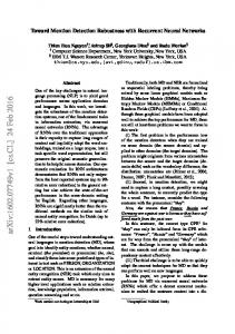
2. SVM with clustering for training SVM are learning systems that use a hypothesis space of linear functions in a high dimensional feature space, trained with a learning algorithm from optimization theory. SVM are based on the idea of a hyper-plane classifier, or linear separability. Suppose we have N training data points {(x1, y1), (x2,y2), (x3, y3), . . . , (xN , yN )}, where xi belong to Rn and yi ∈ {+1,−1}. Consider a hyper-plane defined by (w, b), where w is a weight vector and b is a bias, see fig.1. Details of SVM can be found in [13]. We can classify a new object x with

Note that the training vectors xi occur only in the form of a dot product; there is a Lagrangian multiplier αi for each training point. The Lagrangian multiplier values αi reflect the importance of each data point. When the maximal margin hyper-plane is found, only points that lie closest to the hyper-plane will have αi > 0 and these points are called support vectors. All other points will have αi = 0, see Fig. 1A. This means that only those points that lie closest to the hyper-plane give the representation of the hypothesis/classifier, optimized with minx ||w||2/2 subject to yi(xi•w+b) ≥ 1. 22


Fig. 1: Linear Separation of the SVM

Fig. 2: Separation of the Support Vector points and Non-support Vector points (adapted in part from [12]) These most important data points serve as support vectors. Fig.1A shows two classes and their boundaries, i.e., margins. The support vectors are represented by solid objects, while the empty objects are nonsupport vectors. Notice that the margins are only affected by the support vectors, i.e., if we remove or add empty objects, the margins will not change. Meanwhile any change in the solid objects, either adding or removing objects, could change the margins. Fig.1B shows the effects of adding objects in the margin area. As we can see, adding or removing objects far from the margins, e.g., data point 1 or −2, does not change the margins. However, adding and/or removing objects near the margins, e.g., data point 2 and/or −1, has created new margins. Once this setup, a hierarchy of clustering tree is dynamically constructed.

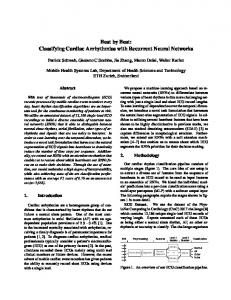
2.1. Clustering tree based on SVM, CT-SVM In this approach, we build a hierarchical clustering tree for each class in the data set (for simplicity and without loss of generality, we assume binary classification) using the DGSOT algorithm. The DGSOT algorithm, top-down clustering, builds the hierarchical tree iteratively in several epochs. After each epoch, new nodes are added to the tree based on a learning process. To avoid the computation overhead of building the tree, we do not build the entire hierarchical trees. Instead, after each epoch we train SVM on the nodes of both trees. We use the support vectors of the classifier as prior knowledge for the succeeding epoch in order to control the tree growth. Specifically, support vectors are allowed to grow, while non-support vectors are stopped. This has the impact of adding nodes in the boundary areas between the two classes, while eliminating distant nodes from the boundaries. Fig. 2 diagrammatically outlines the steps of this approach. First, assuming binary classification, we generate a hierarchical tree for each class in the data set. Initially, we allow the two trees to grow until a certain size of the trees is reached. Basically, we want to start with a reasonable number of nodes. First, if a tree exhibits convergence earlier (i.e., fewer number of nodes), one option is to train SVM with these existing nodes. If the result is unsatisfactory, we will adjust the 23


threshold (profile and radius thresholds). Reducing thresholds may increase number of clusters and nodes. Second, we will train SVM on the nodes of the trees, and compute the support vectors. Third, on the basis of stopping criteria, we either stop the algorithm or continue growing the hierarchical trees. In the case of growing the tree, we use prior knowledge, which consists of the computed support vector nodes, to instruct the DGSOT algorithm to grow support vector nodes, while non-support vector nodes are not grown. By growing a node in the DGSOT algorithm, we mean that we create two children nodes for each support vector node [14].

Fig. 2: Logic Flow diagram of the Approach Flow diagram, Fig. 2, of clustering trees growth of the hierarchical trees. This process has the impact of growing the tree only in the boundary area between the two classes, while stopping the tree from growing in other areas. Hence, we save extensive computations that would have been carried out without any purpose or utility. We can stop at a certain size/level of tree, upon reaching a certain number of nodes/support vectors, and/or when a certain accuracy level is attained. For accuracy level, we can stop the algorithm if the generalization accuracy over a validation set exceeds a specific value (say 98%). For this accuracy estimation, support vectors will be tested with the existing training set based on proximity. In our implementation, we adopt the second strategy (i.e., a certain number of support vectors) so that we can compare our procedure with the Rocchio Bundling algorithm which reduces the data set into a specific size. We do not wait until DGSOT finishes. Instead, after each epoch/iteration of the DGSOT algorithm, we train the SVM on the generated nodes. After each training process we can control the growth of the hierarchical tree from top to bottom because non-support vector nodes will be stopped from growing, and only support vector nodes will be allowed to grow.

Fig. 3: Hierarchy construction using a DGSOT algorithm 24


Fig. 3 shows the growth of one of the hierarchical trees using this approach. The bold nodes represent the support vector nodes. Notice that nodes 1, 2, 3, 5, 6, and 9 are allowed to expand because they are support vector nodes. Meanwhile, we stop nodes 4, 8, 7, and 10 from growing because they are not support vector nodes.

Fig. 4: Selective Growth of the Tree (adapted from [12] and modified) Growing the tree is very important in order to increase the number of points in the data set so as to obtain a more accurate classifier. Fig. 4 shows an illustrative example of growing the tree up to certain size/level and in which we have the training set (+3, +4, +5, +6 + 7, −3, −4, −5, −6, −7). The dashed nodes represent the clusters’ references which are not support vectors. The bold nodes represent the support vector references. Hence, we add the children of the support vector nodes +4 and +7 to the training set. The same applies to the support vector nodes −5 and −7. The new data set now is (+3, +11, +12, +5, +6, +14, +15, −3, −4, −10, −11, −6, −12, −13). Notice that expanded nodes, such as +4 and +7, are excluded because their children nodes are added to the training set. Note that adding new nodes in the boundary area of the old classifier, represented by dashed lines, is corrected and the new classifier, solid lines, is more accurate now than the old one. By doing so, the classifier is adjusted accordingly, creating a more accurate classifier. Beside the selective growth of the tree, the incorporation of the Recurrent Neural Networks (RNN)’s high accuracy in pattern recognition is a critical component of this IDS. Notably, RNN on a comparative basis, out-performed both the feedforward neural networks and the Elman recurrent neural networks.

2.2 Feed-Forward Neural Networks A complete network structure in the simplest level of complexity consists of layers of neurons interconnected in such a way that the output of a neuron in any given position is biased by the inputs it receives, modified by its own weight wk, and which come from many or all of the neurons in the preceding layer. Due to the fact that network connections limit the flow of information within its architecture to a forward direction, without any sort of feedback paths, this kind of network is known as a feed-forward network [15]. Such a network is capable of classifying and identifying patterns of a non-linear network, but its performance across time is limited due to its inability to keep previous states at the beginning of the training. The training is performed following an algorithm for weight update known as Back-propagation [16].

2.3 Elman recurrent neural networks An option in terms of neural network architecture is the Elman network. The main difference between this kind of network and a feed-forward model is the fact that there exist simple 25


feedback paths from a layer to its preceding counterpart, thus enabling the network to store information across time and improve its performance. The Elman network is called a simple recurrent network (SRN) because it is similar to a fully connected network, but the number and complexity of interconnections is lower than in a RNN [15], [17].

2.4 Recurrent neural networks (rnn) An improvement of SRN, fully connected RNN models have feedback connections between all neurons in a layer to the preceding layers, and even feedback connections from a neuron to itself. This increased complexity allows the neuron to store the state of its outputs from the moment the training sequence began up the present. The benefits of this are manifold, as such a network will require less training input vectors to reach a state where it will be suitable for testing patterns it has not been exposed to before, and the fact that it holds a memory of past events will make it easier for the network to classify certain patterns as normal or abnormal with a smaller probability of error. Nevertheless, RNN systems should be trained with a particular kind of algorithm: the Real-Time Recurrent Learning Algorithm (RTRL) [6], [7], [18]. The inputs of an RRN from the first layer are propagated to the layer after it, called the first hidden layer, but also to all other processing elements in all other layers. This means that the outputs of any given neuron in a layer are connected to every other neuron and thus what happens in one affects the changes in the others, specifically modifying the weight parameter. After each output, as well, there is a brief stage of delays purposed to give the network memory of past events in order to use all available information to identify, generalize and predict when faced with new input sequences. The output is passed through a threshold function of sigmoid nature when the process is over and thus the final output yk is obtained.

2.5 Real-time recurrent learning algorithm As its name implies, this training algorithm makes the neural network able to learn and subsequently perform in an online, real-time mode. As opposed to the back-propagation algorithm, RTRL requires significantly greater processing resources: standard back-propagation techniques call for computational resources equal to O(n2), where n is the number of neurons in the entire system, while RTRL calls for O(n4) [7]—a comparatively big difference that has significant impact on larger neural networks, sometimes overriding their inherent benefits. For medium and small networks, nevertheless, this additional processing cost is within acceptable ranges of performance goals [16]. The RTRL algorithm essentially gives a network the capability to use all the information on past outputs since the moment it began training plus the current input to predict the next output sequence.

3. Characteristic features of the proposed system The utility of real-time recurrent learning algorithm avails the neural network’s ability to learn and subsequently perform in an online, real-time mode. This feature cannot be overemphasized, given the dynamic and ever-changing nature of computer network attacks. The noted excellence of neural networks in pattern recognition and parallel computing is an added advantage [5],[6],[7]. Notably, recent studies [19] have shown this feature to be successful even in global efficient systems. A potential deterrent of the incorporation of RTRL algorithm is fourth order crunching time and computing resources. Since most problematic scenarios fall within small to medium levels of complexity, this approach becomes indeed plausible. The effect of this technique is the capability of the network to use all previously acquired information on attacks or network traffic from the initial training along with all presently acquired information to predict the next output sequence. The hyper-plane linear separability of the 26


SVM, coupled with the hierarchically top-down and dynamically growing self-organizing tree (DGSOT) algorithm, not only enable the scalability of the system, but also reduce the false positives and false negatives associated with the precision and recall area in IR and HAC. Furthermore, its top-down functionality enables a selective halting of the growth of the tree when needed by system training.

4. Conclusion The one-size-fits-all format adopted by most existing intrusion detection systems, has not succeeded in eradicating network attacks that are ever-changing in their nature. Furthermore, such IDS is not as economically sustainable for all organizations with unique levels of financial buoyancy, operational complexity, and network traffic. Nevertheless, a scalable IDS, with its several over-reaching advantages that range from adjustable economic costs to easy architectural design and applicability, from fast communication traffic to improved management of IDS, meets the match of the ever-changing nature of network attacks, as well as meeting unique sizes and economic buoyancy of organizations. . It is highly suitable for online real-time applications and its ability to self-adjust to changes in its input environment cannot be overemphasized The limitation of this proposal, however, is its extensive consumption of computing resources for detection systems with large number of neurons.

REFERENCE [1] A. Bivens, C. Palagiri, R. Smith, B. Szymanski, and M. Embrechts, Network-Based Intrusion Detection Using Neural Networks, Intelligent Engineering Systems through Artificial Neural Networks, Proc. Of ANNIE-2002, vol. 12, ASME Press, New York, 2002 pp. 579-584. [2] C. Manikopoulos, C. and S. Papavassiliou, Network Intrusion and Fault Detection: A Statistical Anomaly Approach, IEEE Communications Magazine, October 2002, pp. 76-82. [3] J. P. Planquart, Application of Neural Networks to Intrusion Detection, SANS Institute, July 2001. [4] V. Alarcon-Aquino, J. A. Barria, Anomaly Detection in Communication Networks Using Wavelets, lEEProceedings-Communications, Vol.148, No.6; Dec. 2001; p.355-362. [5] R. P. Lippmann, An Introduction to Computing with Neural Nets, in Neural Networks: Theoretical Foundations and Analysis, Edited by Clifford Lau, IEEE Press, 1992. [6] S. Haykin, Neural Networks^ Prentice Hall, 1998. pp. 274 – 298 [7] J. Willams, D. Zipser, Gradient-Based Learning Algorithm for Recurrent Connectionist Networks. La Jolla, CA Press. California, 1990. pp 1-5 [8] W. Lisheng, X. Zongben, Sufficient and Necessary Conditions for Global Exponential Stability of Discretetime Recurrent Neural Networks, IEEE Transactions on Circuits and Systems I, Vol. 5, Issue 6, June 2006. [9] Voorhees, E.M.: Implementing agglomerative hierarchic clustering algorithms for use in document retrieval, Inform Process Manage. 22(6), 465–476 (1986). [10] Markey MK, Lo JY, Tourassi GD, Floyd CE Jr., Self-organizing map for cluster analysis of a breast cancer database, Artif Intell Med, 2003 Feb;27(2):113-27. [11] H. C. Wang, J. Dopazo, L. G. de la Fraga, Y. P. Zhu, and J. M. Carazo, Self-organizing tree-growing network for the classification of protein sequences, Protein Science, 1998 December; 7(12): 2613–2622. [12] Latifur Khan, Mamoun Awad, Bhavani Thuraisingham, A new intrusion detection system using support vector machines and hierarchical clustering, The VLDB Journal (2007), DOI 10.1007/s00778-006-0002-5. [13] Hisashi Koga, Tetsuo Ishibashi, Toshinori Watanabe, Fast agglomerative hierarchical clustering algorithm using Locality-Sensitive Hashing, Knowledge and Information Systems, Volume 12 , Issue 1, (May 2007) Pages: 25 – 53. [14] Feng Luo, Latifur Khan, Farokh Bastani, I-Ling Yen and Jizhong Zhou,A dynamically growing selforganizing tree (DGSOT) for hierarchical clustering gene expression profiles, Bioinformatics, vol. 20 issue 16, 2004. [15] Vicente Alarcon-Aquino, Carlos A. Oropeza-Clavel, Jorge Rodriguez-Asomoza, Oleg Starostenko, Roberto RosasRomero, Intrusion Detection and Classification of Attacks in High-Level Network Protocols Using Recurrent Neural Networks, CISSE 2008 Proceedings.

27


[16] M. Embrechts, MetaNeura/"" - Hands-on. Rensselaer Polytechnic Institute, Troy NY. 1993. pp. 1- 5, 8 – 13. [17] M. Mak, K. Ku, Y. Lu, On the improvement of the Real-Time Recurrent Learning Algorithm for Recurrent Neural Networks, Department of Electronic Engineering, Hong Kong Polytechnic University, Hong Kong, 1998. pp. 1-4. [18] M. Mak, Application of A Fast Real Time Recurrent Learning Algorithm to Text-to-Phoneme Conversion, Department, of Electronic Engineering, Hong Kong Polytechnic University, Hong Kong, 1995. pp. 1- 5. [19] V. Alarcon-Aquino, J. A. Barria, Multi-resolution FIR Neural-Network-Based Learning Algorithm Applied to Network Traffic Prediction, IEEE Transactions on Systems, Man and Cybernetics Part C: Applications and Review, Vol. 36, Issue No. 2, March 2006. pp. 208-220.

28