Scalable Bayesian Learning of Recurrent Neural Networks for ...

Scalable Bayesian Learning of Recurrent Neural Networks for Language Modeling Zhe Gan, Chunyuan Li, Changyou Chen, Yunchen Pu, Qinliang Su, Lawrence Carin Department of Electrical and Computer Engineering, Duke University {zg27, cl319, cc448, yp42, qs15, lcarin}@duke.edu

arXiv:1611.08034v1 [cs.CL] 23 Nov 2016

Abstract Recurrent neural networks (RNNs) have shown promising performance for language modeling. However, traditional training of RNNs using back-propagation through time often suffers from overfitting. One reason for this is that stochastic optimization (used for large training sets) does not provide good estimates of model uncertainty. This paper leverages recent advances in stochastic gradient Markov Chain Monte Carlo (also appropriate for large training sets) to learn weight uncertainty in RNNs. It yields a principled Bayesian learning algorithm, adding gradient noise during training (enhancing exploration of the model-parameter space) and model averaging when testing. Extensive experiments on various RNN models and across a broad range of applications demonstrate the superiority of the proposed approach over stochastic optimization.

1

Introduction

Language modeling is a fundamental task, used for example to predict the next word or character in a text sequence given the context. Recently, recurrent neural networks (RNNs) have shown promising performance on this task (Mikolov et al., 2010; Sutskever et al., 2011). RNNs with Long Short-Term Memory (LSTM) units (Hochreiter and Schmidhuber, 1997) have emerged as a popular architecture, due to their representational power and effectiveness at capturing long-term dependencies. RNNs are usually trained via back-propagation through time (Werbos, 1990), using stochastic optimization methods such as stochastic gradient de-

scent (SGD) (Robbins and Monro, 1951); stochastic methods of this type are particularly important for training with large data sets. However, this approach often provides a maximum a posteriori (MAP) estimate of model parameters. The MAP solution is a single point estimate, ignoring weight uncertainty (Blundell et al., 2015; HernándezLobato and Adams, 2015). Natural language often exhibits significant variability, and hence such a point estimate may make over-confident predictions on test data. To alleviate this overfitting problem in RNNs, good regularization is known as a key factor to successful applications. In the neural network literature, Bayesian learning has been proposed as a principled method to impose regularization and incorporate model uncertainty (MacKay, 1992; Neal, 1995), by imposing prior distributions on model parameters. Due to the intractability of posterior distributions in neural networks, Hamiltonian Monte Carlo (HMC) (Neal, 1995) has been used to provide sample-based approximations to the true posterior. Despite the elegant theoretical property of asymptotic convergence to the true posterior, HMC and other conventional Markov Chain Monte Carlo methods are not scalable to large training sets. This paper seeks to scale up Bayesian learning of RNNs to meet the challenge of the increasing amount of “big” sequential data in natural language processing, by leveraging recent advances in stochastic gradient Markov Chain Monte Carlo (SG-MCMC) algorithms (Welling and Teh, 2011; Chen et al., 2014; Ding et al., 2014; Li et al., 2016a). Specifically, instead of training a single network, SG-MCMC is employed to train an ensemble of networks, where each network has its parameters drawn from a shared posterior distribution. This is implemented by adding additional gradient noise during training and utilizing model

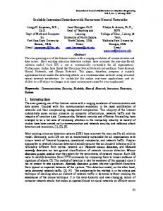
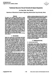
Output Decoding weights Hidden Recurrent weights Input

Encoding weights

Figure 1: Illustration of different weight learning strategies in a single-hidden-layer RNN. Stochastic optimization used for MAP estimation puts fixed values on all weights. Naive dropout is allowed to put weight uncertainty only on encoding and decoding weights, and fixed values on recurrent weights. The proposed SG-MCMC scheme imposes distributions on all weights. averaging when testing. This simple procedure has the following favorable properties for training neural networks: (i) The injected noise encourages model-parameter trajectories when training to better explore the parameter space. This procedure was also empirically found effective in (Neelakantan et al., 2016). (ii) Model averaging when testing alleviates overfitting and hence improves generalization, transferring uncertainty in the learned model parameters to subsequent prediction. (iii) In theory, both asymptotic and non-asymptotic consistency properties of SG-MCMC methods in posterior estimation have been recently established to guarantee convergence (Chen et al., 2015a; Teh et al., 2016). (iv) SG-MCMC is scalable; it shares the same level of computational cost as SGD in training, by only requiring the evaluation of gradients on a small mini-batch. To the authors’ knowledge, RNN training using SG-MCMC has not been investigated previously, and is a contribution of this paper. We also perform extensive experiments on several natural language processing tasks, demonstrating the effectiveness of SG-MCMC for RNNs, including character/word-level language modeling, image captioning and sentence classification.

2

Related Work

Several scalable Bayesian learning methods have been proposed recently for neural networks. These come in two broad categories: stochastic variational inference (Graves, 2011; Blundell et al., 2015; Hernández-Lobato and Adams, 2015) and SG-MCMC methods (Korattikara et al., 2015;

Li et al., 2016a). While prior work focuses on feed-forward neural networks, there has been little if any research reported for RNNs using SGMCMC. Dropout (Hinton et al., 2012; Srivastava et al., 2014) is a commonly used regularization method for training neural networks. Recently, there has been several works on studying how to apply dropout to RNNs (Pachitariu and Sahani, 2013; Bayer et al., 2013; Pham et al., 2014; Zaremba et al., 2014; Bluche et al., 2015; Moon et al., 2015; Semeniuta et al., 2016; Gal and Ghahramani, 2016b). Among them, naive dropout (Zaremba et al., 2014) can impose weight uncertainty only on encoding weights (those that connect input to hidden units) and decoding weights (those that connect hidden units to output), but not the recurrent weights (those that connect consecutive hidden states). It has been concluded that noise added in the recurrent connections leads to model instabilities, hence disrupting the RNN’s ability to model sequences. Dropout has been recently shown to be a variational approximation technique in Bayesian learning (Gal and Ghahramani, 2016a; Kingma et al., 2015). Based on this, (Gal and Ghahramani, 2016b) proposed a new variant of dropout that can be successfully applied to recurrent layers, where the same dropout masks are shared along time for encoding, decoding and recurrent weights, respectively. Alternatively, we focus on SG-MCMC, which can be viewed as the Bayesian interpretation of dropout from the perspective of posterior sampling (Li et al., 2016b); this also allows imposition of model uncertainty on recurrent layers, boosting performance. A comparison of naive dropout and SG-MCMC is illustrated in Fig. 1.

3 3.1

Recurrent Neural Networks RNN as Bayesian Predictive Models

Consider data D = {D1 , · · · , DN }, where Dn , (Xn , Yn ), with input Xn and output Yn . Our goal is to learn model parameters θ to best characterize the relationship from Xn to Yn , with QN corresponding data likelihood p(D|θ) = n=1 p(Dn |θ). In Bayesian statistics, one sets a prior on θ via distribution p(θ). The posterior p(θ|D) ∝ p(θ)p(D|θ) reflects the belief concerning the model parameter distribution after observ˜ (with missing the data. Given a test input X ˜ the uncertainty learned in training ing output Y),

is transferred to prediction, yielding the posterior predictive distribution: Z ˜ X, ˜ θ)p(θ|D)dθ . (1) ˜ ˜ p(Y| p(Y|X, D) = θ

When the input is a sequence, RNNs may be used to parameterize the input-output relationship. Specifically, consider input sequence X = {x1 , . . . , xT }, where xt is the input data vector at time t. There is a corresponding hidden state vector ht at each time t, obtained by recursively applying the transition function ht = H(ht−1 , xt ) (specified in Section 3.2; see Fig. 1). The ouput Y differs depending on the application: a sequence {y1 , . . . , yT } in language modeling or a discrete label in sentence classification. In RNNs the corresponding decoding function is p(y|h), described in Section 3.3. 3.2

RNN Architectures

The transition function H(·) can be implemented with a gated activation function, such as Long Short-Term Memory (LSTM) (Hochreiter and Schmidhuber, 1997) or a Gated Recurrent Unit (GRU) (Cho et al., 2014). Both LSTM and GRU have been proposed to address the issue of learning long-term sequential dependencies. Long Short-Term Memory The LSTM architecture addresses the problem of learning longterm dependencies by introducing a memory cell, that is able to preserve the state over long periods of time. Specifically, each LSTM unit has a cell containing a state ct at time t. This cell can be viewed as a memory unit. Reading or writing the cell is controlled through sigmoid gates: input gate it , forget gate ft , and output gate ot . The hidden units ht are updated as follows: it = σ(Wi xt + Ui ht−1 + bi ) , ft = σ(Wf xt + Uf ht−1 + bf ) , ot = σ(Wo xt + Uo ht−1 + bo ) , c˜t = tanh(Wc xt + Uc ht−1 + bc ) , ct = ft ct−1 + it c˜t , ht = ot tanh(ct ) , where σ(·) denotes the logistic sigmoid function, and represents the element-wise matrix multiplication operator. W{i,f,o,c} are encoding weights, and U{i,f,o,c} are recurrent weights, as shown in Fig. 1. b{i,f,o,c} are bias terms.

Variants Similar to the LSTM unit, the GRU also has gating units that modulate the flow of information inside the hidden unit. It has been shown that a GRU can achieve similar performance to an LSTM in sequence modeling (Chung et al., 2014). We specify the GRU in the Supplementary Material. The LSTM can be extended to the bidirectional LSTM and multilayer LSTM. A bidirectional LSTM consists of two LSTMs that are run in parallel: one on the input sequence and the other on the reverse of the input sequence. At each time step, the hidden state of the bidirectional LSTM is the concatenation of the forward and backward hidden states. In multilayer LSTMs, the hidden state of an LSTM unit in layer ` is used as input to the LSTM unit in layer ` + 1 at the same time step. 3.3

Applications

The proposed Bayesian framework can be applied to any RNN model; we focus on the following basic tasks to demonstrate the ideas. Language Modeling In word-level language modeling, the input to the network is a sequence of words, and the network is trained to predict the next word in the sequence with a softmax classifier. Specifically, for a length-T sequence, denote yt = xt+1 for t = 1, . . . , T − 1. x1 and yT are always set to a special START and END token, respectively. At each time t, there is a decoding function p(yt |ht ) = softmax(Vht ) to compute the distribution over words, where V are the decoding weights (the number of rows of V corresponds to the number of words/characters). We also extend this basic language model to consider other applications: (i) a character-level language model can be specified in a similar manner by replacing words with characters (Karpathy et al., 2016). (ii) Image captioning can be considered as a conditional language modeling problem, in which we learn a generative language model of the caption conditioned on an image (Vinyals et al., 2015). Sentence Classification Sentence classification aims to assign a semantic category label y to a whole sentence X. This is usually implemented through applying the decoding function once at the end of sequence: p(y|hT ) = softmax(VhT ), where the final hidden state of a RNN hT is often considered as the summary of the sentence (here

the number of rows of V corresponds to the number of classes).

4 4.1

Scalable Learning with SG-MCMC The Pitfall of Stochastic Optimization

Typically there is no closed-form solution for (1), and traditional MCMC methods scale poorly for large N . To ease the computational burden, stochastic optimization is often employed to find the MAP solution. This is equivalent to minimizing an objective of regularized loss function U (θ) that corresponds to a (non-convex) model of interest: θMAP = arg min U (θ), U (θ) = − log p(θ|D). The expectation in (1) is approximated as: ˜ X, ˜ D) = p(Y| ˜ X, ˜ θMAP ) . p(Y|

(2)

Though simple and effective, this procedure largely loses the benefit of the Bayesian approach, because the uncertainty on weights is ignored. To more accurately approximate (1), we employ SGMCMC. 4.2

Large-scale Bayesian Learning

In a Bayesian model, the above regularized loss function corresponds to the potential energy defined as the negative log-posterior: U (θ) , − log p(θ) −

N X

log p(Dn |θ).

(3)

n=1

PN

In optimization, E = − n=1 log p(Dn |θ) is typically referred to as the loss function, and R ∝ − log p(θ) as a regularizer. For large N , stochastic approximations are often employed: M X ˜t (θ), − log p(θ) − N U log p(Dim |θ), (4) M m=1

where Sm = {i1 , · · · , iM } is a random subset of the set {1, 2, · · · , N }, with M N . The gradi˜t (θ), ent on this mini-batch is denoted as f˜t = ∇U which is an unbiased estimate of the true gradient. The evaluation of (4) is cheap even when N is large, allowing one to efficiently collect a sufficient number of samples in large-scale Bayesian learning, {θs }Ss=1 , where S is the number of samples (this will be specified later). These samples are used to construct a sample-based estimation to the expectation in (1):

Table 1: SG-MCMC algorithms and their optimization counterparts. Algorithms in the same row share similar characteristics. Algorithms Basic Precondition Momentum Thermostat

SG-MCMC SGLD pSGLD SGHMC SGNHT

Optimization SGD RMSprop/Adagrad momentum SGD Santa

S 1X ˜ ˜ ˜ ˜ p(Y|X, θs ) . p(Y|X, D) ≈ S

(5)

s=1

The finite-time estimation errors of SG-MCMC methods are bounded (Chen et al., 2015a), which guarantees (5) is an unbiased estimate of (1) asymptotically under appropriate decreasing stepsizes. 4.3

SG-MCMC Algorithms

SG-MCMC and stochastic optimization are two parallel lines of work, designed for different purposes; their relationship has recently been revealed in the context of deep learning. The most basic SG-MCMC algorithm has been applied to Langevin dynamics, and is termed SGLD (Welling and Teh, 2011). To help convergence, a momentum term has been introduced in SGHMC (Chen et al., 2014), a “thermostat” has been devised in SGNHT (Ding et al., 2014; Gan et al., 2015) and preconditioners have been employed in pSGLD (Li et al., 2016a). These SG-MCMC algorithms often share similar characteristics with their counterpart approaches from the optimization literature such as the momentum SGD, Santa (Chen et al., 2016) and RMSprop/Adagrad (Tieleman and Hinton, 2012; Duchi et al., 2011). The interrelationships between SG-MCMC and optimizationbased approaches are summarized in Table 1. SGLD Stochastic Gradient Langevin Dynamics (SGLD) (Welling and Teh, 2011) draws posterior samples, with updates p θt = θt−1 − ηt f˜t−1 + 2ηt ξt , (6) where ηt is the learning rate, and ξt ∼ N (0, Ip ) is a standard Gaussian random vector. SGLD is the SG-MCMC analog to SGD, whose parameter updates are given by: θt = θt−1 − ηt f˜t−1 .

(7)

Algorithm 1: pSGLD Input: Default hyperparameter settings: ηt = 1×10−3 , λ = 10−8 , β1 = 0.99. Initialize: v0 ← 0, θ1 ∼ N (0, I) ; for t = 1, 2, . . . , T do

with the nonlinear function q(·) and consecutive layers h1 and h2 , dropout and dropConnect are denoted as: Dropout: DropConnect:

% Estimate gradient from minibatch St

˜t (θ); f˜t = ∇U % Preconditioning

vt ← β1 vt−1 + (1 − β1 )f˜t f˜t ; 1 2 G−1 ← diag 1 λ1 + v ; t t

SGD is guaranteed to converge to a local minimum under mild conditions (Bottou, 2010). The additional Gaussian term in SGLD helps the learning trajectory to explore the parameter space to approximate posterior samples, instead of obtaining a local minimum. pSGLD Preconditioned SGLD (pSGLD) (Li et al., 2016a) was proposed recently to improve the mixing of SGLD. It utilizes magnitudes of recent gradients to construct a diagonal preconditioner to approximate the Fisher information matrix, and thus adjusts to the local geometry of parameter space by equalizing the gradients so that a constant stepsize is adequate for all dimensions. This is important for RNNs, whose parameter space often exhibits pathological curvature and saddle points (Pascanu et al., 2013), resulting in slow mixing. There are multiple choices of preconditioners; similar ideas in optimization include Adagrad (Duchi et al., 2011), Adam (Kingma and Ba, 2015) and RMSprop (Tieleman and Hinton, 2012). An efficient version of pSGLD, adopting RMSprop as the preconditioner G, is summarized in Algorithm 1, where denotes element-wise matrix division. When the preconditioner is fixed as the identity matrix, the method reduces to SGLD. 4.4

Understanding SG-MCMC

To further understand SG-MCMC, we show its close connection to dropout/dropConnect (Srivastava et al., 2014; Wan et al., 2013). These methods improve the generalization ability of deep models, by randomly adding binary/Gaussian noise to the local units or global weights. For neural networks

h2 = q((ξ0 θ)h1 ),

where the injected noise ξ0 can be binary-valued with dropping rate p or its equivalent Gaussian form (Wang and Manning, 2013): Binary noise:

% Parameter update

ξt ∼ N (0, ηt G−1 t ); ηt −1 ˜ θt+1 ← θt + 2 Gt ft + ξt ; end

h2 = ξ0 q(θh1 ),

Gaussian noise:

ξ0 ∼ Ber(p), ξ0 ∼ N (1,

p ). 1−p

Note that ξ0 is defined as a vector for dropout, and a matrix for dropConnect. By combining dropConnect and Gaussian noise from the above, we have the update rule (Li et al., 2016b): η η θt+1 = ξ0 θt − f˜t = θt − f˜t + ξ00 , (8) 2 2 p where ξ00 ∼ N 0, (1−p) diag(θt2 ) ; (8) shows that dropout/ dropConnect and SGLD in (6) share the same form of update rule, with the distinction being that the level of injected noise is different. In practice, the noise injected by SGLD may not be enough. A better way that we find to improve the performance is to jointly apply SGLD and dropout. This method can be interpreted as using SGLD to sample the posterior distribution of a mixture of RNNs, with mixture probability controlled by the dropout rate.

5

Experiments

We present results on several tasks, including character/ word-level language modeling, image captioning, and sentence classification. The hyperparameter setting, the initialization of model parameters and model specifications on each dataset are all provided in the Supplementary Material. We do not perform any dataset-specific tuning other than early stopping on validation sets. When dropout is utilized, the dropout rate is empirically set to 0.5. All experiments are implemented in Theano (Theano Development Team, 2016), using a NVIDIA GeForce GTX TITAN X GPU with 12GB memory. 5.1

Language Modeling

We first test character-level and word-level language modeling. The setup for each task is as follows.

• Following (Karpathy et al., 2016), we test character-level language modeling on the War and Peace (WP) novel. The training/validation/test sets contain 260/32/33 batches, in which there are 100 characters. The vocabulary size is 87, and we consider a 2-hidden-layer RNN of dimension 128.

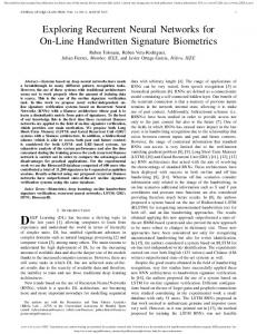
We study the effects of different types of architecture (LSTM/GRU/Vanilla RNN) on the WP dataset, and effects of different learning algorithms on the PTB dataset. The comparison of test cross-entropy loss on WP is shown in Table 2. We observe that pSGLD consistently outperforms RMSprop. Table 3 summarizes the test set performance on PTB1 . It is clear that our sampling-based method consistently outperforms the optimization counterpart, where the performance gain mainly comes from adding gradient noise and model averaging. When compared with dropout, SGLD performs better on the small LSTM model, but slightly worse on the medium and large LSTM model. This may imply that dropout is suitable to regularizing large networks, while SGLD exhibits better regularization ability on small networks, partially due to the fact that dropout may inject a higher level of noise during training than SGLD. In order to inject a higher level of noise into SGLD, we empirically apply SGLD and dropout jointly, and found that this provided the best performace on the medium and large LSTM model. We study three strategies to do model averaging, i.e., forward collection, backward collection and thinned collection. Given samples (θ1 , · · · , θK ) and the number of samples S used for averaging, forward collection refers to using (θ1 , · · · , θS ) for the evaluation of a test function, backward collection refers to using (θK−S+1 , · · · , θK ), while 1

The results reported here do not match (Zaremba et al., 2014) due to the differences of experimental setup. However, we provide a fair comparison to all methods.

Table 3: Test perplexity on Penn Treebank. Methods Small Medium Large SGD 123.85 126.31 130.25 SGD+Dropout 136.39 100.12 97.65 SGLD 117.36 109.14 105.86 SGLD+Dropout 139.54 99.58 94.03 180 170 160 150 140 130 120 110

Perplexity

Perplexity

• The Penn Treebank (PTB) corpus (Marcus et al., 1993) is used for word-level language modeling. The dataset adopts the standard split (929K training words, 73K validation words, and 82K test words) and has a vocabulary of size 10K. We train LSTMs of three sizes; these are denoted the small/medium/large LSTM. All LSTMs have two layers and are unrolled for 20 steps. The small, medium and large LSTM has 200, 650 and 1500 units per layer, respectively.

Table 2: Test cross-entropy loss on WP dataset. Methods LSTM GRU RNN RMSprop 1.3607 1.2759 1.4239 pSGLD 1.3375 1.2561 1.4093

10

20 30 40 Individual Sample

(a) Single sample

50

60

180 170 160 150 140 130 120 110

forward collection backward collection thinned collection

0

10

20

30

40

50

60

Number of Samples for Model Averaging

(b) Different collections

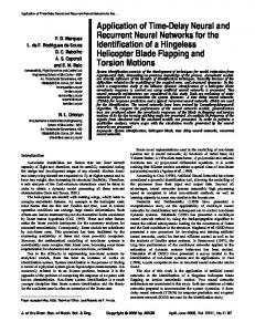
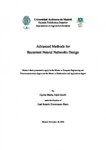
Figure 2: Effects of collected samples. thinned collection chooses samples from θ1 to θK with interval K/S. Fig. 2 plots the effects of these strategies, where Fig. 2(a) plots the perplexity of every single sample, Fig. 2(b) plots the perplexities using the three schemes. It can be seen that only after 20 samples is a converged perplexity achieved in the thinned collection, while it requires 30 samples for forward collection or 60 samples for backward collection. This is unsurprising, because thinned collection provides a better way to select samples. Nevertheless, averaging of samples provides significantly lower perplexity than using single samples. Note that the overfitting problem in Fig. 2(a) is also alleviated by model averaging. To better illustrate the benefit of model averaging, we visualize in Fig. 3 the probabilities of each word in a randomly chosen test sentence. The first 3 rows are the results predicted by 3 distinctive model samples, respectively; the bottom row is the result after averaging. Their corresponding perplexities for the test sentence are also shown on the right of each row. The 3 individual samples provide reasonable probabilities. For example, the consecutive words “New York”, “stock exchange” and “did not” are assigned with a higher probability. After averaging, we can see a much lower perplexity, as the samples can complement each other. For example, though the second sample can

Table 4: Performance on Flickr8k & Flickr30k datasets in terms of BLEU-1,2,3,4, METEOR, CIDEr, ROUGE-L and perplexity. Methods Results on Flickr8k RMSprop RMSprop + Dropout pSGLD pSGLD + Dropout Results on Flickr30k RMSprop RMSprop + Dropout pSGLD pSGLD + Dropout

B-1

B-2

B-3

B-4

METEOR

CIDEr

ROUGE-L

Perp.

0.640 0.647 0.669 0.656

0.427 0.444 0.463 0.450

0.288 0.305 0.321 0.309

0.197 0.209 0.224 0.211

0.205 0.208 0.214 0.209

0.476 0.514 0.535 0.512

0.500 0.510 0.522 0.512

16.64 15.72 14.29 14.26

0.644 0.656 0.657 0.666

0.422 0.435 0.438 0.448

0.279 0.295 0.300 0.308

0.184 0.200 0.206 0.209

0.180 0.185 0.192 0.189

0.372 0.396 0.421 0.419

0.476 0.481 0.490 0.487

17.80 18.05 15.61 17.05

the new york stock exchange did not fall apart 25.55

1 0.8


0.6


0.4


0.2 0

Figure 3: Predictive probabilities obtained by 3 samples and their average. Colors indicate normalized probability of each word. Best viewed in color. yield the lowest single-model perplexity, its prediction on word “York” is still benefited from the other two via averaging. 5.2

a"tan"dog"is"playing"in"the"grass a"tan"dog"is"playing"with"a"red"ball"in"the"grass a"tan"dog"with"a"red"collar"is"running"in"the"grass a"yellow"dog"runs"through"the"grass a"yellow"dog"is"running"through"the"grass a"brown"dog"is"running"through"the"grass a"group"of"people"stand"in"front"of"a"building a"group"of"people"stand"in"front"of"a"white"building a"group"of"people"stand"in"front"of"a"large"building a"man"and"a"woman"walking"on"a"sidewalk a"man"and"a"woman"stand"on"a"balcony a"man"and"a"woman"standing"on"the"ground

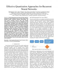
Figure 4: Image captioning with different samples. Left are the given images, right are the corresponding captions. The captions in each box are from the same model sample.

Image Caption Generation

We next consider the problem of image caption generation, which is a conditional RNN model, where image features are extracted by residual network (He et al., 2016), and then fed into the RNN to generate the caption. We present results on two benchmark datasets, Flickr8k (Hodosh et al., 2013) and Flickr30k (Young et al., 2014). These datasets contain 8,000 and 31,000 images, respectively. Each image is annotated with 5 sentences. A single-layer LSTM is employed with the number of hidden units set to 512. The widely used BLEU (Papineni et al., 2002), METEOR (Banerjee and Lavie, 2005), ROUGEL (Lin, 2004), and CIDEr-D (Vedantam et al., 2015) metrics are used to evaluate the performance. All the metrics are computed by using the code released by the COCO evaluation server (Chen et al., 2015b). Table 4 presents results for pSGLD/RMSprop with or without dropout. Consistent with the results in the basic language modeling, pSGLD

yields improved performance compared to RMSprop. For example, pSGLD provides 2.77 BLEU-4 score improvement over RMSprop on the Flickr8k dataset. By comparing pSGLD with RMSprop with dropout, we conclude that pSGLD exhibits better regularization ability than dropout on these two datasets. Apart from modeling weight uncertainty, different samples from our algorithm may capture different aspects of the input image. An example with two images is shown in Fig. 4, where 2 randomly chosen model samples are considered for each image. For each model sample, the top 3 generated captions are presented. We use the beam search approach (Vinyals et al., 2015) to generate captions, with a beam of size 5. In Fig. 4, the two samples for the first image mainly differ in the color and activity of the dog, e.g., “tan” or “yellow”, “playing” or “running”, whereas for the second image, the two samples reflect different understanding of the image content.

Table 5: Sentence classification errors on five benchmark datasets. Methods RMSprop RMSprop + Dropout RMSprop + Gal’s Dropout pSGLD pSGLD + Dropout Train

0.15 0.10

0.16

MPQA 10.60±1.28 10.66±0.74 10.59±1.12 10.54±0.99 10.22±0.89

What does cc in engines mean?

0.20 0.18

SUBJ 8.13±1.19 7.24±0.86 7.52±1.17 7.43±1.21 6.61±1.06 Testing5Question

0.20

0.22

0.14

0.05

CR 22.70±2.20 20.70±2.22 20.21±2.34 21.18±1.90 19.74±2.03

Test

0.24

Error

Error

0.20

Validation

0.26

RMSprop RMSprop + Dropout pSGLD pSGLD + Dropout

Error

0.25

MR 21.26±1.45 20.33±0.67 19.66±0.60 20.36±1.09 19.48±0.95

What does a defibrillator do?

0.15

TREC 8.58±0.79 7.82±0.66 8.32±0.52 7.88±0.72 7.32±0.66

True5Type

Predicted5 Type

Description

Abbreviation

Description

Entity

0.10

0.12

0.00

5

10

#Epoch

15

0.10

5

10

#Epoch

15

5

10

#Epoch

15

Figure 5: Learning curves on TREC dataset. 5.3

Sentence Classification

We study the task of sentence classification on 5 datasets as in (Kiros et al., 2015): TREC (Li and Roth, 2002), MR (Pang and Lee, 2005), SUBJ (Pang and Lee, 2004), CR (Hu and Liu, 2004) and MPQA (Wiebe et al., 2005). A detailed description of the datasets is provided in the Supplementary Material. A single-layer bidirectional LSTM is employed with the number of hidden units set to 400. Table 5 shows the testing classification errors. 10-fold cross-validation is used for evaluation on the first 4 datasets, while TREC has a pre-defined training/test split, and we run each algorithm 10 times on TREC. In addition to (naive) dropout, we further compare pSGLD with the Gal’s dropout, recently proposed in (Gal and Ghahramani, 2016b), which is shown to be applicable to recurrent layers. The combination of pSGLD and dropout consistently provides the lowest errors. In the following, we focus on the analysis of TREC. Each sentence of TREC is a question, and the goal is to decide which topic type the question is most related to: location, human, numeric, abbreviation, entity or description. Fig. 5 plots the learning curves of different algorithms on the training, validation and testing sets of the TREC dataset. pSGLD and dropout have similar behavior: they explore the parameter space during learning, and thus coverge slower than RSMprop on the training dataset. However, the learned uncertainty

Figure 6: Visualization. Top two rows show selected ambiguous sentences, which correspond to the points with black circles in tSNE visualization of the testing dataset. alleviates overfitting and results in lower errors on the validation and testing datasets. To further study the Bayesian nature of the proposed approach, in Fig. 6 we choose two testing sentences with high uncertainty (i.e., standard derivation in prediction) from the TREC dataset. Interestingly, after embedding to 2d-space with tSNE (Van der Maaten and Hinton, 2008), the two sentences correspond to points lying on the boundary of different classes. We use 20 model samples to estimate the prediction mean and standard derivation on the true type and predicted type. The classifier yields higher probability on the wrong types, associated with higher standard derivations. One can leverage the uncertainty information to make decisions: either manually make a human judgement when uncertainty is high, or automatically choose the one with lower standard derivations when both types exhibits similar prediction means. A more rigorous usage of the uncertainty information is left as future work.

6

Conclusion

We propose a scalable Bayesian learning framework using SG-MCMC, to model weight uncertainty in recurrent neural networks. The learn-

ing framework is tested on several tasks, including language models, image caption generation and sentence classification. Our algorithm outperforms conventional stochastic optimization algorithms, indicating the importance of learning weight uncertainty in recurrent neural networks. Our algorithm requires little additional computational overhead in training, and multiple times of forward-passing for model averaging in testing. Future works include improving the testing efficiency for the large-scale RNNs, via learning a single neural network that approximates the model averaging result (Korattikara et al., 2015).

Acknowledgments This research was supported in part by ARO, DARPA, DOE, NGA, ONR and NSF.

References [Banerjee and Lavie2005] Satanjeev Banerjee and Alon Lavie. 2005. Meteor: An automatic metric for mt evaluation with improved correlation with human judgments. In ACL workshop. [Bayer et al.2013] J. Bayer, C. Osendorfer, D. Korhammer, N. Chen, S. Urban, and P. van der Smagt. 2013. On fast dropout and its applicability to recurrent networks. arXiv:1311.0701. [Bluche et al.2015] T. Bluche, C. Kermorvant, and J. Louradour. 2015. Where to apply dropout in recurrent neural networks for handwriting recognition? In ICDAR. [Blundell et al.2015] C. Blundell, J. Cornebise, K. Kavukcuoglu, and D. Wierstra. 2015. Weight uncertainty in neural networks. In ICML. [Bottou2010] L Bottou. 2010. Large-scale machine learning with stochastic gradient descent. In COMPSTAT. [Chen et al.2014] T. Chen, E. B. Fox, and C. Guestrin. 2014. Stochastic gradient Hamiltonian Monte Carlo. In ICML. [Chen et al.2015a] C. Chen, N. Ding, and L. Carin. 2015a. On the convergence of stochastic gradient MCMC algorithms with high-order integrators. In NIPS.

stochastic gradient MCMC and stochastic optimization. In AISTATS. [Cho et al.2014] K. Cho, B. Van Merriënboer, C. Gulcehre, D. Bahdanau, F. Bougares, H. Schwenk, and Y. Bengio. 2014. Learning phrase representations using RNN encoder-decoder for statistical machine translation. In EMNLP. [Chung et al.2014] J. Chung, C. Gulcehre, K. Cho, and Y. Bengio. 2014. Empirical evaluation of gated recurrent neural networks on sequence modeling. arXiv:1412.3555. [Ding et al.2014] N. Ding, Y. Fang, R. Babbush, C. Chen, R. D. Skeel, and H. Neven. 2014. Bayesian sampling using stochastic gradient thermostats. In NIPS. [Duchi et al.2011] J. Duchi, E. Hazan, and Y. Singer. 2011. Adaptive subgradient methods for online learning and stochastic optimization. JMLR. [Gal and Ghahramani2016a] Y. Gal and Z. Ghahramani. 2016a. Dropout as a Bayesian approximation: Representing model uncertainty in deep learning. In ICML. [Gal and Ghahramani2016b] Y. Gal and Z. Ghahramani. 2016b. A theoretically grounded application of dropout in recurrent neural networks. In NIPS. [Gan et al.2015] Z. Gan, C. Chen, R. Henao, D. Carlson, and L. Carin. 2015. Scalable deep poisson factor analysis for topic modeling. In ICML. [Graves2011] A. Graves. 2011. Practical variational inference for neural networks. In NIPS. [He et al.2016] Kaiming He, Xiangyu Zhang, Shaoqing Ren, and Jian Sun. 2016. Deep residual learning for image recognition. In CVPR. [Hernández-Lobato and Adams2015] J. M. HernándezLobato and R. P. Adams. 2015. Probabilistic backpropagation for scalable learning of Bayesian neural networks. In ICML. [Hinton et al.2012] G. Hinton, N. Srivastava, A. Krizhevsky, I. Sutskever, and R Salakhutdinov. 2012. Improving neural networks by preventing co-adaptation of feature detectors. arXiv:1207.0580. [Hochreiter and Schmidhuber1997] S. Hochreiter and J. Schmidhuber. 1997. Long short-term memory. In Neural computation.

[Chen et al.2015b] Xinlei Chen, Hao Fang, Tsung-Yi Lin, Ramakrishna Vedantam, Saurabh Gupta, Piotr Dollár, and C Lawrence Zitnick. 2015b. Microsoft coco captions: Data collection and evaluation server. arXiv:1504.00325.

[Hodosh et al.2013] M. Hodosh, P. Young, and J. Hockenmaier. 2013. Framing image description as a ranking task: Data, models and evaluation metrics. JAIR.

[Chen et al.2016] C. Chen, D. Carlson, Z. Gan, C. Li, and L. Carin. 2016. Bridging the gap between

[Hu and Liu2004] M. Hu and B. Liu. 2004. Mining and summarizing customer reviews. SIGKDD.

[Karpathy et al.2016] A. Karpathy, J. Johnson, and L. Fei-Fei. 2016. Visualizing and understanding recurrent networks. In ICLR Workshop. [Kingma and Ba2015] D. Kingma and J. Ba. 2015. Adam: A method for stochastic optimization. In ICLR. [Kingma et al.2015] D. Kingma, T. Salimans, and M. Welling. 2015. Variational dropout and the local reparameterization trick. In NIPS. [Kiros et al.2015] Ryan Kiros, Yukun Zhu, Ruslan Salakhutdinov, Richard Zemel, Raquel Urtasun, Antonio Torralba, and Sanja Fidler. 2015. Skipthought vectors. In NIPS. [Korattikara et al.2015] A. Korattikara, V. Rathod, K. Murphy, and M. Welling. 2015. Bayesian dark knowledge. In NIPS. [Le et al.2015] Q. V. Le, N. Jaitly, and G. E. Hinton. 2015. A simple way to initialize recurrent networks of rectified linear units. arXiv:1504.00941.

[Neelakantan et al.2016] A. Neelakantan, L. Vilnis, Q. Le, I. Sutskever, L. Kaiser, K. Kurach, and J. Martens. 2016. Adding gradient noise improves learning for very deep networks. In ICLR workshop. [Pachitariu and Sahani2013] M. Pachitariu and M. Sahani. 2013. Regularization and nonlinearities for neural language models: when are they needed? arXiv:1301.5650. [Pang and Lee2004] B. Pang and L. Lee. 2004. A sentimental education: Sentiment analysis using subjectivity summarization based on minimum cuts. ACL. [Pang and Lee2005] B. Pang and L. Lee. 2005. Seeing stars: Exploiting class relationships for sentiment categorization with respect to rating scales. ACL. [Papineni et al.2002] Kishore Papineni, Salim Roukos, Todd Ward, and Wei-Jing Zhu. 2002. Bleu: a method for automatic evaluation of machine translation. In ACL.

[Li and Roth2002] X. Li and D. Roth. 2002. Learning question classifiers. ACL.

[Pascanu et al.2013] R. Pascanu, T. Mikolov, and Y. Bengio. 2013. On the difficulty of training recurrent neural networks. In ICML.

[Li et al.2016a] C. Li, C. Chen, D. Carlson, and L. Carin. 2016a. Preconditioned stochastic gradient Langevin dynamics for deep neural networks. In AAAI.

[Pham et al.2014] V. Pham, T. Bluche, C. Kermorvant, and J. Louradour. 2014. Dropout improves recurrent neural networks for handwriting recognition. In ICFHR.

[Li et al.2016b] C. Li, A. Stevens, C. Chen, Y. Pu, Z. Gan, and L. Carin. 2016b. Learning weight uncertainty with stochastic gradient MCMC for shape classification. In CVPR.

[Robbins and Monro1951] H. Robbins and S. Monro. 1951. A stochastic approximation method. In The annals of mathematical statistics.

[Lin2004] Chin-Yew Lin. 2004. Rouge: A package for automatic evaluation of summaries. In ACL workshop.

[Saxe et al.2014] A. M. Saxe, J. L. McClelland, and S. Ganguli. 2014. Exact solutions to the nonlinear dynamics of learning in deep linear neural networks. In ICLR.

[MacKay1992] D. J. C. MacKay. 1992. A practical Bayesian framework for backpropagation networks. In Neural computation.

[Semeniuta et al.2016] S. Semeniuta, A. Severyn, and E. Barth. 2016. Recurrent dropout without memory loss. arXiv:1603.05118.

[Marcus et al.1993] M. P. Marcus, M. A. Marcinkiewicz, and B. Santorini. 1993. Building a large annotated corpus of english: The penn treebank. Computational linguistics.

[Srivastava et al.2014] N. Srivastava, G. Hinton, A. Krizhevsky, I. Sutskever, and R. Salakhutdinov. 2014. Dropout: A simple way to prevent neural networks from overfitting. JMLR.

[Mikolov et al.2010] T. Mikolov, M. Karafiát, L. Burget, J. Cernock`y, and S. Khudanpur. 2010. Recurrent neural network based language model. In INTERSPEECH.

[Sutskever et al.2011] I. Sutskever, J. Martens, and G. E. Hinton. 2011. Generating text with recurrent neural networks. In ICML.

[Mikolov et al.2013] T. Mikolov, I. Sutskever, K. Chen, G. S. Corrado, and J. Dean. 2013. Distributed representations of words and phrases and their compositionality. In NIPS. [Moon et al.2015] T. Moon, H. Choi, H. Lee, and I. Song. 2015. Rnndrop: A novel dropout for rnns in asr. ASRU. [Neal1995] R. M. Neal. 1995. Bayesian learning for neural networks. PhD thesis, University of Toronto.

[Sutskever et al.2014] I. Sutskever, O. Vinyals, and Q. V. Le. 2014. Sequence to sequence learning with neural networks. In NIPS. [Teh et al.2016] Y. W. Teh, A. H. Thiéry, and S. J. Vollmer. 2016. Consistency and fluctuations for stochastic gradient Langevin dynamics. JMLR. [Theano Development Team2016] Theano Development Team. 2016. Theano: A Python framework for fast computation of mathematical expressions. arXiv:1605.02688.

[Tieleman and Hinton2012] T. Tieleman and G. Hinton. 2012. Lecture 6.5-rmsprop: Divide the gradient by a running average of its recent magnitude. Coursera: Neural Networks for Machine Learning.

where σ(·) denotes the logistic sigmoid function, and represents the element-wise multiply operator. W{r,z,h} are encoding weights, and U{r,z,h} are recurrent weights. b{r,z,h} are bias terms.

[Van der Maaten and Hinton2008] L. Van der Maaten and G. E. Hinton. 2008. Visualizing data using tSNE. JMLR.

B

[Vedantam et al.2015] Ramakrishna Vedantam, C Lawrence Zitnick, and Devi Parikh. 2015. Cider: Consensus-based image description evaluation. In CVPR. [Vinyals et al.2015] O. Vinyals, A. Toshev, S. Bengio, and D. Erhan. 2015. Show and tell: A neural image caption generator. In CVPR. [Wan et al.2013] L. Wan, M. Zeiler, S. Zhang, Y. LeCun, and R. Fergus. 2013. Regularization of neural networks using DropConnect. In ICML. [Wang and Manning2013] S. Wang and C. Manning. 2013. Fast Dropout training. In ICML. [Welling and Teh2011] M. Welling and Y. W. Teh. 2011. Bayesian learning via stochastic gradient Langevin dynamics. In ICML. [Werbos1990] P. Werbos. 1990. Backpropagation through time: what it does and how to do it. In Proceedings of the IEEE. [Wiebe et al.2005] J. Wiebe, T. Wilson, and C. Cardie. 2005. Annotating expressions of opinions and emotions in language. Language resources and evaluation. [Young et al.2014] P. Young, A. Lai, M. Hodosh, and J. Hockenmaier. 2014. From image descriptions to visual denotations: New similarity metrics for semantic inference over event descriptions. TACL. [Zaremba et al.2014] W. Zaremba, I. Sutskever, and O. Vinyals. 2014. Recurrent neural network regularization. arXiv:1409.2329.

B.1

For an input sequence X = {x1 , . . . , xT }, where xt is the input data vector at time t, we define an output sequence Y = {y1 , . . . , yT } with yt = xt+1 for t = 1, . . . , T − 1. x1 and yT are always set to a special START and END token, respectively. The probability p(Y|X) is defined as p(Y|X) =

T Y

p(yt |x≤t ) =

t=1

(9)

zt = σ(Wz xt + Uz ht−1 + bz ) , (10) ˜ t = tanh(Wh xt + Uh (rt ht−1 ) + bh ) , h (11) ˜t , ht = (1 − zt ) ht−1 + zt h (12)

p(yt |ht ) . (13)

t=1

B.2

Image Captioning

Image caption generation is considered as a conditional language modeling problem, where image features are first extracted by residual network (He et al., 2016) as a preprocessing step, and then fed into the RNN to generate the caption. Denote z as the image feature vector, using the same notation as in standard language modeling, the probablity p(Y|X, z) is defined as T Y

p(yt |x≤t , z) =

t=1

Similar to the LSTM unit, the GRU (Cho et al., 2014) has gating units that modulate the flow of information inside the unit, however, without using a separate memory cell. Specifically, the GRU has two gates: the reset gate rt and the update gate zt . The hidden units ht are updated as follows:

T Y

At each time t, there is a decoding function p(yt |ht ) = softmax(Vht ) to compute the distribution over words, where V are the decoding weights. The hidden states are recursively updated by ht = H(ht−1 , xt ), where H is a nonlinear function such as the LSTM or GRU defined above.

Gated Recurrent Units

rt = σ(Wr xt + Ur ht−1 + br ) ,

Standard Language Modeling

p(Y|X, z) =

Supplementary Material A

Model Details

T Y

p(yt |ht ) .

t=1

The only difference with a standard language model is that at the first time step, we use the image feature vector z to update h1 = H(h0 , x1 , z). h0 is set to a zero vector. The hidden states at other time steps are recursively updated by ht = H(ht−1 , xt ), as in standard language modeling. Note that the image feature vector z is only used to generate the first word, which works better in practice than when being used at each time step of the RNN (Vinyals et al., 2015).

C

SGLD Algorithm

We list the SGLD algorithm below for clarity.

Table 6: Hyper-parameter settings of pSGLD for different datasets. For the PTB dataset, the setting is used for SGLD. Datasets Minibatch Size Step Size # Total Epoch Burn-in (#Epoch) Thinning Interval (#Epoch) # Samples Collected

WP 100 2×10−3 20 4 1/2 32

PTB 32 1 40 4 1/2 72

Flickr8k 64 10−3 20 3 1 17

Algorithm 2: SGLD Input: Learning rate schedule {ηt }Tt=1 . Initialize: θ1 ∼ N (0, I) ; for t = 1, 2, . . . , T do % Estimate gradient from minibatch Sm

˜t (θ); f˜t = ∇U % Parameter update

ξt ∼ N (0, ηt I); θt+1 ← θt + η2t f˜t + ξt ; end

D

Experimental Setup

For RNN training, orthogonal initialization is employed on all recurrent matrices (Saxe et al., 2014). Non-recurrent weights are initialized from a uniform distribution in [−0.01, 0.01]. All the bias terms are initialized to zero. It is observed that setting a high initial forget gate bias for LSTMs can give slightly better results (Le et al., 2015). Hence, the initial forget gate bias is set to 3 throughout the experiments. Word vectors are initialized with the publicly available word2vec vectors (Mikolov et al., 2013). These vectors have dimensionality 300 and were trained using a continuous bag-of-words architecture . Words not present in the set of pre-trained words are initialized at random. Gradients are clipped if the norm of the parameter vector exceeds 5 (Sutskever et al., 2014). The hyperparameters for the algorithm include stepsize, minibatch size, thinning interval, number of burn-in epochs and variance of the Gaussian priors. We explain some hyperparameters that are unique in pSGLD and list the specific values used in our experiments in Table 6. RMSprop employs the same hyperparameter setting as pSGLD. Throughout the experiments, the dropout rate is set to 0.5. The learning rate for SGD and SGLD (used in the word-level language modeling) is set to 1. For

Flickr30k 64 10−3 20 3 1/2 34

MR 50 10−3 20 1 1 19

CR 50 10−3 20 1 1 19

SUBJ 50 10−3 20 1 1 19

MPQA 50 10−3 20 1 1 19

TREC 50 10−3 20 1 1 19

the small LSTM model, we halved the learning rate every epoch after the 4th. For the medium LSTM model, we decrease the learning rate by a factor of 1.2 every epoch after the 6th. For the large LSTM model, we decrease the learning rate by a factor of 1.15 every epoch after the 15th. This setup is also used in (Zaremba et al., 2014). However, we did not use the final hidden states of the current mini-batch as the initial hidden state of the subsequent mini-batch. For every sequence in every mini-batch, we initialize the hidden states to zero. Variance of Gaussian Prior The prior distributions on the weights of RNNs are Gaussian, with mean 0 and variance σ 2 . The variance of this Gaussian distribution determines the prior belief of how strongly these weights should concentrate on 0. A larger variance in the prior leads to a wider range of weight choices, thus higher uncertainty. We set σ 2 to 1 throughout the experiments. Burn-in To obtain a good initialization for parameter samples from regions of higher probability, we dispose of samples at the beginning of an MCMC run, prior to collection, this is called “burn-in”. We provide the number of burn-in on each dataset in Table 6. Thinning Due to the fact of high autocorrelation time between samples in SG-MCMC methods, we suggest to thin the Markov chain which leaves fewer, less correlated samples. As with conventional MCMC, these thinned samples have a lower autocorrelation time and can help maintain a higher effective sample size while reducing the computational burden.

E

Details of Classification Datasets

We test SG-MCMC methods on various benchmark datasets for sentence classification. Summary statistics of the datasets are in Table 7. For datasets without a standard validation set, we ran-

Table 7: Summary statistics for the datasets after tokenization. c: number of target classes. l: average sentence length. N : dataset size. |V |: vocabulary size. T est: Test set size (CV means there was no standard train/test split and thus 10-fold cross validation was used.) Data TREC MR SUBJ CR MPQA

c 6 2 2 2 2

l 10 20 23 19 3

N 5952 10662 10000 3775 10606

|V | 9764 18765 21322 5339 6246

T est 500 CV CV CV CV

domly select 10% of the training data as the validation set. • TREC: This task involves classifying a question into 6 types (Li and Roth, 2002). • MR: Movie reviews with one sentence per review. Classification involves predicting positive/negative reviews (Pang and Lee, 2005). • SUBJ: Subjectivity dataset where the task is to classify a sentence as being subjective or objective (Pang and Lee, 2004). • CR: Customer reviews of various products. This task is to predict positive/negative reviews (Hu and Liu, 2004). • MPQA: Opinion polarity detection subtask of the MPQA dataset (Wiebe et al., 2005).