Scalable Isocontour Visualization in Road Networks via ... - arXiv

Scalable Isocontour Visualization in Road Networks via Minimum-Link Paths∗

arXiv:1602.01777v1 [cs.DS] 4 Feb 2016

Moritz Baum1 , Thomas Bläsius1,2 , Andreas Gemsa1 , Ignaz Rutter1 and Franziska Wegner1 1

Karlsruhe Institute of Technology, Germany, [email protected] 2 Hasso Plattner Institute, Germany, [email protected]

Abstract Isocontours in road networks represent the area that is reachable from a source within a given resource limit. We study the problem of computing accurate isocontours in realistic, large-scale networks. We propose polygons with minimum number of segments that separate reachable and unreachable components of the network. Since the resulting problem is not known to be solvable in polynomial time, we introduce several heuristics that are simple enough to be implemented in practice. A key ingredient is a new practical linear-time algorithm for minimum-link paths in simple polygons. Experiments in a challenging realistic setting show excellent performance of our algorithms in practice, answering queries in a few milliseconds on average even for long ranges.

1 Introduction How far can I drive my battery electric vehicle, given my position and the current state of charge? – This question expresses range anxiety (the fear of getting stranded) caused by limited battery capacities and sparse charging infrastructure. An answer in the form of a map that visualizes the reachable region helps to find charging stations in range and to overcome range anxiety. This reachable region is bounded by curves that represent points of constant energy consumption; such curves are usually called isocontours (or isolines). Isocontours are typically considered in the context of functions f : R2 → R, e.g., if f describes the altitude in a landscape, then the terrain can be visualized by showing several isocontours (each representing points of constant altitude). In our setting, f would describe the energy necessary to reach a certain point in the plane. However, f is actually defined ∗

Partially supported by the EU FP7 under grant agreement no. 609026 (project MOVESMART)

1

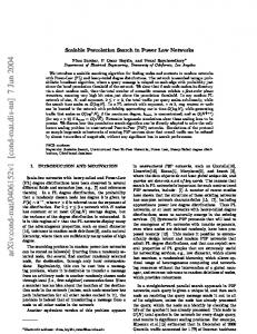
only for a discrete set of points, namely for the vertices of the road network. Thus, we have to fill the gaps by deciding how the isocontour should pass through the regions between the roads. The fact that the quality of the resulting visualization heavily depends on these decisions makes computing isocontours in road networks an interesting algorithmic problem. Formally, we consider the road network to be given as a directed graph G = (V, E), along with vertex positions in the plane and two weight functions len : E → R+ and cons : E → R representing length and resource consumption, respectively. For a source vertex s ∈ V and a range r ∈ R≥0 , a vertex v belongs to the reachable subgraph if the shortest path from s to v has a total resource consumption of at most r, i.e., shortest paths are computed according to the length, while reachability is determined by the consumption. Coming back to our initial question concerning the electric vehicle, the source vertex is the initial position, the range is the current state of charge, the length corresponds to travel time, and energy is the resource consumed on edges. We allow negative resource consumption to take account of recuperation, which enables electric vehicles to recharge their battery when braking. Note that our setting is sufficiently general to allow for other applications. By setting the length as well as the resource consumption of edges to the travel time (len ≡ cons), one obtains the special case of isochrones. There is a wide range of applications for isochrones, including reachability analyses [2, 14, 13], geomarketing [11], and various online applications [24]. Known approaches focus on isochrones of small or medium range. But isochrones can be useful in more challenging scenarios, for example, to visualize the area reachable by a truck driver within a day of work. This motivates our work on fast isocontour visualization. Our algorithms for computing isocontours in road networks are guided by three major objectives. The isocontours must be exact in the sense that they correctly separate the reachable subgraph from the remaining unreachable subgraph; the isocontours should be polygons of low complexity (i. e., consist of few segments, enabling efficient rendering and a clear, uncluttered visualization); and the algorithms should be sufficiently fast in practice for interactive applications, even on large inputs of continental scale. Figure 1 shows an example of isocontours visualizing the range of an electric vehicle. The left figure depicts a polygon that closely resembles the output of isocontour algorithms considered state-of-the-art in recent works [11, 25]. Unfortunately, the number of segments becomes quite large even in this medium-range example (more than 10 000 segments). The figure to the right shows the result of our approach presented in Section 5.3, which contains the same reachable subgraph while using 416 segments in total. Related Work. Several existing algorithms consider the problem of computing the subnetwork that is reachable within a given timespan. The MINE algorithm [14] is a search to compute isochrones in transportation networks based on Dijkstra’s well-known algorithm [8]. An improved variant, called MINEX [13], reduces space requirements. Both approaches work on spatial databases, prohibiting interactive applications (having running times in the order of minutes for large ranges). To enable much faster shortest-path queries in practice, speedup techniques [1] seperate the workflow into an offline preprocess-

2

(a)

(b)

Figure 1: Real-world example of isocontours in a mountainous area (near Bern, Switzerland). Both figures visualize range of an electric vehicle positioned at the black disk with a state of charge of 2 kWh. Note that the polygons representing the isocontour contain holes, due to unreachable high-ground areas. (a) The isocontour computed by the approach in Section 5.1, which resembles previous works [25]. (b) The result of one of our new approaches, presented in Section 5.3. ing phase and an online query phase. Recently, some speedup techniques were extended to the isochrone scenario [3, 12], enabling query times in the order of milliseconds. Yet, these approaches only deal with the computation of the reachable subgraph, rather than visualization of isocontours. Regarding isocontour visualization, efficient approaches exist for shape characterization of point sets, such as α-shapes [10] or χ-shapes [9]. However, we are interested in separating subgraphs rather than point sets. Marciuska and Gamper [25] present two approaches to visualize isochrones. The first transforms a given reachable network into an isochrone area by simply drawing a buffer around all edges in range. The second one creates a polygon without holes, induced by the edges on the boundary of the embedded reachable subgraph. Both approaches were implemented on top of databases, providing running times that are too slow for many applications (several seconds for small and medium ranges). Gandhi et al. [15] introduce an algorithm to approximate isocontours in sensor networks with provable error bounds. They preserve the topological structure of the given family of contours, forbidding intersections. Finally, there are different works presenting applications which make use of isocontours in the context of urban planning [2], geomarketing with integrated traffic information [11], and range visualization for electric vehicles [18].

3

Contribution and Outline. We propose algorithms for efficiently computing polygons representing isocontours in road networks. All approaches compute isocontours that are exact, i. e., they contain exactly the subgraph reachable within the given resource limit, while having low descriptive complexity. Efficient performance of our techniques is both proven in theory and demonstrated in practice on realistic instances. In Section 2, we formalize the notion of reachable and unreachable subgraphs. Moreover, we state the precise problem and outline our algorithmic approach to solve it. Section 3 attacks the first resulting subproblem of computing border regions, that is, polygons that represent the boundaries of the reachable and unreachable subgraph. An isocontour must separate these boundaries. In Section 4, we consider the special case of separating two hole-free polygons with a polygon with minimum number of segments. While this problem can be solved in O(n log n) time [28], we propose a simpler algorithm that uses at most two additional segments, runs in linear time, and requires a single run of a minimum-link path algorithm. We also propose a minimum-link path algorithm that is simpler than a previous approach [26]. Section 5 extends these results to the general case, where border regions may consist of more than two components. Since the complexity of the resulting problem is unknown, we focus on efficient heuristic approaches that work well in practice, but do not give guarantees on the complexity of the resulting range polygons. Section 6 contains our extensive experimental evaluation using a large, realistic input instance. It demonstrates that all approaches are fast enough even for use in interactive applications. We close with final remarks in Section 7.

2 Problem Statement and General Approach Let G = (V, E) be a road network, which we consider as a geometric network where vertices have a fixed position in the plane and edges are represented by straight-line segments between their endpoints. A source s ∈ V and a maximum range r together partition the network into two parts, one that is within range r ∈ R≥0 from v, and the part that is not. An isocontour separates these two parts. We are interested in visualizing such isocontours efficiently. In the following, we give a precise definition of the (un)reachable parts of the network and formally define range polygons, which we use to represent isocontours. Range Polygons. A path π in G starting at s is passable if the consumption of π, i. e., the sum of its edge consumption values, is at most r. A vertex v is reachable (with respect to the maximum range r) if the shortest s–v-path is passable. A vertex that is not reachable is unreachable. For edges the situation is more complicated. We partition the edges into four types, namely unreachable edges, boundary edges, accessible edges, and passable edges. Figure 2 shows an example of the different edge types. If both endpoints of an edge (u, v) are unreachable, then also the edge (u, v) is unreachable. If exactly one endpoint is reachable, then (u, v) is not part of the reachable network, and we call it boundary edge. However, the fact that both u and v are reachable does not necessarily imply that (u, v) is part of the

4

Figure 2: Graph with reachable (white) and unreachable (black) vertices. Black edges are passable. Dashed edges are boundary edges if they have an unreachable endpoint, and accessible if both endpoints are reachable. Gray edges are unreachable. reachable network. Let πu and πv denote the shortest paths from s to u and v, respectively. If the resource consumptions of πu and πv do not allow the traversal of the edge (u, v) in either direction, i.e., cons(πu ) + cons((u, v)) > r and cons(πv ) + cons((v, u)) > r, then we do not consider (u, v) as reachable. Since we can reach both endpoints of (u, v), we call it accessible. Otherwise, the edge can be traversed in at least one direction, so it is passable. Let Vr be the reachable vertices and let Vu = V \Vr be the unreachable vertices. Similarly, let Eu , Eb , Ea , Er denote the set of unreachable edges, boundary edges, accessible edges, and passable edges, respectively. Note that for arbitrary pairs of edges (u, v) and (v, u), both edges belong to the same set. The reachable part of the network is Gr = (Vr , Er ), and the unreachable part is Gu = (Vu , Eu ). A range polygon is a plane (not necessarily simple) polygon P separating Gr and Gu in the sense that its interior contains Gr and has empty intersection with Gu . Note that every range polygon P intersects each boundary edge an odd number of times and each accessible edge an even number of times. In particular, an accessible edge may be totally or partially contained in the interior of a range polygon. If the input graph G is planar, one can construct a range polygon by slightly shrinking the faces of the subgraph induced by all reachable vertices, though this may produce many holes; see the shaded area in Figure 2. However, if G is not planar, a range polygon may not even exist. If a passable edge intersects an unreachable edge, the requirements of including the passable and excluding the unreachable edge obviously contradict. To resolve this issue, we consider the planarization Gp of G, which is obtained from G by considering each intersection point p as a dummy vertex that subdivides all edges of G that contain p. We transfer the above partition of G into reachable and unreachable parts to Gp as follows. A dummy vertex is reachable if and only if it subdivides at least one passable edge of the original graph. As above, an edge of Gp is unreachable if both endpoints are unreachable, and it is a boundary edge if exactly one endpoint is reachable. If both endpoints are reachable, it is accessible (passable) if and only if the edge in G containing it is accessible (passable). Clearly, after the planarization, a range polygon always exists. Figure 3 shows different cases of crossing edges. Note that this way of handling crossings ensures that a range polygon for Gp contains the reachable vertices of G and excludes the unreachable vertices of G. However, unreachable edges of G may be partially contained in the range

5

(a)

(b)

(c)

(d)

Figure 3: (a) Intersection of a passable and an unreachable edge, the dummy vertex is reachable. (b) Intersection of an accessible and an unreachable edge. The dummy vertex is unreachable, dashed edges become boundary edges. (c) Intersection of an unreachable edge and a boundary edge, creating an unreachable dummy edge and a new boundary edge replacing the original one. (d) An intersection of accessible edge creates an unreachable dummy vertex and four new boundary edges. polygon if they cross passable edges. Finally, to avoid special cases, we add a bounding box of dummy vertices and edges to Gp , connecting each vertex in the bounding box to its respective closest vertex in Gp with an edge of infinite length. Thereby, we ensure that neither the reachable nor the unreachable subgraph is empty, as the reachable (unreachable) subgraph contains at least the source (the bounding box). General Approach. We seek to compute a range polygon with respect to the planarized graph Gp that has the minimum number of holes, and among these we seek to minimize the complexity of the range polygon, i. e., its number of segments. We note that using Gp may require more holes than G (see also Figure 3d), but guarantees the existence of a solution. Consider the graph G0 consisting of the union of the reachable and the unreachable graph. Clearly, all segments of the range polygon lie in faces of G0 . A face of G0 that is incident to both reachable and unreachable components is called border region. Since a range polygon separates the reachable and unreachable parts, each border region contains at least one connected component of a range polygon. Therefore, the number of border regions is a lower bound on the number of holes. On the other hand, components in faces that are not border regions can be removed and several connected components in the same border region can always be merged, potentially at the cost of increasing the complexity; see Figure 4. Therefore, a range polygon with the minimum number of holes (with respect to Gp ) can be computed as follows. 1. Compute the reachable and unreachable parts of G. 2. Planarize G, compute the reachable and unreachable parts of the planarization Gp . 3. Compute the border regions. 4. For each border region B, compute a simple polygon of minimum complexity that is contained in B and separates the unreachable components incident to B from the reachable component. In the following sections we discuss several alternative implementations for these steps. The first three steps are described together in Section 3. The main part of the paper is concerned with Step 4. Each connected component of the boundary of a border region is a hole-free

6

(a)

(b)

(c)

Figure 4: (a) A hole of the range polygon that contains no unreachable vertices can always be removed. (b) Two holes that can be merged into one as they lie in the same border region. (c) These two holes cannot be merged as they are separated by passable edges. non-crossing polygon. Note that these polygons are not necessarily simple in the sense that they may contain the same segment twice in different directions; see Figure 5. Thus, each border region is defined by two sets R and U of hole-free non-crossing polygons, where R contains the boundaries of the reachable components and U contains the boundaries of the unreachable components. For our range polygon, we seek a simple polygon with the minimum number of links that separates U from R. This problem has been previously studied. Guibas et al. [21] showed that the problem is NP-complete in general. In our case, however, it is |R| = 1 since the reachable part of the network is, by definition, connected. Guibas et al. [21] left this case as an open problem, and, to the best of our knowledge, it has not been resolved. In Section 4, we first consider border regions that are incident to only one unreachable components, i.e., |R| = |U | = 1. In this case, a polygon with the minimum number of segments that separates R and U can be found in O(n log n) time (where n is the total number of segments in the border region) using the algorithm of Wang [28]. However, this algorithm is rather involved, as it requires a (constant) number of calls of a minimum-link path algorithm. Instead, we propose a simpler algorithm that uses at most two more segments than the optimum, runs in linear time, and relies on a single call of a minimum-link path algorithm. In addition, we give a new linear minimum link path algorithm that is simpler than previous algorithms for this problem. In Section 5, we consider the general case of our problem, where a border region may be incident to more than one unreachable component. We propose several algorithms for this problem. As mentioned above, the complexity of this problem is unknown, and we therefore focus on efficient heuristic approaches that work well in practice but do not necessarily give provable guarantees on the number of segments.

7

U3 U2 U1 R U4

Figure 5: An example of a border region where the set U consists of several unreachable components with boundaries U1 , U2 , U3 and U4 . Shaded areas show the reachable (dark gray) and unreachable (light gray) part with boundaries R and U of G, respectively. The white area represents the border region.

3 Computing the Border Regions We describe an algorithm to compute the reachable and unreachable part of the input graph G = (V, E), the planarization of these parts, and extraction of all border regions. We modify Dijkstra’s algorithm [8] to compute the reachable and unreachable parts in time O(|V | log |V |), given that |E| ∈ O(|V |) for graphs representing road networks. Afterwards, we map this information to the planarized graph Gp in O(|E|) time. Finally, we extract the border regions by traversing all faces of the planar graph that contain at least one boundary edge or accessible edge, which requires linear time in the size of all border regions. Below, we discuss efficient implementations of these three steps. First, we describe a variant of Dijkstra’s algorithm that computes, for a given source vertex s and a range r ∈ R≥0 • for each vertex v ∈ V , whether v is reachable from s; • the set Ex := Eb ∪ Ea of all boundary edges and accessible edges; • for every edge (u, v) ∈ E \ Ex , whether (u, v) is passable or unreachable. For the sake of simplicity, we assume that shortest paths are unique (wrt. the length function). Thereby, we avoid the special case of two paths with equal distance but different consumption, which requires additional tie breaking. The algorithm works as follows. Along the lines of Dijkstra’s algorithm, it maintains vertex labels consisting of (tentative) values for distance d(·) and resource consumption c(·), both initially set to 0 for s and ∞ for all other vertices. The algorithm uses a priority queue of vertices, initially containing s. In each step, it extracts the vertex u with minimum distance label from the queue, thereby settling it. Then, all outgoing edges (u, v) are scanned, checking whether d(u) + len(u, v) < d(v). If this is the case, the labels at v are updated accordingly to d(v) := d(u) + len(u, v) and c(v) := c(u) + cons(u, v). Also, v is inserted into the queue if it is not contained already.

8

Once the queue runs empty, we know that a vertex v ∈ V is reachable if and only if c(v) ≤ r. An edge (u, v) ∈ E \ Ex is passable if u (and thus, also v) is reachable, and it is unreachable otherwise. Correctness follows directly from the correctness of Dijktra’s algorithm and the fact that we simply sum up consumption values along shortest paths. We describe how to compute the set Ex of boundary edges and accessible edges, i. e., all edges that intersect the interior of the border regions, which are required as input for later steps. A naïve approach could run a linear sweep over all edges after the search terminates. In practice, we can do better by computing Ex on-the-fly (especially when the stopping criterion described below is applied). We know whether an edge (u, v) belongs to Ex as soon as both u and v were settled (and thus have final labels). Therefore, after extracting a vertex from the queue, we check all incident edges and add them to Ex if the respective neighbor was settled and one of the following conditions holds. Either, exactly one endpoint of the edge is currently reachable, or both endpoints are reachable but the edge is not passable, i. e., c(u) + cons((u, v)) > r and c(v) + cons((v, u)) > r if (v, u) ∈ E. Stopping Criterion. Without further modification, the described algorithm settles all vertices in the graph (presuming it is strongly connected). In practice, this may be undesirable, especially for small ranges. However, simply pruning the search at unreachable vertices does not preserve correctness. Assume we do not insert an unreachable vertex u into the queue. Consider another unreachable vertex v, such that the shortest s–v-path contains u. There might exist some (non-shortest) path from s to v with lower resource consumption that is found by the algorithm instead. Then, v is falsely identified as reachable. However, we can safely abort the query as soon as no reachable vertex is left in the queue, since no reachable vertex can be found from an unreachable vertex (in case of negative consumption values, we presume that battery constraints apply [4]). To efficiently check whether this stopping criterion is fulfilled, we simply maintain a counter to keep track of the number of reachable vertices in the queue. Using the stopping criterion, we may not have found all boundary edges once the search terminates, as possibly not all unreachable endpoints of boundary edges have been settled. However, we know that the unreachable endpoint v of missing boundary edges (u, v) must have been added to the queue when u was settled. We ensure that unreachable vertices u of boundary edges (u, v) are in the queue as well, by scanning incident incoming edges when settling the reachable vertex u and adding each neighbor to the queue with key ∞ if it is not contained yet. We obtain the remaining boundary edges in a sweep over all vertices left in the queue, checking for each its incident edges. Even with the stopping criterion in place, the running time is impractical on large inputs. Speedup techniques [1] are a common approach for much faster queries in practice. A recent work [3] presents techniques extending the basic approach described above that enable fast computation of boundary edges (considering the special case of len ≡ cons). Since they can be adapted to our scenario, we focus on the remaining steps for computing range polygons.

9

Planarization. We planarize G in a preprocessing step to obtain Gp = (Vp , Ep ). This can be done using the well-known sweep line algorithm [5, 7]. For each vertex in Gp , we store its original vertex in G (if it exists). In practice, where vertices are represented by indices {1, . . . , |V |}, this mapping can be done implicitly since Vp is a superset of V . After computing the reachable subgraph of G as described above, we compute reachability of dummy vertices and the set Ex of boundary edges and accessible edges in Gp as follows. First, we have to ensure that boundary edges and accessible edges returned by the algorithm are actually contained in Gp . We add a flag to all edges in G during preprocessing that indicates whether an edge is contained in Gp . Then, we modify our search algorithm to add edges to Ex only if this flag is set. After the search terminates, we check for each dummy vertex v ∈ Vp whether it is reachable, by checking passability of all original edges in E that contain v. To this end, we precompute an array of all original edges that were split during planarization, and for each split edge a list of dummy vertices it contains (an original edge may intersect several other edges). Then, we can sweep over this array of edges, and for each passable edge, we mark all its dummy vertices as reachable. Finally, we perform a sweep over all edges in Gp that have at least one dummy vertex as endpoint, to determine any missing edges in Ex (to test whether an edge is accessible, we need a pointer to the unique original edge containing it). Note that the linear sweep steps produce limited overhead in practice, since the number of dummy vertices in graphs representing road networks is typically small (as large parts of the input are planar to begin with). Afterwards, a vertex in Vp is reachable if it is a dummy vertex marked as reachable, or its corresponding original vertex is reachable (if it exists). Otherwise, it is unreachable. For edges in Ep \ Ex , we check reachability of their endpoints to determine whether they are passable or unreachable. An alternative approach modifies the search algorithm to work directly on the planar graph Gp to avoid the additional linear sweeps. However, this produces overhead during the search (e. g., case distinctions for dummy vertices). Consequently, such approaches did not provide significant speedup in preliminary experiments. Moreover, determining the reachable subgraph of Gp in a separate step simplifies the integration of speedup techniques for the more expensive search algorithm [3]. Extracting the Border Regions. Given the set Ex of boundary edges and accessible edges in Gp , we describe how to compute the actual border regions (i. e., the polygons describing R and U ). The basic idea is to traverse all faces of Gp that contain edges in Ex , to collect the segments that form boundaries of the border regions. Clearly, all passable edges in these faces are part of some reachable boundary, while all unreachable edges belong to an unreachable boundary. Moreover, since Gp is strongly connected, all faces contained in a border region must contain an edge in Ex . Thus, traversing these faces is sufficient to obtain all border regions. In somewhat more detail, we maintain two flags for every edge (u, v) in Ex indicating whether u or v has been visited, respectively, initially set to false. Let (u, v) be the first edge

10

v

f3

f4

u f1

v

f3

f5 w x

f2 f1 u

f4

f2

f5

y

(a)

(b)

Figure 6: Visited edges (green) when extracting a reachable boundary. (a) Starting at the boundary edge (u, v) ∈ Ex , the face f1 is traversed first until the boundary edge (x, y) ∈ Ex is encountered. Afterwards, the faces f2 , f3 , f4 , f3 , f5 are visited in this order until (u, v) is reached again. (b) Starting at the accessible edge (u, v) ∈ Ex , the face f1 is traversed until (v, u) ∈ Ex is reached. Then, the faces f2 , f3 , f4 , f5 , f2 are processed before (u, v) is reached again. of Ex that is considered, and without loss of generality, let u be reachable. We compute the (unique) reachable component R(u,v) of the border region B(u,v) containing (u, v); see Figure 6. We mark (u, v) as visited and traverse the face left of (u, v), following the unique neighbor w of u in this face that is not v. Every edge that we traverse is added to R(u,v) . As soon as we encounter an edge (x, y) ∈ Ex , we continue by traversing the twin face of (x, y), i. e., the unique face of Gp that contains the other side of (x, y). The edge (x, y) itself is not added to R(u,v) . Moreover, we mark (x, y) as visited. The current extraction step is finished as soon as (u, v) with the same orientation is reached again; see Figure 6. If v is unreachable, (u, v) is a boundary edge. Thus, we continue with the extraction of the unreachable component U(u,v) containing v in the same manner and assign it to B(u,v) . We loop over the remaining edges in Ex and extract boundaries corresponding to vertices not visited before. By extracting reachable components first, we ensure that the corresponding reachable boundary of some unreachable component is always known before extraction, namely, the boundary containing the reachable endpoint of the considered edge in Ex . Therefore, the unreachable component is assigned to the unique border region that contains this reachable boundary. Implementation Details. To extract the components of all border regions, we have to traverse the faces of the planar input graph. We use a cache-friendly data structure to represent these faces, allowing us to run along a face efficiently. For each face, we store the sequence of vertices as they are found traversing the face in clockwise order starting at an arbitrary vertex. At the beginning and at the end of this sequence, we store sentinels that hold the index of the first and last entry of a vertex of the corresponding face, respectively. Then, we can use one single array that holds all faces of the graph. Traversing the face in either direction requires only a sweep, jumping at most once to the beginning or end of

11

e

e

R

R

U

U

(a)

(b)

Figure 7: (a) The polygon S (red) separating R and U with OPT = 3 links. (b) The polygon S 0 obtained by a minimum-link path from e has OPT + 2 = 5 segments. the face, respectively. For consecutive vertices u, v in this array, we store at v its index in the corresponding twin face of the edge (u, v). Finally, we store for every edge (u, v) in the graph the two indices of the head vertex v in this data structure, i. e., its occurrence in the faces left and right of this edge. To efficiently decide whether an edge is in Ex , or if an edge in Ex was marked as visited, we store this list as an array and sort it (e. g., by the index of the head vertex) before extracting the reachable components. Then we can quickly retrieve an edge in this array using binary search (we also tried using hash sets as an alternative approach, but this turned out to be slightly slower in preliminary experiments).

4 Range Polygons in Border Regions Without Holes Given a border region B with reachable component R and a single unreachable component U , we present an algorithm for computing a polygon that separates R and U . In Section 5, we describe how to generalize our approach to the case |U | > 1. The basic idea is to add an arbitrary boundary edge e to B, thereby connecting both components R and U . Since we presume that G is strongly connected, such a boundary edge always exists. In the resulting hole-free non-crossing polygon B 0 , we compute a path with minimum number of segments that connects both sides of e. The algorithm of Suri [26] computes such a minimum-link path π 0 in linear time. We obtain a separating polygon S 0 by connecting the endpoints of π 0 along e. It is easy to see that this yields a polygon with at most two additional segments compared to an optimal solution. Lemma 1. Let S be a polygon that separates R and U with minimum number of segments, and let OPT denote this number. Then S 0 has at most OPT + 2 segments. Proof. We can split S at e into a path π connecting both sides of e. Clearly, π has at most OPT+1 links (if a segment of S crosses e, we split it into two segments with endpoints in e; see Figure 7). Since π 0 is a minimum-link path, we have |π 0 | ≤ |π| = OPT + 1. Moreover, S 0 is obtained by adding a single subsegment of e to π 0 , so its complexity is bounded by OPT + 2.

12

t6

t7

t8

t9

t10

b

0 w(a) P

b

`(b6 )

b6

t5

t4 t3 t2

b8

r(b6 ) π6r

π8`

π6` t1 a

a

(a)

(b)

`(a) a

r(a)

π8r

a

(c)

Figure 8: (a) The important triangles (with respect to a and b) of a polygon. (b) The window w(a) is an edge of the (shaded) visibility polygon. (c) The left and right shortest paths (blue) intersect for i = 8 but not for i = 6. We now address the subproblem of computing a minimum-link path between two edges of a simple polygon. The linear-time algorithm of Suri [26] starts by triangulating the input polygon. To save running time, we can preprocess this step and triangulate all faces of the planar graph Gp . Afterwards, in each step of Suri’s algorithm, a window (which we formally define in a moment) is computed. To obtain the windows in linear time, it relies on several calls to a subroutine computing visibility polygons. While this is sufficient to prove linear running time, it seems wasteful from a practical point of view. In the following, we present an alternative algorithm for computing the windows that also results in linear running time, but is much simpler. It can be seen as a generalization of an algorithm by Imai and Iri [23] for approximating piecewise linear functions. Windows and Visibility. Let P be a simple polygon and let a and b be edges of P . We want to compute a minimum-link polygonal path starting at a and ending in b that lies in the interior of P . Let T be the graph obtained by arbitrarily triangulating P . Let ta and tb be the triangles incident to a and b, respectively. As T is an outerplanar graph, its (weak) dual graph has a unique path ta = t1 , t2 , . . . , tk−1 , tk = tb from ta to tb ; see Figure 8a. We call the triangles on this path important and their position in the path their index. The visibility polygon V (a) of the edge a in P is the polygon that contains a point p in its interior if and only if there is a point q on a such that the line segment pq lies inside P . Let i be the highest index such that the intersection of the triangle ti with the visibility polygon V (a) is not empty. The window w(a) is the edge of V (a) that intersects ti closest to the edge between ti and ti+1 ; see Figure 8b. Note that w(a) separates the polygon P into two parts. Let P 0 be the part containing the edge b that we want to reach. A minimumlink path from a to b in P can then be obtained by adding an edge from a to w(a) to a minimum-link path from w(a) to b in P 0 . Thus, the next window is computed in P 0 starting with the previous window w(a). In the following, we first describe how to compute the first window and then discuss what has to be changed to compute the subsequent windows. Let Ti be the subgraph of T induced by the triangles t1 , . . . , ti and let Pi be the polygon bounding the outer face of Ti . The polygon Pi has two special edges, namely a and the

13

`(bi )

λ`i

ti+1 y

ti

r(bi )

ti+1 y

λri

ti

λ`i = λri bi

πir

πi`

x

x

a

r(a)

`(a) (a)

(b)

(c)

Figure 9: (a) The shortest path from r(a) to `(bi ) consists of the bold prefix of πir , the red segment, and the bold suffix of πi` . (b) The two visibility lines spanning the (shaded) visibility cone. (c) Degenerated case. edge shared by ti and ti+1 , which we call bi . Let `(a) and r(a), and `(bi ) and r(bi ) be the endpoints of a and bi , respectively, such that their clockwise order is r(a), `(a), `(bi ), r(bi ) (think of `(·) and r(·) being the left and right endpoints, respectively); see Figure 8c. We define the left shortest path πi` to be the shortest polygonal path (shortest in terms of Euclidean length) that connects `(a) with `(bi ) and lies inside or on the boundary of Pi . The right shortest path πir is defined analogously for r(a) and r(bi ); see Figure 8c. Assume that the edge bi is visible from a, i.e., there exists a line segment in the interior of Pi that starts at a and ends at bi . Such a visibility line separates the polygon into a left and a right part. Observe that it follows from the triangle inequality that the left shortest path πi` and the right shortest path πir lie inside the left and right part, respectively. Thus, these two paths do not intersect. Moreover, the two shortest paths are outward convex in the sense that the left shortest paths πi` has only left bends when traversing it from `(a) to `(bi ) (the symmetric property holds for πir ); see the case i = 6 in Figure 8c. We note that the outward convex paths are sometimes also called “inward convex” and the polygon consisting of the two outward convex paths together with the edges a and bi is also called hourglass [19]. The following lemma, which is similar to a statement shown by Guibas et al. [20, Lemma 3.1], summarizes the above observation. Lemma 2. If the triangle ti is visible from a, then the left and right shortest paths in Pi−1 have empty intersection. Moreover, if these paths do not intersect, they are outward convex. Guibas et al. [20] argue that the converse of the first statement is also true, i.e., if the two paths have empty intersection, then the triangle ti+1 is visible from a. Their main arguments go as follows. The shortest path (wrt. Euclidean length) in the hourglass that connects r(a) with `(bi ) is the concatenation of a prefix of πir , a line segment from a vertex x of πir to a vertex y of πi` , and a suffix of πi` ; see Figure 9a. We call the straight line through x and y the left visibility line and denote it by λ`i . We assume λ`i to be oriented from x to y and call x and y the source and target of λ`i . Analogously, one can define the

14

λ`i−1

`(bi )

λ`i

λri

bi

t i bi

r πi−1

πir

ti ` πi−1

λri−1

λri−1 λ`i−1 `(bi ) bi ti r πi−1

` πi−1

λ`i

λri ti

bi

πi`

πir

λ`i−1

λri−1 `(bi ) t i bi

w(a) ti

bi

r ` πi−1 πi−1

πi` a (a)

a (b)

a

a (d)

(c)

a (e)

a (f)

Figure 10: (a) The new vertex `(bi ) lies in the visibility cone. (b) The updated left shortest path πi` and left visibility line λ`i . (c) The vertex `(bi ) lies to the left of λ`i−1 . (d) The left shortest path has to be updated, the left visibility line remains unchanged. (e) The vertex `(bi ) lies to the right of λri−1 , i.e., ti+1 is not visible from a. (f) The window w(a) is a segment of λri−1 . right visibility line λri ; see Figure 9b. We call the intersection of the half-plane to the right of λ`i with the half-plane to the left of λri the visibility cone. It follows that the intersection of the visibility cone with the edge bi is not empty and a point on the edge bi is visible from a if and only if it lies in this intersection [20]. This directly extends to the following lemma. Lemma 3. If the left and right shortest paths in Pi−1 have empty intersection, ti is visible from a. Moreover, a point in ti is visible from a if and only if it lies in the visibility cone. Note that when πir and πi` are both outward convex and intersect, the visibility cone degenerates to a line; see Figure 9c. For the sake of simplicity, we presume that all points are in general position, which prevents this special case. (In practice, it is handled implicitly by the implementation of Line 4 in Algorithm 1 below.) The above observations then justify the following approach for computing the window. We iteratively increase i until the left and the right shortest path of the polygon Pi intersect. We then know that the triangle ti+1 is no longer visible; see Lemma 2. Moreover, as the left and the right shortest paths did not intersect in Pi−1 , the triangle ti is visible from a; see Lemma 3. To find the window, it remains to find the edge of the visibility polygon V (a) that intersects ti closest to the edge between ti and ti+1 . Thus, by the second statement of Lemma 3, the window must be a segment of one of the two visibility lines. It remains to fill out the details of this algorithm, argue that it runs in overall linear time, and describe what has to be done in later steps, when we start at a window instead of an edge. Computing the First Window. We start with the details of the algorithm starting from ` an edge; also see Algorithm 1. Assume the triangle ti is still visible from a, i.e., πi−1 and r πi−1 do not intersect. Assume further that we have computed the left and right shortest ` r paths πi−1 and πi−1 as well as the corresponding visibility lines λ`i−1 and λri−1 in a previous step. Assume without loss of generality that the three corners of the triangle ti are `(bi−1 ),

15

Algorithm 1: Computes the first window w(a). 1 2 3

4 5 6

7 8 9

10 11 12 13 14

// initial paths (one-vertex sequences) and visibility lines π ` = [`(a)]; π r = [r(a)]; λ` = line(r(a), `(a)); λr = line(`(a), r(a)) for i = 1 to k do if r(bi ) = r(bi−1 ) then // bi not visible ⇒ return window if `(bi ) lies to the right of λr then x = first intersection of λr with P after target(λr ) return segment(target(λr ), x) // extend left path π ` like in Graham’s scan append `(bi ) to π ` while last bend of π ` is a right bend do remove second to last element from π ` // `(bi ) in visibility cone ⇒ update left visibility line λ` if `(bi ) lies to the right of λ` then target(λ` ) = `(bi ) while λ` is not a tangent of π r at source(λ` ) do source(λ` ) = successor of source(λ` ) in π r else // case `(bi ) = `(bi−1 ) is symmetric to above case r(bi ) = r(bi−1 )

`(bi ), and r(bi ) = r(bi−1 ). There are three possibilities shown in Figure 10, i.e., the new vertex `(bi ) lies either in the visibility cone spanned by λ`i−1 and λri−1 , to the left of the left visibility line λ`i−1 , or to the right of the right visibility line λri−1 . By Lemma 3, a point in ti is visible from a if and only if it lies inside the visibility cone. Thus, the edge bi between ti and ti+1 is no longer visible if and only if the new vertex `(bi ) lies to the right of λri−1 ; see Figure 10e. In this case, we can stop and the desired window r w(a) is the segment of λri−1 starting at its touching point with πi−1 and ending at its first intersection with an edge of P ; see Figure 10f and lines 4–6 of Algorithm 1. In the other two cases (Figure 10a and Figure 10c), we have to compute the new left and right shortest paths πi` and πir and the new visibility lines λ`i and λri (Figure 10b and r Figure 10d). Note that the old and new right shortest paths πi−1 and πir connect the same endpoints r(a) and r(bi−1 ) = r(bi ). As the path cannot become shorter by going through r . The same argument shows that λr = λr the new triangle ti , we have πir = πi−1 i−1 (recall i that the visibility lines were defined using a shortest path from `(a) to r(bi−1 ) = r(bi )). We compute the new left shortest path πi` as follows; see Lines 7–9 of Algorithm 1. Let ` ` x be the latest vertex on πi−1 such that the prefix of πi−1 ending at x concatenated with the segment from x to `(bi ) is outward convex. We claim that πi` is the path obtained by this concatenation, i.e., this path lies inside Pi and there is no shorter path lying inside Pi .

16

λ`i−1 `(bi−1 )

`(bi ) `(bi−1 )

y

λ`i

λ`i

`(bi ) `(bi−1 )

y

x r(a) (a)

x0 x

x r(a) (b)

r(a) (c)

Figure 11: (a) The shortest path from r(a) to `(bi−1 ) (bold) defining the left visibility line λ`i−1 . (b) The visibility line does not change if `(bi ) lies to the left of λ`i−1 . (c) Illustration how the visibility line changes when `(bi ) lies to the right of λ`i−1 . It follows by the outward convexity, that there cannot be a shorter path inside Pi from ` `(a) to `(bi ). Moreover, by the assumption that πi−1 was the correct left shortest path in Pi−1 , the subpath from `(a) to x lies inside Pi . Assume for contradiction that the new segment from x to `(bi ) does not lie entirely inside Pi . Then it has to intersect the right shortest path and it follows that the right shortest path and the correct left shortest path have non-empty intersection, which is not true by Lemma 2. To get the new left visibility line λ`i , we have to consider the shortest path in Pi that connects r(a) with `(bi ). Let x and y be the source and target of λ`i−1 , respectively, i.e., the shortest path from r(a) to `(bi−1 ) is as shown in Figure 11a. If the new vertex `(bi ) lies to the left of λ`i−1 (Figure 11b), then the shortest path from r(a) to `(bi ) also includes the segment from x to y. Thus, λ`i = λ`i−1 holds in this case. Assume the new vertex `(bi ) lies to the right of λ`i−1 (Figure 11c). Let x0 be the latest vertex on the path πir such that the concatenation of the subpath from r(a) to x0 with the segment from x0 to the new vertex `(bi ) is outward convex in the sense that it has only right bends; see Figure 11c. We claim that this path lies inside Pi and that there is no shorter path inside Pi . Moreover, we claim r that x0 is either a successor of x in πi−1 or x0 = x. Clearly, the concatenation of the path from r(a) to x with the segment from x to `(bi ) is outward convex, thus the latter claim follows. It follows that the segment from x0 to `(bi ) lies to the right of the old visibility ` lies line λ`i−1 . Thus, it cannot intersect the path πi` (except in its endpoint `(bi )), as πi−1 ` 0 r to the left of λi−1 . Moreover, as we chose x to be the last vertex on πi−1 with the above property, this new segment does not intersect πir (except in x0 ). Hence, the segment from x0 to `(bi ) lies inside Pi . As before, it follows from the convexity that there is no shorter path inside Pi . Thus, λ`i is the line through x0 and `(bi ) (x0 is the new source and `(bi ) is the new target). It follows that Lines 10–13 correctly compute the new left visibility line. Lemma 4. Let th be the triangle with the highest index that is visible from a. Then Algorithm 1 computes the first window w(a) in O(h) time.

17

π0` b

λ`0

th 0

a

v2 v3 v4 v5 v6

v1

a00

bh

bh bh

0

a

π0r (a)

0

0

a

λr0

a (c)

(b)

(d)

Figure 12: (a) The polygon P 0 we are interested in after computing the first window a0 . The initial part P00 is shaded yellow. (b) Initial left and right shortest paths π0` and π0r (blue) with corresponding visibility lines (red). (c) The sequence v1 , . . . , v6 we use for Graham’s scan. Triangles of P intersected by a0 are shaded yellow. (d) Computing the shortest path from `(a00 ) = `(a0 ) to `(bh ) in this subdivided polygon using Algorithm 1 actually applies Graham’s scan to v1 , . . . , v6 . Proof. We already argued that Algorithm 1 correctly computes the first window. To show that it runs in O(h) time, first note that the polygon Ph has linear size in O(h). Thus, it suffices to argue that the running time is linear in the size of Ph . In each step i, we first check whether the next triangle is still visible by testing whether the new vertex `(bi ) (or r(bi )) lies to the right of the visibility line λri−1 (or to the left of λ`i−1 ). This takes only constant time. When updating the left and right shortest paths, we have to iteratively remove the last vertex of the previous path until the resulting path is outward convex. This takes time linear in the number of vertices we remove. However, a vertex removed in this way will never be part of a left or right shortest path again. Thus, the number of these removal operations over all h steps is bounded by the size of Ph . When updating the visibility lines, the only operation potentially consuming more than constant time is finding the new source x0 . As x0 is a successor of the previous source x (or x0 = x), we never visit a vertex of Ph twice in this type of operation. Thus, the total running time of finding these successors over all h steps is again linear in the size of Ph . Initialization for Subsequent Windows. As mentioned before, the first window w(a) we compute separates P into two smaller polygons. Let P 0 be the part including the edge b (and not a). In the following, we denote w(a) by a0 . To get the next window w(a0 ), we have to apply the above procedure to P 0 starting with a0 . However, this would require to partially retriangulate the polygon P 0 . More precisely, let th be the triangle with the highest index that is visible from a and let bh be the edge between th and th+1 ; see Figure 12a. Then bh separates P 0 into an initial part P00 (the shaded part in Figure 12a) and the rest (having b on its boundary). The latter part is properly triangulated, however, the initial part P00 is not. The conceptually simplest solution is to retriangulate P00 . However, this would require an efficient subroutine for triangulation (and dynamic data structures that

18

Algorithm 2: Computes the initial left and right shortest paths with corresponding visibility lines. 1 2 3

4 5 6 7 8 9 10 11

a0 = last window π r = right shortest path computed in the previous step π0r = suffix of π r starting with r(a0 ) // Graham’s scan on the sequence v1 , . . . , vg π0` = empty path for i = 1 to g do append vi to π0` while last bend of π0` is a right bend do remove second to last element from π0` r λ0 = tangent of π0` through r(bh ) λ`0 = tangent of π0r through `(bh ) return (π0r , π0` , λ`0 , λr0 )

allow us to update P and T , which produces overhead in practice). Instead, we propose a much simpler method for computing the next window. The general idea is to compute the shortest paths in P00 from `(a0 ) to `(bh ) and from r(a0 ) to r(bh ); see Figure 12b. We denote these paths by π0` and π0r , respectively. Moreover, we want to compute the corresponding visibility lines λ`0 and λr0 . Afterwards, we can continue with the correctly triangulated part as in Algorithm 1. Concerning the shortest paths, first note that the right shortest path π0r is a suffix of the previous right shortest path, which we already know. For the left shortest path π0` , first consider the polygon induced by the triangles that are intersected by a0 ; see Figure 12c. Let v1 , . . . , vg be the path on the outer face of this polygon (in clockwise direction) from `(a0 ) = v1 to `(bh ) = vg . We obtain π0` using Graham’s scan [17] on the sequence v1 , . . . , vg , i.e., starting with an empty path, we iteratively append the next vertex of the sequence v1 , . . . , vg while maintaining the path’s outward convexity by successively removing the second to last vertex if necessary; see Algorithm 2. We note that applying Graham’s scan to arbitrary sequences of vertices may result in self-intersecting paths [6]. However, we will see that this does not happen in our case. It remains to compute the visibility lines λ`0 and λr0 corresponding to the hourglass consisting of a0 , bh , and the shortest paths π0` and π0r . Note that the whole edge bh is visible from a0 , since a0 intersects the triangle th . Thus, the visibility lines go through the endpoints of bh . It follows that λ`0 is the line that goes through `(bh ) and the unique vertex on π0r such that it is tangent to π0r ; see Figure 12b. This can be clearly found in linear time in the length of π0r . The same holds for the right visibility line. Lemma 5. Algorithm 2 computes the initial left and right shortest paths π0` and π0r as well as the corresponding visibility lines in O(|P00 |) time.

19

ti−2

U ti−1

R

ti−3

v0 v

R

ti+1

ti u

U ti−2

w v

ti+1

ti

u0

ti−1 w

u

(a)

(b)

Figure 13: (a) The next important triangle ti+1 shares with ti the unique edge vw that is not uv and has exactly one reachable endpoint. (b) The next important triangle ti+1 contains the edge uw. Proof. We mainly have to prove that the path π0` obtained by applying Graham’s scan on the sequence v1 , . . . , vg actually is the shortest path from `(a) to `(bh ) in P00 (which includes that it is not self-intersecting). This can be seen by reusing arguments we made for computing the first window. To this end, we reuse the triangulation we have for P by placing new vertices where a0 crosses with triangulation edges; see Figure 12d. Note that the resulting polygon, which we denote by P000 , is almost triangulated, i.e., each face is a triangle or a quadrangle. We can thus triangulate P000 by adding one new edge in each quadrangle as in Figure 12d. Note that a0 is separated into several edges in P000 ; let a00 be the topmost of these edges (i.e., the last one in clockwise order). Assume, we want to compute the minimum-link path from a00 to bh in P000 . First note that the triangle th is clearly visible from a00 . Thus, our algorithm for computing the first window computes the shortest path from `(a0 ) = `(a00 ) to `(bh ). Note further that the vertices visited in Lines 7– 9 of Algorithm 1 are the vertices v1 , . . . , vg in this order. Thus, Algorithm 1 actually constructs the left shortest path by using Graham’s scan on the sequence v1 , . . . , vg . It follows that directly applying Graham’s scan to the sequence v1 , . . . , vg correctly computes the left shortest path in P00 from `(a0 ) to `(bh ). Clearly, the running time of Algorithm 2 is linear in the size of P00 . We compute subsequent windows as shown before, until the last edge b is found. The actual minimum-link path π is obtained by connecting each window w(a) to its corresponding first edge a with a straight line [26]. Linear running time of the algorithm follows immediately from Lemma 4 and Lemma 5. Implementation Details. To obtain the desired polygon that separates R and U , we can connect the first and last segment of π along the boundary edge e, as described above. However, to potentially save a segment and for aesthetic reasons, we first test whether the last window can be extended to the first segment of the path without intersecting the boundary of R or U . This can be done by continuing the computation of the last window from t0 after b was found. Moreover, we do not construct P and its triangulation T

20

e1

(a)

e2

e

e

(b)

(c)

(d)

Figure 14: Example output (red) of the different approaches for a border region with two unreachable components. Minimum-link paths are computed from the bounding edge e in (b) and (d), and from e1 and e2 in (c). explicitly, but work directly on the triangulated input graph. The next important triangle is then computed on-the-fly as follows. Consider an important triangle ti = uvw, and let uv be the edge shared by the current and the previous important triangle; see Figure 13. Clearly, exactly one endpoint of uv is part of the reachable boundary, so without loss of generality let u be this endpoint. Then the next important triangle is the triangle sharing vw with ti if w is reachable, and the triangle sharing uw with ti otherwise. In other words, the next triangle is determined by the unique edge that has exactly one reachable endpoint. Triangles are stored in a single array, similar to the data structure to store faces of the planar graph described in Section 3 (although we do not need sentinels, since triangular faces have constant size). The minimum-link path algorithm operates on this data structure to obtain the sequence of important triangles on-the-fly.

5 Heuristic Approaches for General Border Regions A border region B = R ∪ U may consist of several unreachable components, i. e., |U | > 1, while |R| = 1 always holds. In the general case, it is not clear whether one can compute a (non-intersecting) range polygon of minimum complexity that separates R and U in polynomial time [21]. Therefore, we propose four heuristic approaches with (almost) linear running time (in the size of B). Figure 14 shows example outputs of the different heuristics. Their quality is evaluated on realistic input instance in Section 6. Given a border region B, the approach presented in Section 5.1 simply returns the reachable boundary R (Figure 1a, Figure 14a). Results are similar to previous algorithms for isochrones [25]. Since the complexity of the range polygons can become quite high, we propose more sophisticated heuristics. The basic idea of the approach introduced in Section 5.2 is to use the graph triangulation to separate B along edges for which both endpoints are in R. The modified instances consist of single unreachable components that are separated from the reachable component by the algorithm in Section 4 (Figure 14b). In Section 5.3,

21

we propose to insert new edges that connect the components of U to create an instance with |U | = 1. Then, we compute a minimum-link path in the resulting border region as in Section 4 (Figure 1b, Figure 14c). Finally, Section 5.4 details a heuristic that modifies the approach of Section 4 to compute a possibly self-intersecting minimum-link path separating R and U with minimum number of segments; see Figure 14d. Consequently, the resulting polygon has at most two more segments than an optimal solution. We rearrange this polygon at intersections to obtain a range polygon without self-intersections.

5.1 Extracting the Reachable Component Given a border region B, this approach returns the reachable boundary R. The resulting range polygon closely resembles the results of known approaches, which essentially consist of extracting the reachable subgraph [13, 25]. Note that this approach does not have to compute the unreachable boundary explicitly. We can improve its performance by modifiying the extraction of border regions described in Section 3, such that only the reachable part of the boundary is traversed. In a sense, our modified extraction algorithm can be seen as an efficient implementation of these previoues approaches [13, 25]. Its linear running time (in the size of B) follows from the fact that we traverse every edge of R once, and every boundary edge or accessible edge of the planar graph Gp contained in B at most twice (the initial edge is visited twice, all other edges once). Clearly, the number of these edges is linear in the size of B.

5.2 Separating Border Regions Along their Triangulation The idea of this approach is as follows. For each border region B, we consider its triangulation. We add all edges of the triangulation that either connect two reachable vertices or two unreachable vertices of Gp to B, possibly splitting B into several regions B 0 = R0 ∪ U 0 (see thick edges separating the border region in Figure 14b). For each region B 0 , we obtain |U 0 | ≤ 1, since two components of U must be connected by an edge of the triangulation or separated by an edge with two endpoints in R. Then, we run the algorithm presented in Section 4 on each instance B 0 with |U 0 | = 1 to get the range polygon. Linear running time follows, as we run the linear-time algorithm of Section 4 on disjoint subregions of B. Clearly, the number of edges we add to B is not minimal, i. e., in general we could omit some of them and still obtain |U 0 | ≤ 1 for each region B 0 . On the other hand, computing the set of separating edges described above is trivial, making our approach very simple. In what follows, we describe how it is implemented without explicitly computing the border region B. Instead, we use the set Ex to identify border regions that need to be handled (recall that Ex contains all boundary edges and accessible edges of the border regions; see Section 3). We loop over all edges in this set and check for each boundary edge (u, v) ∈ Ex whether it was already visited. If this is not the case, we start a minimum-link path computation from the triangle left of this edge (we ignore accessible edges, since they no longer intersect the interior of the modified border regions). The sequence of important

22

U2 U2 U1

U1

(a)

(b)

Figure 15: A border region B with two unreachable components U1 and U2 . (a) Components U1 and U2 are connected by an edge (green) of the triangulation. (b) The unreachable components U1 and U2 are connected by two connecting edges (green, thick) and several bridging edges (green, thin). triangles is then computed on-the-fly as described in Section 4. Whenever the algorithm passes a boundary edge in Ex , it is marked as visited. This heuristic can be seen as a simple but effective way of producing border regions with a single unreachable component. It is very easy to implement and even simplifies aspects of the minimum-link path algorithm described in Section 4, because the modified border regions contain only important triangles (all other triangles were removed from the modified border region; see Figure 14b). Thus, computations for finding the second endpoint of a new window and the initial visibility lines are restricted to a single triangle, enabling the use of simpler data structures. On the other hand, the result of the algorithm heavily depends on the triangulation of the input graph. In addition to that, the number of modified regions B 0 can become quite large (see Section 6). The approach presented in the next section therefore proposes a more sophisticated way to obtain regions with a single unreachable component.

5.3 Connecting Unreachable Components This approach adds new edges to border regions with more than one unreachable component, such that they connect all unreachable components without intersecting the reachable boundary; see Figure 14c. We obtain a modified instance B 0 with a single unreachable component and apply the algorithm from Section 4. Note that unreachable components can not always be connected by straight lines; see Figure 15b. For a similar (more general) scenario, Guibas et al. [21] propose an approach to computes a subdivision that requires O(h) more segments than an optimal solution (where h is the number of components in the input region). Here, we propose a heuristic approach without any nontrivial worst-case guarantee. However, it is easy to implement and provides high-quality solutions in practice (see Section 6). Given a border region B whose unreachable boundaries U consist of several components,

23

we describe our algorithm that computes a modified region B 0 with a single unreachable component. It runs a breadth first search (BFS) on the dual graph of the triangulation of B to find paths that connect the unreachable components. Then, we add new edges that connect the components and retriangulate the modified border region. We distinguish two cases for connecting two unreachable components U1 and U2 in U . First, U1 and U2 may be connected by a single edge of the triangulation (i. e., a edge that has an endpoint in each component). Then, we can add this edge to B to connect U1 and U2 ; see Figure 15a. Second, we have to deal with components that are not connected by such an edge. In this case, there exists at least one edge e in the triangulation of B, such that both endpoints of e are on the reachable boundary, and e separates B into two subregions containing U1 and U2 , respectively. Hence, any path connecting U1 and U2 in B crosses e. Our goal is to find a short path in the dual graph of the triangulation that connects U1 and U2 . Then, we add new edges to the corresponding sequence of triangles to connect U1 and U2 in B; see Figure 15b. Afterwards, we locally retriangulate the modified part of B. Connecting Components. Our algorithm starts by checking for each pair of components, whether they are connected by a single edge in the triangulation of B. This can be done in a sweep over the vertices of each unreachable component, scanning for each vertex its outgoing edges in the triangulation. Whenever an edge is found that connects two unreachable components, we merge these components and consider them as the same component in the further course of the algorithm (making use of a union-find data structure). To connect all remaining unreachable components after this first step, we proceed as follows. Consider the (weak) dual graph of the triangulation of B. Since no pair of the remaining unreachable components can be connected by a single edge in the primal graph, each triangle intersects at most one unreachable component. We assign a component to each dual vertex, namely, the reachable component if the corresponding triangle contains only reachable vertices, otherwise the unique unreachable component this triangle intersects. For each unreachable component, we add a super source vertex to the dual graph that is connected to all vertices assigned to this component. Now, our goal is to find a tree of minimum total length in this graph that connects all super sources, i. e., a minimum Steiner tree. Since this poses an NP-hard problem in general [16], we propose a heuristic search. The basic idea is to iteratively add shortest paths between two sources that are not connected yet in a greedy fashion. This can by achieved by a multi-source variant of a BFS, which we now describe in detail. Given an undirected graph G and a set of k source vertices, it keeps a list of vertex labels `(·), to mark visited vertices, store their parents in the search, and the source vertex of the path that reached this vertex. Moreover, we use a union-find data structure (with k elements) to maintain connectivity of sources. Initially, we mark all source vertices as visited and set each as its own source. Moreover, all source vertices are inserted into a queue. Then, the main loop is run until all source vertices are connected. In each step, the search extracts the next vertex u from the queue and checks all incident edges {u, v}.

24

If v was not visited, it marks its label as visited, and sets its source to the source vertex of the label of u. Additionally, v is inserted into the queue. On the other hand, if v was visited, we check whether the sources of the labels `(u) and `(v) are connected. If they are not, we found a path that connects both sources. Thus, we unify the sources (i.e., they are considered equal in the further course). The actual path can be retrieved by backtracking from u and v, respectively, following the parent pointers until the source is reached. The concatenation of both paths yields a path that connects two source vertices. The algorithm stops when all sources are connected. After the search terminates, we split some triangles by adding new vertices and edges to B in the following manner; see Figure 15b. Consider a path in the dual graph connecting two components U1 and U2 . First, we remove the first and last vertex of this path (since these are previously added super sources). For the remaining path, consider the corresponding sequence of triangles in B. Clearly, all but the first and last triangle of this path only have endpoints in the reachable component (otherwise, backtracking would have started or stopped earlier). For every edge shared by two triangles in this path, we add a bridging vertex at the center of this edge. Thus, a bridging vertex is always contained in an edge with two reachable endpoints. Between any pair of bridging vertices contained in the same triangle, we add a bridging edge connecting them. Finally, at the first and last triangle of the path, we add a connecting edge from the unique endpoint that belongs to an unreachable component to the bridging vertex. Assigning all added vertices and edges to the unreachable boundary, the resulting border region B 0 contains a connected unreachable component U 0 ⊇ U1 ∪ U2 . For correctness, we need to show that the union of all edges added according to the computed Steiner tree creates no crossings. First, note that bridging edges in a triangle (corresponding to different subpaths of the Steiner tree) never cross each other. Second, we claim that if a connecting edge is inserted in some triangle, no other edge is added to that triangle. Since a connecting edge has an endpoint in some unreachable component, the triangle contains at most one edge with two reachable endpoints. Hence, it contains at most one bridging vertex, and therefore no bridging edge. Moreover, the triangle contains at least one bridging vertex, which is the other endpoint of the connecting edge. Thus, it has exactly two reachable endpoints and does not contain more than one connecting edge. Finally, we add new edges (if necessary) to any created quadrangles to maintain the triangulation. Thus, the resulting modified border region B 0 is triangular and its unreachable boundary consists of a single component. We run the algorithm described in Section 4 to obtain the desired range polygon. The BFS described above visits each vertex of the dual graph at most once. In each step, the union-find data structure is called at most three times, to check whether sources of two given labels are connected and unify them if necessary. All other operations require constant time. Using path compression for the union-find data structure [27], this yields a running time of O(nα(n)) of the BFS, where n is the number of vertices in the dual graph (which is linear in the size of B) and α the inverse Ackermann function. Since the remaining steps of the heuristic (adding vertices and edges to triangles, computing a minimum-link

25

path) require linear time, the overall running time is almost linear. Improvements. In practice, the performance of the BFS is dominated by the number of visited vertices. We propose tuning options that reduce this number significantly, without affecting correctness of the approach (although results may slightly change). One crucial observation is that realistic instances of border regions B often have an unreachable boundary consisting of one large component (the major part of the unreachable subgraph), and many tiny components (e. g., unreachable dead ends in the road network), similar to Figure 5. Then, the search from the large component dominates the running time. Instead, we can run the BFS starting from all but the largest component. This requires only negligible overhead (we identify the largest component in an additional sweep), but searches from small components are likely to quickly converge to the large component. In preliminary experiments, this reduced running time significantly. Furthermore, after extracting the next vertex from the queue, we first check whether its source was connected to the largest component in the meantime. If this is the case, we prune the search at this vertex (because it now represents the search from the largest component). Similarly, we omit sweeping over vertices of the largest component when checking for edges in the triangulation that connect two components (before running the BFS). Going even further, we always expand the search from the component that is currently the smallest. In its basic variant, the BFS uses a queue to process vertices in first-in-firstout order. For better (practical) performance, we replace it by a priority queue whose elements are components (represented by source vertices) instead of vertices. Additionally, we maintain a queue for each component that stores the vertices (extracting them in firstin-first-out order). In the priority queue, each component uses its complexity (i. e., its number of edges in the border region) as key. In each step of the BFS, we check for the component with the smallest key in the priority queue, and extract the next vertex from the queue of this component. If it has run empty, we remove the component from the priority queue. New vertices are always added to the queue that corresponds to their source label. Keys in the priority queue are updated accordingly whenever components are unified (i.e., we update the key of all affected components – this requires linear time in the number of contained components). Note that the use of a priority queue together with this simple update routine increase the asymptotic running time of the BFS by a linear factor (in the number of components, which can be linear in the size of the border region). However, we observe a significant speedup in practice. Data Structures and Implementation Details. When running a BFS on the dual graph of a border region B, we implicitly represent the search graph using the triangulation of the graph Gp . To determine incident edges of a dual vertex, we check the edges of its primal triangle. If the primal edge is not contained in Gp (i. e., it was added during triangulation), or if it is contained in Ex , there exists an edge in the dual graph connecting the triangle to the twin triangle of this primal edge. We maintain flags at each triangle set

26

during backtracking, to determine whether a bridging edge or a connecting edge should be inserted (and if so, between which pair of endpoints). Backtracking is run on-the-fly during the BFS, and stopped whenever we reach a previously split triangle (since this means we have reached a previously computed path). We build a list of all split triangles, for fast (sequential) access to all triangles that were split after the BFS has terminated, in order to add the respective edges to the triangulation. To avoid costly reinitialization of the vertex labels between queries, we make use of timestamps, implicitly encoded within the component indices to save space. After each query, the global timestamp is increased by the number of unreachable components of B. When storing a component index in a label, it is increased by the global timestamp. Then, a label is invalid if this index is below the global timestamp. To retrieve the actual index of a valid label, we subtract the global timestamp. Edges and vertices added to the border region B 0 are stored as temporary modifications in the triangulation of Gp . To this end, we make use of the following data structures. Edges of the triangulation that are added to U 0 (to connect two unreachable components) are explicitly stored in a list. To quickly check whether some edge of the triangulation was added to U 0 , we sort this list (e. g., by head vertex index) after the BFS terminated to enable binary search. In our setting (some 1 000 inserted edges for the hardest queries), this was slightly faster than using hash sets. To store the bridging edges and connecting edges, we temporarily modify the triangulation. To this end, we add an invalidation flag and a temporary index to the vertices of every triangle in the triangulation of Gp . Moreover, we maintain a list of temporary triangles. Each vertex in a split triangle is marked as invalid and its temporary index is set to the corresponding entry in this list. Before retrieving a triangle vertex, we first check whether it is invalid and redirect to the temporary vertex if this is the case. For faster reinitialization, we replace invalidation flags by timestamps, similar to component timestamps described above. When splitting triangles, we have to set the twins of all new edges. If the twin triangle was not created yet, we store the pending edge in a list. This list is searched for existing twins whenever a new triangle is added. If a twin is found, we set twins for both affected edges, and remove them from the set.

5.4 Computing Self-Intersecting Minimum-Link Paths Our last approach computes a minimum-link path in B that separates the reachable boundary from the unreachable boundaries. While the resulting polygon has at most OPT + 2 segments, it may intersect itself; see Figure 14d. To obtain a range polygon from a selfintersecting polygon, we rearrange it accordingly at intersections. The remainder of this section focuses on computing minimum-link paths in border regions with several unreachable components. To achieve this, we have to make some modifications to the algorithm described in Section 4. First, note that the (weak) dual graph of the triangulation of B is not outerplanar if |U | > 1. Consequently, paths between (dual) vertices are no longer unique. Instead, we require shortest paths in the dual graph that separate reachable and unreachable boundaries. In fact, some vertices may occur several

27

times in such paths; see the corresponding sequence of triangles crossed by the polygon in Figure 14d. In what follows, we first show how to obtain the sequence of important triangles in this general case. Then, we describe modifications necessary to retain correctness of the algorithm described in Section 4 running on this sequence of important triangles. Computing the Important Triangles. Given a boundary edge e of the border region B, we are interested in a minimum-link path that connects both sides of e and separates the reachable boundary from all unreachable boundaries. We compute a sequence t1 , . . . , tk of triangles such that any minimum-link path with the above property must pass this sequence in this order. Our approach runs in two phases. The first phase traverses the reachable boundary of B and lists all encountered boundary edges in the triangulation (i. e., all edges with one endpoint in each R and U , even if they are not present in the input graph Gp ). Clearly, the minimum-link path must intersect all boundary edges in the same order (lest having unreachable components on both sides of the path). The second phase uses this information to compute the actual sequence of important triangles, consisting of shortest paths in the dual between pairs of consecutive boundary edges. It serves as input for the algorithm that computes a minimum-link path connecting both sides of e in B. During the first phase, we exploit the fact that the reachable boundary of B is always connected. We assign indices to all edges in the triangulation of B contained in the border region that intersect the reachable boundary, according to the order in which they are traversed in each direction starting from e; see Figure 16. For consistency, sides of edges that are not traversed get the index ∞. Clearly, this information can be retrieved in a single traversal of the reachable boundary, similar to the procedure described in Section 5.1, but running on the triangulation of the border region. Moreover, during this traversal we collect an ordered list of indices corresponding to boundary edges. Observe that every boundary edge in B is traversed exactly once. The second phase runs on the dual graph of the triangulation and retrieves the desired sequence of triangles. A key observation is that this sequence must pass all boundary edges exactly once and in increasing order of their indices. Therefore, we can compute the sequence of important triangles as follows. We maintain the index of the next boundary edge that was not traversed yet, initialized to the first element of the list. Starting at the triangle t1 containing the first boundary edge e, we add triangles to the sequence of important triangles until e is reached again. Let ti = uvw denote the previous triangle that was appended to this sequence. Then we determine the next triangle ti+1 as follows; see Figure 16. Let uv be the unique edge shared by ti and ti−1 (in the case of i = 1, we have uv = e). To determine the next triangle, we consider the two possible triangles tuw containing the edge uw and tvw containing vw. Without loss of generality, let the index of uw be smaller than the index of vw (and thus, finite). This implies that uw is not contained in the boundary of B (otherwise, it would have index ∞). If both u and w are part of the reachable boundary, we know that uw separates B into two subregions; see Figure 16a. Thus, tuw is the next triangle if and only if the subregion Bu containing tuw contains a

28

17

v

16 15

U 1

e Indices:

2 14

u

3

8

9 11

17

R

w

13 12

U w

7

10

U 4

5

15 1

6

e

1 4 5 6 7 8 9 15 16 17

Indices:

(a)

u

16

R

13 12

2 14

v

3

8

9 11

7

10

U 4

5

6

1 4 5 6 7 8 9 15 16 17 (b)

Figure 16: Border region showing indices of edges when starting traversal at e. Note that edges have two indices (one for each direction of traversal). Indices are ∞ if not specified. The list of boundary edges is given in the array, indicating the next index with an arrow. (a) The third visited triangle in the second phase (shaded yellow) has two possible next triangles tuw and tvw (shaded blue). The next triangle is tuw , because the index of the edge vw with greater index (12) exceeds the next boundary edge index (4). (b) The next triangle is tuw . The index of the next boundary edge is updated to 16. boundary edge that was not passed yet. Therefore, we continue with tuw if and only if the index of the other edge vw is greater than of the next boundary edge. If either u or w is part of an unreachable boundary, uw is the next boundary edge; see Figure 16b. We update the index of the next boundary edge to the next element in the according list. We continue until the first edge e is reached again. The resulting sequence of triangles is the desired shortest path. Note that the second phase (traversing the dual graph) can be performed on-the-fly during minimum-link path computation (i. e., the sequence of triangles does not have to be built explicitly). Computing Minimum-Link Paths. Given a sequence t1 , . . . , tk of important triangles in a border region B computed as described above, we discuss how to compute a minimum-link path between both sides of e. In particular, we show which modifications to the approach presented in Section 4 are necessary at certain points to preserve correctness. Consider the computation of a window from an arbitrary initial edge b shared by two triangles in t1 , . . . , tk as described in Section 4. Clearly, the subsequence of triangles that is visited until a window is found does not contain several occurrences of the same triangle, since this would imply that a straight visibility line intersects it at least twice. Consequently, the fact that triangles may appear several times in t1 , . . . , tk does not affect window computation starting at an edge. A similar argument applies when initializing the computation of a subsequent window. Recall that in this step, the visibility cone from the last window to the next initial edge is computed. All triangles considered in this step are intersected by the last window in a certain order (see Section 4), so we do not encounter the same triangle twice (since windows are straight lines).

29

b a

b

b0

πr

w(a)

a

w(a) πr

0

r(b ) (a)

b0

r(b0 )

(b)

Figure 17: (a) The shortest path π r from the right endpoint of the previous window w(a) to the right endpoint of b0 intersects itself. Note that there are two unreachable vertices that are not connected to the remaining unreachable boundary. (b) The shortest path πr from the right endpoint of w(a) to r(b0 ) contains a left bend after passing an unreachable vertex that is not connected to the unreachable boundary. However, the computation of the next window after this initialization step requires some modification, since triangles visited during initialization may reoccur when computing the window from the next edge. As a result, the subpaths computed during initialization and when starting from this edge may intersect each other; see Figure 17a. In this example, the subpath of the right shortest path π r starting at the initial edge b intersects the segment from the right endpoint of w(a) to the right endpoint of b. Self-intersections would not pose a problem per se if we would generalize the definition of shortest paths to polygons with self-intersections. However, without modifications, Algorithm 1 in Section 4 may produce wrong results in certain special cases. Figure 17b shows such an example. While the shortest path from the right endpoint of w(a) to the right endpoint of b0 does not intersect itself in this case, its second segment lies in the half plane to the left of the first segment. Hence, Algorithm 1 will falsely remove the last bend. The resulting incorrect path consists of the single segment from the right endpoint of w(a) to r(b0 ). Clearly, this leads to the construction of an incorrect visibility cone. We say that the last segments of the right shortest path shown in Figure 17 are visibility-intersecting, as they reach into the area that is visible from w(a). Formally, a segment is visibility-intersecting if it intersects the interior of the hourglass H0 bounded by the previous window w(a) = a0 , the next initial edge b, and the initial left and right shortest path π0` and π0r ; see the shaded area in Figure 17a. Note that visibility-intersecting segments can only occur in the shortest path that corresponds to the unreachable boundary (since the reachable boundary consists of a single component). In what follows, we show how we can avoid visibility-intersecting segments that may spoil the algorithm presented in Section 4. Clearly, visibility-intersecting segments only occur if a triangle that was visited during the initialization phase is visited again when computing the next window from a boundary edge. We could resolve this issue conceptionally easy by retriangulating parts of the border region (namely, the part called P00 in Section 4). Below,

30

we present an approach that avoids retriangulation by making use of few simple checks instead. (In a sense, it simulates the situation after such a retriangulation.) To this end, we show how we can easily detect visibility-intersecting segments. Then, we show that we can simply omit such segments from the corresponding shortest path. We claim that a segment that is appended to the shortest path π r is visibility-intersecting if and only if this segment intersects the previous window (and is not an endpoint of this window). For the sake of simplicity, we assume general position. Thus, the window a and the path π r share no common segment. In practice, such a segment can easily be detected and removed from both the path and the window during initialization of π0r . Lemma 6. Given the previous window w(a), let b be the next initial edge of B. Let ti r (i ≥ 1) be an important triangle such that the shortest path πi−1 contains no visibilityintersecting segments and the edge bi shared by ti and ti+1 is (partially) visible from w(a). r The next segment s appended to πi−1 (i. e., the unique edge shared by ti and the boundary of B) is visibility-intersecting if and only if s intersects the open line segment w(a). Proof. Note that we consider the open line segment w(a), since its right endpoint coincides r , which clearly is not visibility-intersecting. with an endpoint of the first segment of πi−1 First, assume the segment s = pq is visibility-intersecting and assume for a contradiction that s does not intersect w(a). Since s is visibility-intersecting, it intersects the interior of the hourglass H0 enclosed by w(a), b, π0r and π0` . Since the interior of H0 contains no vertices (in particular, neither p nor q), the edge s of ti must intersect the boundary of H0 at least twice. However, s does not intersect the interior of the edge b, since both s and b are edges of triangles. As s does not intersect w(a) by assumption, it intersects π0r or π0` . Moreover, since both paths are concave in H0 , s must intersect both paths. (If it intersects any path twice at two points p0 and q 0 , the subsegment that connects p0 and q 0 does not intersect the interior of H0 , so s has at least one additional intersection with the boundary of H0 .) But s does not intersect π0` , because this would imply that the paths πir and π0` have non-empty intersection, contradicting the fact that bi is visible from w(a). Second, assume that s intersects the open segment w(a). Since w(a) contains no endpoint of s, we know that s intersects the interior of H0 . Hence, s is visibility-intersecting. Next, we show that visibility-intersecting segments can safely be omitted from the shortest path computed by the algorithm. Let ti , . . . , tj be a subsequence of important triangles, such r that the edge of ti appended to πi−1 by the algorithm of Section 4 is visibility-intersecting, and tj is the first triangle (i. e., with lowest index j > i) such that the edge bj shared by tj and tj+1 does not intersect the open segment a; see the sequence of shaded triangles r in Figure 17b. Thus, all edges bi , . . . , bj−1 intersect a. Moreover, πi−1 and bj lie on the same side of a (otherwise, the window a would cross the reachable boundary of B). We distinguish two cases, depending on whether bj is visible from a. We show that in both cases, we can skip all right endpoints of the edges bi , . . . , bj−1 when updating the path π r to obtain the correct window.

31

b

b

r(a0 ) π

w(a) = a0 `(a0 ) b0 a

r 0

00

w(a ) = a

w(a) = a0

b00

π`

π0` `(a00 )

(a)

π0r 0

00

r(a00 )

a

w(a ) = a

(b)

Figure 18: Computing a minimum-link path from a to b that separates reachable (white) vertices from unreachable (black) vertices. (a) The window w(a0 ) computed after the first window a0 , with (final) shortest paths drawn in blue. (b) The initial shortest paths π0` and π0r connecting the endpoints of a00 and b00 when computing the next window w(a00 ). First, assume that bj is (partially) visible from a. We claim that no right endpoint of an edge bi , . . . , bj−1 is contained in the shortest path πjr . To see this, let u denote the last r vertex of πi−1 and w the right endpoint of bj . Clearly, a separates u and w from all right endpoints of the edges bi , . . . , bj−1 . Since bj is visible, this implies that the segment uw crosses all edges bi , . . . , bj−1 . Therefore, it does not intersect the boundary of B and there can be no shorter path from u to w passing any right endpoint of these edges. Second, assume that bj is not visible from a. We claim that no right endpoint v of an edge bi , . . . , bj−1 is contained in the visibility cone from a. Assume for a contradiction that such an endpoint v is visible from a. We know that v and the edge bi−1 lie on opposite sides of a. Since v is visible from a, there exists a straight line that crosses a, bi−1 and v in this order. Consequently, it must cross a twice, contradicting the fact that it is a straight line. Since v is not part of the visibility cone from a, it is not relevant for the computation of the next window w(a). In both cases, we can safely ignore right endpoints of all edges bi , . . . , bj−1 . We adapt our algorithm as follows. Before adding a segment to the shortest path that corresponds to the unreachable boundary, we check whether it intersects the previous window a. If this is the case, we do not add it to the path. Finally, applying these modifications, we have to clear one last issue to enable correct initialization of the computation of the next window. Recall that during this initialization, we shortest path becomes the suffix of a previous path; see Section 4. Figure 18 shows an example where this suffix is not available in the modified algorithm. Assume we want to compute a minimum-link path from a to b. Figure 18a depicts the first window w(a) = a0 . Starting from a0 , the shortest paths π r and π ` are computed to obtain the next window w(a0 ) (note that the right endpoint of w(a0 ) is an unreachable component consisting of a single vertex). To compute the next window w(a00 ) from w(a0 ) = a00 , we first have to compute the initial paths π0` and π0r , as shown in Figure 18b. However, π0r consists of a segment that is

32

not present in the previous right shortest path, because it is visibility-intersecting for this path; see π r in Figure 18a. One way to resolve this problem is to maintain a shortest path π 0 starting at the corresponding endpoint of the initial edge (i. e., segments are added as in the original algorithm in Section 4). As argued before, this path does not contain self-intersections. Then, the initial shortest path is a suffix of π 0 , since the only segments omitted from π 0 are on the shortest path from the previous window w(a) = a0 to the previous initial edge b0 . However, these segments cannot be part of the next initial shortest path, since b0 is fully visible from a0 . Hence, the first endpoint of the window w(a0 ) must be a point in π 0 . Final Remarks. In summary, our algorithm consists of two steps. The first step traverses the reachable boundary in the triangulation of B. The second step runs a modified version of the algorithm described in Section 4, maintaining the next boundary edge index to compute the sequence of important triangles on-the-fly. Both steps are modifications of previous algorithms that clearly maintain their linear running time. While the resulting polygon P may intersect itself, it has at most OPT + 2 segments. To obtain a range polygon P 0 without self-intersections, we can split P into several non-crossing polygons at intersections. From the resulting smaller polygons, we discard those that contain no vertices of Gp or are fully contained in another polygon. To ensure that P 0 consists of a single component, according to our primary optimization criterion in Section 2, we can reuse (partial) segments of P to connect the non-crossing components of P 0 . The number of additional segments clearly is linear in the number of self-intersections.

6 Experiments We implemented all approaches in C++, using g++ 4.8.3 (-O3) as compiler. Experiments were conducted on a single core of a 4-core Intel Xeon E5-1630v3 clocked at 3.7 GHz, with 128 GiB of DDR4-2133 RAM, 10 MiB of L3, and 256 KiB of L2 cache. Input Data. We evaluate our approaches on a graph representing the road network of Europe, kindly provided by PTV AG (ptvgroup.com). We extract travel times on road segments from the provided data. This enables us to generate edge weights for computing isochrones. Energy consumption data for electric vehicles is derived from a realistic energy consumption from a detailed micro-scale emission model [22], calibrated to a real Peugeot iOn. It has a battery capacity of 16 kWh, but we also consider batteries with 85 kWh, as in high-end Tesla models. Edges for which no reasonable energy consumption can be derived (e. g., due to missing elevation data) are removed from the graph [4]. Note that due to recuperation, energy consumption values can become negative for some edges. To ensure that the battery limit is never exceeded, we apply battery constraints [4] when computing reachable vertices.

33

Table 1: Results of our algorithms when computing the range of an electric vehicle, for different ranges. We report, for each algorithm and scenario, the number of components of the resulting range polygon (Cp.), the complexity of the range polygon (Seg.), the number of self-intersections (Int.), as well as the running time of the algorithm in milliseconds (Time). All figures are average values over 1 000 random queries. EV, 16 kWh Algorithm RP-RC RP-TS RP-CU RP-SI

EV, 85 kWh

Cp.

Seg.

Int.

Time

Cp.

Seg.

Int.

Time

41 69 41 41

19 396 610 561 549

— — — 4.79

4.50 4.30 10.15 7.52

131 219 131 131

92 554 1 973 1 820 1 781

— — — 15.06

9.46 7.78 25.11 22.25

The resulting graph is the largest strongly connected component of the remaining subgraph. It has 22 198 628 vertices and 51 088 095 edges. To improve spatial locality of the input data, we reorder these vertices according to a vertex partition of the graph [4]. This slightly improves query performance. As mentioned in Section 2, we add four bounding box vertices in each corner of the embedding, along with eight edges connecting each vertex to the closest vertex of the input graph and the two closest bounding box vertices. During planarization, 293 741 vertices are added and 654 765 edges are split. Note that a dummy vertex may intersect more than two original edges, which explains why the number of split edges is more than twice the number of dummy vertices. They are replaced by 1 591 914 dummy edges (creating 6 294 multi-edges due to overlapping original edges in the given embedding). After planarization, the resulting graph has 22 492 373 vertices and 52 025 261 edges. After triangulating all faces, it has 131 977 245 edges in total. Evaluating Queries. We evaluate query scenarios for range visualization of an electric vehicle, as well as isochrones. For electric vehicles, we consider two scenarios, one for medium (16 kWh) and one for large (85 kWh) battery capacity, corresponding to a range of roughly 100 and 500 km, respectively. We compare the results provided by the algorithms proposed in Section 5. Each algorithm was tested on the same set of 1 000 queries from source vertices picked uniformly at random. We denote by RP-RC (range polygon, extracted reachable components) the approach presented in Section 5.1, by RP-TS (triangular separators) the algorithm from Section 5.2, by RP-CU (connecting unreachable components) the approach from Section 5.3, and by RP-SI (self intersecting polygons) the algorithm from Section 5.4. Below, we only evaluate Steps 2 to 4 of the algorithm outlined in Section 2. The first step, i. e., the computation of the reachable and unreachable parts of the graph, was covered by previous work [3]. It is briefly discussed at the end of this section. Table 1 shows an overview of the results of all heuristics when visualizing the range of an electric vehicle, organized in two blocks. The first considers the medium-range scenario,

34

Table 2: Overview of the results of our algorithms when computing isochrones for different ranges. Reported results are similar to Table 1. They were obtained by running the same set of 1 000 random queries Isochrones, 60 min

Isochrones, 500 min

Algorithm

Cp.

Seg.

Int.

Time

Cp.

Seg.

Int.

Time

RP-RC RP-TS RP-CU RP-SI

53 151 53 53

22 458 1 076 913 881

— — — 9.95

4.75 4.65 12.11 8.70

231 694 231 231

238 123 4 981 4 208 4 055

— — — 45.80

20.25 14.96 65.09 51.94

while the second shows results for large ranges. For each, we report the average number of components, complexity, and the number of self-intersection of the computed range polygons. We also report the average running time in each case. For RP-SI, the number of components and the complexity are reported as-is after running the modified minimumlink path algorithm described in Section 5.4 (i. e., resulting polygons have the number of self intersections reported in the table). Thus, figures slightly change after resolving the intersections (both the number of components and the complexity may increase). We see that all algorithms perform very well in practice, with timings of 25 ms and below even for large battery capacities. The simpler algorithms, RP-RC and RP-TS are faster by a factor of 2 to 3, compared to the more sophisticated approaches. On the other hand, we see that range polygons generated by RP-RC have a much higher complexity, exceeding the optimum by more than an order of magnitude. The heuristic RP-TS provides much much better results in terms of complexity, but is still outperformed by the other two approaches. Moreover, the triangular separation increases the number of components by almost a factor of 1.7 (all other approaches in fact compute the minimum number of holes). Regarding the two more involved approaches, RP-CU and RP-SI, we see that the additional effort pays off. Both approaches compute range polygons with the optimal number of components, while keeping the complexity close to the optimum. In fact, we know that each component in the possibly self-intersecting polygon computed by RP-SI requires at most two additional segments compared to an optimal solution. Taking into account that many small components are triangles (which clearly have the optimal complexity), we derive lower bounds on the optimal average complexity of 529 (16 kWh) and 1 720 (85 kWh) for a range polygon with minimum number of components. Hence, our experiments indicate that the average relative error of both RP-CU (6 %) and RP-SI (4 %) is negligible practice. The number of intersections produced by RP-SI is also rather low, but the majority of computed range polygons contains at least one intersection (97.2 % for a range of 85 kWh; not reported in the table). In Table 2, we provide the according figures for isochrones, considering a harder scenario with isochrones for a range of 500 minutes (roughly eight hours). Resulting isocontours are

35

Table 3: Running times of different phases of the algorithms (where applicable) for isochrones with a range of 500 minutes. For each algorithm, we report the total running time (Total) together with the running time for transferring the the input to the planar graph (TP), extracting the border regions (BE), connecting components (CC), the range polygon computation with minimum-link paths (RP), and the test for self-intersections (SI). All timings are given in milliseconds. Algorithm RP-RC RP-TS RP-CU RP-SI

TP

BE

CC

RP

SI

Total

8.21 8.22 8.23 8.20

12.01 — 26.66 31.79

— — 22.99 —

— 6.45 7.81 9.53

— — — 2.34

20.25 14.96 65.09 51.94

among the largest on average in our setting (for larger ranges, the border of the network is reached by many queries). Despite the increase in running time and solution size, we make similar observations as before. All approaches show great performance, with average running times of 65 ms and below in all cases. Again, the average complexity of range polygons computed by RP-RC is larger compared to other heuristics by about a factor of 50, with range polygons consisting of more than 200 000 segments on average for large ranges. This clearly justifies the use of our proposed algorithms, since a significant decrease of this number has many advantages when efficient rendering or transmission over mobile networks is an issue. Moreover, a lower number of segments leads to a more appealing visualization for ranges of this order. For RP-TS, the number of components now exceeds the optimum by about a factor of 3. Again, the two more sophisticated approaches RP-CU and RP-SI yield best results with average relative errors bounded by 7 % and 3 %, respectively. For the hardest scenario considered so far (isochrones, 500 min.), we report more detailed information on running times of the different phases of all algorithms in Table 3. Note that the total running time slightly differs from the sum of all subphases, since it was determined independently. The planarization phase (TP) consists of the linear sweeps described in Section 3. Since the same work needs to be done for all approaches, the running time is identical in all cases (except for noise in the measurement). Of course, the relative amount spent in this step differs per algorithm. In case of RP-TS it requires more than half of the total running time. The time to extract the border regions (BE) applies to all algorithms except RP-TS, where this is done implicitly by checking the reachability of vertices. Since RP-RC extracts only the reachable boundary, this phase takes less than half the time compared to RP-CU (the unreachable boundary is typically larger). Finally, RP-SI spends most time in this step, since it runs the extraction on the triangulated graph, which is significantly more dense (recall that RP-SI in fact only extracts the reachable border, similar to RP-RC, so this phase is slower by more than a factor of 2.5). Connecting unreachable components (CC) is only necessary in RP-CU and takes less time than the extraction of

36

100

RP-CU RP-SI

10

Running Time [ms] 10

100

RP-RC RP-TS

28

210

212

214

216 Rank

218

220

222

224

Figure 19: Running times of all approaches subject to Dijkstra rank. Smaller ranks indicate queries of shorter range. For each rank, we report results of 1 000 random queries. border regions. Computing the actual range polygon takes a similar amount of time for all approaches that run this phase (6 to 10 ms). For RP-TS, it is slightly faster, since the algorithm works only on important triangles, reducing the number of visited triangles and simplifying the algorithm (see Section 5.2). On the other hand, RP-SI is the slowest approach in this phase. This can be explained by the overhead caused by the modifications described in Section 5.4. Moreover, in contrast to RP-TS and RP-CU, there are no artificial edges in the border regions. Hence, windows computed by RP-SI are longer on average, increasing the number of triangles visited by the algorithm. In summary, we see that extracting the border region takes a major fraction of the total effort for all approaches that compute B explicitly. Despite the algorithmic simplicity of this phase, this can be explained by the size of the border region. In our experiments, it consisted of more than 500 000 segments on average. On the other hand, only a fraction of the triangles in the border regions are visited by the minimum-link path algorithm. Evaluating Scalability. Figure 19 analyzes the scalability of our algorithms, following the methodology of Dijkstra ranks [1]. The Dijkstra rank of a shortest-path query is the the number of queue extractions performed by Dijkstra’s algorithm (assuming that the

37

Table 4: Running times of the minimum-link path algorithm. For each scenario, we report the number of segments in the input polygon (|P |), the number of triangles visited by the algorithm (v. Tr.), the number of links of the computed path (Seg.), and the running time in milliseconds, each averaged over 1 000 queries. Scenario EV, 16 kWh Iso, 60 min EV, 85 kWh Iso, 500 min

|P |

v. Tr.

Seg.

Time

134 049 135 112 357 335 637 224

9 334 11 965 33 030 69 398

416 701 1 329 3 204

0.72 1.03 3.14 6.57

algorithm stops once the target was found). Thus, higher ranks reflect harder queries. To obtain queries of different ranks, we ran 1 000 queries of the modified version of Dijkstra’s algorithm from Section 3, with infinite range and from sources chosen uniformly at random. For a query from some source s, consider the resource consumption c of the corresponding vertex that was extracted from the queue in step 2i of the algorithm (the maximum rank is bounded by the graph size). We consider a query from s with range c as a query of rank 2i . For each rank in {21 , . . . , 2log |V | }, we evaluate the 1 000 queries generated this way. We see that query times of all approaches increase with the Dijkstra rank, which correlates well with the complexity of the border region. Moreover, scaling behavior is similar for all approaches. In accordance to our theoretical findings, it increases linearly in the size of the border region for queries beyond a rank of 212 . For queries of lower rank, transferring the input to the planar graph dominates running time (which is linear in the graph size). The approach RP-TS is consistently the fastest approach on average for all ranks beyond 216 . However, except for a few outliers, all queries run in well below 100 ms. For more local queries (i. e., smaller ranges), query times are much faster (20 ms and below if the rank is at most 220 , corresponding to about a million vertices visited by Dijkstra’s algorithm). Interestingly, the more expensive approaches have a higher variance and produce more outliers, which is explained by their more complex phases. For example, the performance of the BFS used by RP-CU heavily depends on how close unreachable components of the border region are in the dual graph. Evaluating the Computation of Minimum-Link Paths. We take a closer look at the performance of our algorithm for computing minimum-link paths introduced in Section 4. To properly evaluate the algorithm in the context of our experimental setting, we proceed as follows. For each query, we consider the largest corresponding border region (wrt. number of segments). To obtain a polygon without holes (as required by the algorithm), we first run our heuristic to connect all unreachable components described in Section 5.3. Then, we add an arbitrary boundary edge to the modified border region, and compute a minimum-link path that connects both sides of this boundary edge. Results are shown in Table 4. Each

38

scenario is based on the respective sets of random queries used in Tables 1 and 2. Clearly, each scenario represents a certain level of difficulty, with the average complexity of the input polygon ranging from some 100 000 to 600 000 segments. Clearly, the number of visited triangles, the number of segments of the resulting path, and the running time increase with the complexity of the input. However, we also see in Table 4 that the algorithm performs excellently in practice, computing minimum-link paths in less than 7 milliseconds, even for input polygons with more than half a million vertices. Somewhat surprisingly, the isochrone scenarios (60 min) is slightly harder then the range scenario (16 kWh), despite a similar input complexity. This can be explained by the different shape of the respective border regions. Isochrones in road networks reach further on highways and other fast roads, leading to spike-like shapes in the resulting border regions. On the other hand, isocontours representing the range of an electric vehicle typically have a more circular shape (highways allow to move faster, but consume more energy). Consequently, range polygons for isochrones require more segments and yield the more challenging scenario. Computation of the Reachable Subgraph. In all scenarios considered above, we ignored the computational effort to obtain the reachable subgraph (Step 1 of the general approach in Section 2). We proposed a variant of Dijkstra’s algorithm to achieve this in Section 3. However, its performance would be the bottleneck of the overall running time in all scenarios. For large ranges, it takes several seconds on average. Similar observations for variants of Dijkstra’s algorithm running on large-scale road networks were made in the context of speedup techniques for shortest-path algorithms [1]. Recently, it was shown that algorithms producing output that is similar to Step 1 can be made practical using preprocessing-based techniques [3]. As a result, running times below 50 milliseconds can be achieved for this step (and even less when parallelized). Since these techniques can easily be adapted to produce the output of Step 1 required by our algorithm, our approaches enable the visualization of isocontours in road networks in less than 100 milliseconds in total. Thereby, we enable interactive applications even on road networks of continental scale.

7 Conclusion In this work, we proposed several approaches for computing isocontours in large-scale road networks. Given the subgraph that is reachable within the given resource limit, this problem boils down to computing a geometric representation of this subgraph. We introduced range polygons, following three major objectives, namely, yielding exact results, low complexity, and practical performance on large inputs. To this end, we adapted previous approaches to our scenario and presented three novel algorithms, all of which use as key ingredient a new linear-time algorithm for minimum-link paths in simple polygons. Our experimental evaluation clearly showed that our approaches are suitable for interactive applications on inputs of continental scale, providing solutions of almost optimal complexity. Regarding future work, there are several interesting open issues and room for further

39

improvements. First, our techniques exploit the fact that the reachable boundary of a border region is always connected, i. e., |R| = 1. This might not be the case in related scenarios, such as multi-source isochrones or in multimodal networks, where one can disembark public transit vehicles only at certain points [14]. Thus, it would be interesting to know whether our approaches can be extended to the case of |R| > 1. Moreover, Gamper et al. [14] consider the extent to which some reachable edge can be passed in their definition of isochrones. This is relevant particularly for short ranges, or if the graph consists of edges with very long distance. Hence, we could modify our approaches to handle this slightly different definition. From an aesthetic point of view, one could aim at extending our approaches to avoid very long straight segments in the range polygon. For example, an ocean at the boundary of the reachable area may correspond to a huge face in the planar representation of the graph. The resulting range polygon may contain segments reaching far into this face, deteriorating the visualization. This could be prevented, e. g., by adding dummy faces and edges to the graph. This may even decrease the running time the heuristic in Section 5.3, if the unreachable boundary becomes smaller (though, it lead only to a mild speedup in preliminary experiments). On the other hand, one could also aim at further line simplification, at the cost of inexact results. However, such methods should avoid intersections between different components of the range polygon (i. e., maintain its topology), and error measures should consider the graph-based distance from the source to parts of the network that are incorrectly classified by the range polygon (since close vertices wrt. Euclidean distance may in fact have a long distance in the graph). Finally, another interesting open problem is the consideration of continuous range visualization for a moving vehicle. Instead of computing the isocontours from scratch, one could try to reuse previously computed information. Acknowledgements. We thank Roman Prutkin for interesting discussions.

References [1] Hannah Bast, Daniel Delling, Andrew V. Goldberg, Matthias Müller–Hannemann, Thomas Pajor, Peter Sanders, Dorothea Wagner, and Renato F. Werneck. Route Planning in Transportation Networks. Technical Report abs/1504.05140, ArXiv eprints, 2015. [2] Veronika Bauer, Johann Gamper, Roberto Loperfido, Sylvia Profanter, Stefan Putzer, and Igor Timko. Computing Isochrones in Multi-Modal, Schedule-Based Transport Networks. In Proceedings of the 16th ACM SIGSPATIAL International Conference on Advances in Geographic Information Systems, GIS, pages 78:1–78:2. ACM, 2008. [3] Moritz Baum, Valentin Buchhold, Julian Dibbelt, and Dorothea Wagner. Fast Computation of Isochrones in Road Networks. Technical Report abs/1512.09090, ArXiv e-prints, 2015.

40

[4] Moritz Baum, Julian Dibbelt, Thomas Pajor, and Dorothea Wagner. Energy-Optimal Routes for Electric Vehicles. In Proceedings of the 21st ACM SIGSPATIAL International Conference on Advances in Geographic Information Systems, GIS, pages 54–63. ACM, 2013. [5] John L. Bentley and Thomas A. Ottmann. Algorithms for Reporting and Counting Geometric Intersections. IEEE Transactions on Computers, 28(9):643–647, 1979. [6] Alex Bykat. Convex Hull of a Finite Set of Points in Two Dimensions. Information Processing Letters, 7(6):296–298, 1978. [7] Mark de Berg, Otfried Cheong, Marc van Kreveld, and Mark Overmars. Computational Geometry: Algorithms and Applications. Springer, 2008. [8] Edsger W. Dijkstra. A Note on Two Problems in Connexion with Graphs. Numerische Mathematik, 1:269–271, 1959. [9] Matt Duckham, Lars Kulik, Mike Worboys, and Antony Galton. Efficient Generation of Simple Polygons for Characterizing the Shape of a Set of Points in the Plane. Pattern Recognition, 41(10):3224–3236, 2008. [10] H. Edelsbrunner, D. Kirkpatrick, and R. Seidel. On the Shape of a Set of Points in the Plane. IEEE Transactions on Information Theory, 29(4):551–559, 1983. [11] Alexandros Efentakis, Nikos Grivas, George Lamprianidis, Georg Magenschab, and Dieter Pfoser. Isochrones, Traffic and DEMOgraphics. In Proceedings of the 21st ACM SIGSPATIAL International Conference on Advances in Geographic Information Systems, GIS, pages 548–551. ACM, 2013. [12] Alexandros Efentakis and Dieter Pfoser. GRASP. Extending Graph Separators for the Single-Source Shortest-Path Problem. In Proceedings of the 22nd Annual European Symposium on Algorithms, volume 8737 of LNCS, pages 358–370. Springer, 2014. [13] Johann Gamper, Michael Böhlen, and Markus Innerebner. Scalable Computation of Isochrones with Network Expiration. In Proceedings of the 24th International Conference on Scientific and Statistical Database Management, volume 7338 of LNCS, pages 526–543. Springer, 2012. [14] Johann Gamper, Michael Böhlen, Willi Cometti, and Markus Innerebner. Defining Isochrones in Multimodal Spatial Networks. In Proceedings of the 20th ACM International Conference on Information and Knowledge Management, CIKM, pages 2381– 2384. ACM, 2011. [15] Sorabh Gandhi, John E. Hershberger, and Subhash Suri. Approximate Isocontours and Spatial Summaries for Sensor Networks. In Proceedings of the 6th International Conference on Information Processing in Sensor Networks, IPSN ’07, pages 400–409. ACM, 2007.

41

[16] Michael R. Garey and David S. Johnson. Computers and Intractability: A Guide to the Theory of NP-Completeness. W. H. Freeman & Co., 1979. [17] Ronald L. Graham. An Efficient Algorithm for Determining the Convex Hull of a Finite Planar Set. Information Processing Letters, 1(4):132–133, 1972. [18] Stefan Grubwinkler, Tobias Brunner, and Markus Lienkamp. Range Prediction for EVs via Crowd-Sourcing. In Proceedings of the 10th IEEE International Vehicle Power and Propulsion Conference, VPPC, pages 1–6. IEEE, 2014. [19] Leonidas J. Guibas and John E. Hershberger. Optimal Shortest Path Queries in a Simple Polygon. Journal of Computer and System Sciences, 39(2):126–152, 1989. [20] Leonidas J. Guibas, John E. Hershberger, Daniel Leven, Micha Sharir, and Robert E. Tarjan. Linear-Time Algorithms for Visibility and Shortest Path Problems Inside Triangulated Simple Polygons. Algorithmica, 2(1-4):209–233, 1987. [21] Leonidas J. Guibas, John E. Hershberger, Joseph S. B. Mitchell, and Jack Scott Snoeyink. Approximating Polygons and Subdivisions with Minimum-Link Paths. International Journal of Computational Geometry & Applications, 3(4):383–415, 1993. [22] Stefan Hausberger, Martin Rexeis, Michael Zallinger, and Raphael Luz. Emission Factors from the Model PHEM for the HBEFA Version 3. Technical Report I-20, University of Technology, Graz, 2009. [23] Hiroshi Imai and Masao Iri. An Optimal Algorithm for Approximating a Piecewise Linear Function. Journal of Information Processing, 9(3):159–162, 1987. [24] Markus Innerebner, Michael Böhlen, and Johann Gamper. ISOGA: A System for Geographical Reachability Analysis. In Proceedings of the 12th International Conference on Web and Wireless Geographical Information Systems, W2GIS, pages 180–189. Springer, 2013. [25] Sarunas Marciuska and Johann Gamper. Determining Objects within Isochrones in Spatial Network Databases. In Advances in Databases and Information Systems, volume 6295 of LNCS, pages 392–405. Springer, 2010. [26] Subhash Suri. A Linear Time Algorithm for Minimum Link Paths Inside a Simple Polygon. Computer Vision, Graphics, and Image Processing, 35(1):99–110, 1986. [27] Robert E. Tarjan. Efficiency of a Good But Not Linear Set Union Algorithm. Journal of the ACM, 22(2):215–225, 1975. [28] Cao An Wang. Finding Minimal Nested Polygons. BIT Numerical Mathematics, 31(2):230–236, 1991.

42