Emphasizing Isosurface Embeddings in Direct Volume Rendering Shigeo Takahashi1 , Yuriko Takeshima2 , Issei Fujishiro3 , and Gregory M. Nielson4 1 2 3 4
The University of Tokyo, Tokyo, 153-8902 Japan
[email protected] Japan Atomic Energy Research Institute, Tokyo, 110-0015 Japan
[email protected] Ochanomizu University, Tokyo, 112-8610 Japan
[email protected] Arizona State University, Tempe AZ, 85287 USA
[email protected]
1 Introduction Providing clear insight into the inner structures involved in volume dataset has been a challenging task in the field of volume visualization. However, due to the recent progress in the performance of computing/measurement environments, objective volume datasets have become larger and more complicated. Such volume datasets ubiquitously involve nested structures of 3D scalar fields, regardless of how they are acquired. Some typical examples include biological structures, chemical interactions, and mechanical shapes. A volume dataset contains an infinite number of disjointed isosurfaces at different target scalar field values, while its field structure is often characterized by spatial configurations of a finite number of feature isosurfaces that segment the volume dataset into several important components. In the volume dataset which involves nested inner structures, the connected components of the feature isosurface commonly have inclusion relationships in 3D space. Such isosurface spatial configurations are referred to as isosurface embeddings in this paper. This type of spatial configuration reveals some meaningful structures of the objective volume, and differs from the simple isosurface occlusions [COCSD00] in that the isosurface embeddings are independent of the viewing direction. Although direct volume rendering is one of the popular techniques for semi-automatically visualizing the entire volumetric inner structures at once, it still requires time-consuming human interactions for tweaking visualization parameters to obtain comprehensible rendering results. In particular, conventional transfer functions cannot fully clarify such inner structures, especially when the connected components of an isosurface are intricately nested. This is because the conventional transfer functions cannot assign different optical
2
S. Takahashi, Y. Takeshima, I. Fujishiro, and G. M. Nielson
properties to voxels of the same scalar field value while the nested isosurfaces may also have the same scalar field value. Figure 11 shows such an example. This dataset is obtained by simulating two-body distribution probability of a nucleon [Mei], and actually involves complicated inclusion relationships between isosurfaces at some scalar field values. Figure 11(b) is obtained using naive transfer functions with linear hue and flat opacity, Figure 11(c) is obtained using conventional transfer functions that only accentuate some feature isosurfaces [FATT00, WSHH02, TTF04], and Figure 11(d) is obtained using our new framework that also emphasizes nested structures of the feature isosurfaces. Unfortunately, the first result conveys nothing about the inner structures involved in the dataset. While the second result accentuates the feature isosurfaces individually, the corresponding method still misses their associated nested structures. For example, the small sphere-like isosurface on the top clearly appears in Figure 11(d) while it is missing in Figure 11(c). This paper presents a new framework for identifying and visualizing such isosurface embeddings involved in the volume datasets. The contributions of this paper are twofold. The first contribution is an algorithm for extracting the isosurface embeddings by tracing the topological volume skeleton delineated from the given volume dataset. As presented in Figure 11(a), the topological volume skeleton is a level-set graph that represents topological transitions of isosurfaces with respect to the scalar field, and allows us to find feature isosurfaces that have significant meaning in the given dataset. The second is an algorithm for emphasizing such nested inner structures using multidimensional transfer functions so that we can render each voxel separately according to its relative geometric position as well as its scalar field value. The second algorithm calculates an additional dimension for the multi-dimensional transfer functions to visualize the nested structures of the volume datasets. This paper is organized as follows: The next section describes previous work related to our approach. In Section 3, we introduce the new algorithm that identifies isosurface embeddings through the topological volume skeletonization. Section 4 describes how to design the multi-dimensional transfer functions in order to emphasize the isosurface embeddings. Section 5 demonstrates the feasibility of our framework with application to several datasets. After discussing the validity of our new framework in Section 6, we conclude this paper and refer to our future work in Section 7.
2 Related Work The present framework is related to several research categories, which can be classified into the following four groups:
Emphasizing Isosurface Embeddings in Direct Volume Rendering
3
Level-Set Analysis Our algorithm seeks inclusion relationships between isosurfaces by analyzing a level-set graph that symbolizes topological isosurface transitions according to the change of the scalar field. The contour tree is one of the common graphs that effectively represent the level-set of a given volume. Van Kreveld et al. [vKvOB+ 97] developed an excellent algorithm for calculating contour trees with minimal computational complexity, and Bajaj et al. [BPS97] used it to explore feature isosurface transitions for visualization purposes. Carr et al. [CSA03] extended this algorithm to handle objects of higher dimensions. Recently, Pascucci et al. [PCM02] developed an algorithm that identifies the topology (i.e. genus) of a connected component of an isosurface at any point on the contour tree. Our level-set graph, called the volume skeleton tree [TTF04], differs in that it can capture the transitions of isosurface spatial configurations as well as the changes in the number of connected isosurface components and their associated topologies (i.e., genera). This is enabled by identifying each type of topological isosurface transition correctly and then traversing the entire level-set graph, as described in Section 3.4. Occlusion Culling To our knowledge, the present algorithm is the first to extract view-independent nested structures, i.e., isosurface inclusion relationships, without multi-directional ray intersection tests. On the other hand, several excellent algorithms have been proposed to detect view-dependent features such as object occlusions. For example, Schaufler et al. [SDDS00] proposed a method of calculating conservative volumetric visibility, while Klosowski et al. [KS00] presented an approximate visibility culling technique. Refer to an excellent survey of the visibility problems by Cohen-Or et al. [COCSD00] for details. Transfer Function Design The appropriate design of transfer functions is crucial to direct volume rendering in visualizing inner structures of the given volume datasets. In recent years, various methods have been proposed to design such transfer functions that take into account existing volumetric features. Castro et al. [CKLG98] formalized transfer functions specific to medical applications as the linear combinations of basis functions assigned to different tissues such as bones, skins and muscles. Kindlmann et al. [KD98] proposed a method that emphasizes boundaries between different materials in a volume using histogram volume, which captures relationships between the scalar field and its first and second directional derivatives throughout the volume. Recently, multi-dimensional transfer functions, which originate from the pioneering work by Levoy [Lev88], have received much attention because they can distinguish between voxels according to some variables in addition to the
4
S. Takahashi, Y. Takeshima, I. Fujishiro, and G. M. Nielson
scalar field value. For example, Kniss et al. [KKH01, KKH02] designed 3D transfer functions based on the method of Kindlmann et al. [KD98]. Moreover, Hlad˚ uvka et al. [HKG00] proposed a different approach where they used volume curvature as an additional variable for the multi-dimensional transfer functions. While these methods work well, they sometimes suffer from gentle gradients of the scalar field especially when handling simulated datasets. This is because they only take into account local shape features such as derivatives and curvatures in designing transfer functions, and often miss the underlying global structures in the input datasets. Nevertheless, our approach to transfer function design [TTF04] makes it possible to emphasize such global structures effectively by extracting the topological transitions of isosurfaces from input volumes. While Fujishiro et al. [FAT99, FATT00, FTTY02] and Weber et al. [WSHH02] presented methods for locating topological changes of isosurfaces for this purpose, they still considered local features around the critical points only and ignored their associated global connectivity. Non-Photorealistic Volume Rendering Another approach to illuminating such nested structures is non-photorealistic techniques in volume rendering. Interrante [Int97] developed a method of mapping LIC-based textures in order to identify each connected components in feature isosurfaces. Treavett et al. [TC00] applied pen-and-ink strokes to isosurface rendering to enhance the conventional volume rendering pipeline. While these two methods succeeded in generating intuitive visualization results, they are rather oriented to isosurface rendering. On the other hand, Rheingans et al. [RE01] succeeded in incorporating non-photorealistic techniques into direct volume rendering. Cs´ebfalvi et al. [CMH+ 01] then achieved interactive rate of such non-photorealistic volume rendering for fast exploration of involved volume structures. Recently, Lu et al. [LME+ 02] introduced stippling techniques in such non-photorealistic volume rendering to accentuate object boundaries and silhouettes. Although these non-photorealistic rendering methods are compelling, they still miss some significant features because they extract volumetric features without referring to the global structures of the input volume datasets.
3 Extracting Isosurface Embeddings This section describes the first contribution of this paper, an algorithm for extracting isosurface embeddings involved in a volume dataset. The second contribution will be described in Section 4. Actually, the algorithm has been implemented by enhancing our previous approach called topological volume skeletonization [TTF04], which analyzes topological transitions of isosurfaces with respect to the scalar field. The
Emphasizing Isosurface Embeddings in Direct Volume Rendering
scalar field value
p1 p1
p3
p2
5
f
p2 p3
(a)
p4 (b)
Fig. 1. An example of a nested structure: (a) isosurface transitions and (b) its VST.
topological volume skeletonization is originally developed for finding important scalar field values to be emphasized in the design of transfer functions, which helps us find appropriate visualization parameters for comprehensible volume rendering. The key idea of our new algorithm here is to distinguish the specific type of topological transition in isosurfaces that yields inclusion relationships between their connected components. In the analysis, a level-set graph called a volume skeleton tree (VST) plays a central role in extracting such isosurface transitions. Figure 1 shows a nested isosurface structure and its corresponding VST of a volume dataset, which is calculated from the following analytic volume function: f (x, y, z) = (x2 + y 2 + z 2 )(x2 + y 2 + z 2 − a) − bx, where a > 0, b > 0, 8a3 > 27b2 .
(1)
Here, the VST node corresponds to a critical point where a topological change occurs in isosurfaces, and its link represents an isolated interval volume [FMS95, FMST96] confined by isosurfaces associated with the two end critical points. Note that, throughout this paper, we arrange the VST nodes pi from top to bottom according to their corresponding scalar field values f (pi ), as shown in Figure 1(b). In this example, the node p2 gives rise to the specific type of isosurface transition that results in the inclusion relationships between isosurfaces within the scalar field interval [f (p3 ), f (p2 )]. The remainder of this section describes how to capture such inclusion relationships together with the volume skeletonization process. 3.1 Assumptions on Isosurface Transitions First of all, we make some assumptions on topological transitions of isosurfaces. In general, the input volume dataset can be represented as discrete grid samples of a 3D single-valued function: w = f (x, y, z),
(2)
6
S. Takahashi, Y. Takeshima, I. Fujishiro, and G. M. Nielson
where x, y, and z represent ordinary 3D coordinates and w represents its corresponding scalar field value. This lets us classify evolving isosurfaces into two categories: solid isosurfaces where their interior samples are larger in the scalar field than those on the corresponding isosurfaces, and hollow isosurfaces where the interior is smaller. We can also orient the w-axis in such a way that the outermost isosurfaces become solid and thus expand as the scalar field value decreases. This implies, under the assumption of single-valued volume functions, that solid isosurfaces always expand as the scalar field value decreases while hollow isosurfaces always shrink. 3.2 Critical Points Critical points are crucial to our algorithm for finding inclusion relationships between feature isosurfaces because such a relationship inevitably occurs at a specific type of critical point. Roughly speaking, a critical point is defined to be a point that activates a topological change in isosurface evolution such as creation, merging, splitting, and deletion of isosurfaces. The field value associated with a critical point is called a critical scalar field value in this paper. Figure 1(a) shows three critical points, where p1 invokes isosurface creation, p2 joins two surface regions, and p3 deletes an existing isosurface. Actually, p2 is one of the specific types of critical points that generate nested structures of isosurfaces. Note that in Figure 1(b) a critical point p4 is added to the VST. This is called the virtual minimum in this paper, which is introduced to assure the correctness of the extracted critical points, and will also serve as a clue to our algorithm for extracting inclusion relationships between feature isosurfaces for later use. More formally, a critical point p of the function (2) is defined to be a point that satisfies ∂f ∂f ∂f (p) = (p) = (p) = 0. ∂x ∂y ∂z
(3)
According to the Morse lemma [FK97], an infinitesimal neighborhood around a critical point of the function (2) has a local coordinate system where f has either of the following quadratic forms: ⎧ 2 −x − y 2 − z 2 maximum (index 3) ⎪ ⎪ ⎨ 2 saddle (index 2) −x − y 2 + z 2 f= (4) 2 2 2 −x + y + z saddle (index 1) ⎪ ⎪ ⎩ 2 2 2 minimum (index 0). x +y +z Here, the index represents the number of negative eigenvalues of the Hessian matrix at the critical point. This leads us to the fact that the critical points of the function (2) are classified into four types: a maximum (index 3), a saddle (index 2), a saddle (index 1), and a minimum (index 0). In the following, we use the symbols C3 , C2 , C1 , and C0 to represent the above critical points, where each subscript represents the index of the corresponding critical point.
Emphasizing Isosurface Embeddings in Direct Volume Rendering C3
C3
C0
C0
7
NONE
Fig. 2. Isosurface transitions at a maximum and a minimum. C2
C2
C1
C1
C2
C2
C1
C1
C2
C2
C1
C1
C2
C2
C1
C1
(a)
(b)
(c)
(d)
Fig. 3. Classification of isosurface transitions at saddles depending on the embedding in 3D space. Thick arrows represent transitions of solid isosurfaces while outlined arrows represent those of hollow isosurfaces. Isosurface inclusion relationships occur only in the transition path (b) (outlined by broken lines).
Figure 2 shows isosurface transitions around a maximum (C3 ) and a minimum (C0 ). At a maximum, a new topological sphere appears in 3D space, while an existing sphere disappears at a minimum. At a saddle of index 2 (C2 ) two isosurface regions are merged, while an existing isosurface region is split into two at a saddle of index 1 (C1 ). Thus, the corresponding topological changes become more complicated than those at maxima and minima. Note here that some specific types of saddles definitely introduce isosurface inclusion relationships which we are going to emphasize in our rendering process. This requires rigorous classification of isosurface transitions at the saddles by taking into account their embeddings into 3D space. Figure 3 shows such a classification result where each type of saddle possesses four different topological transitions. Furthermore, the previous assumption in Section 3.1 restricts such isosurface transitions at saddles as indicated by thick and outlined arrows in the figure. Here, solid isosurfaces can follow only the two paths of C2 and the two paths of C1 indicated by the thick arrows because they expand as the scalar field value decreases. On the other hand, hollow isosurfaces follow only the two paths of C2 and two paths of C1 indicated by the outlined arrows.
8
S. Takahashi, Y. Takeshima, I. Fujishiro, and G. M. Nielson
We can now derive that an inclusion relationship occurs through only one transition path shown in Figure 3(b) out of four, for each type of saddle point (i.e. C2 and C1 ). This enables us to locate inclusion relationships between isosurfaces at any scalar field values by identifying transitions at saddles with their embeddings. This can be achieved by tracing the links in the VST, which will be described later in Section 3.4. As described previously, our algorithm accounts for the virtual minimum, which is artificially added to the volume function (2) so that we can think of an input dataset as a topological 3D sphere S 3 . This setting enables us to check the mathematical consistency of the extracted critical points by consulting the Euler formula [TTF04]: #{C3 } − #{C2 } + #{C1 } − #{C0 } = 0,
(5)
where #{Ci } represents the number of critical points of index i. 3.3 Revised Algorithm for VST Construction For constructing a VST automatically from a given volume dataset, we use our previous algorithm described in [TTF04], which originates from the surface analysis framework [TIS+ 95] used in GIS applications. However, we have inserted a new step and made some modifications to the existing steps in the algorithm in order to extract spatial configurations of isosurfaces. Consequently, the algorithm has the following five steps: Step 1: Extract critical points. This step begins with linear interpolation of the volume dataset through tetrahedralization, in order to uniquely determine the isosurface evolution as the scalar field value decreases. Here, the tetrahedralization is performed in such a way that it can simulate the isosurface evolution extracted by using the asymptotic decider [NH91] (See [TTF04] for the details). In the tetrahedralization, each voxel has its neighboring voxels that constitute a triangulated sphere surrounding the target voxel itself. By comparing the scalar field values of the neighboring voxels on the sphere with that of the target, the algorithm partitions the surrounding sphere into two types of connected regions: plus regions that include points having larger scalar field values than the target, and minus regions having smaller scalar field values. By identifying the configuration of these plus and minus regions on the sphere, we can extract critical points together with their types. Step 2: Construct a VFN. Before constructing a VST from the volume dataset, our algorithm constructs a graph called a voxel flow network (VFN) that works as an intermediate representation in the overall process. Constructing the VFN begins with tracing
Emphasizing Isosurface Embeddings in Direct Volume Rendering C3
C3
C2
3-C2
C1
2-C2
3-C1
9
C0
2-C1
C0
Fig. 4. VST parts around critical points.
voxel flows which emanate from each saddle critical point. From each saddle, we traverse voxel flows from its neighbors having the larger (smaller) scalar field value up to maxima (down to minima) along the steepest ascent (descent) direction. The VFN is then introduced to capture the scalar field configuration between the critical points, where its node represents the critical point and its link represents the voxel flow. Step 3: Convert the VFN into a VST. In this step, the constructed VFN is converted to a VST by fixing the links in the VST from its ends to center. This is possible because the VST is constructed by assembling the parts as shown in Figure 4 where each part involves one critical point. Recall that the VST node signifies the critical point and its link represents one isolated interval volume swept by an evolving isosurface component. Details of the conversion process can be found in [TTF04]. Note that the resultant VST becomes a tree because the input volume dataset satisfies the assumption of single-valued functions. (See Section 3.1.) Step 4: Mapping between voxels and the VST links. This step is newly introduced here in order to establish a mapping from each voxel onto a VST link, which will help us generate an additional dimension for multi-dimensional transfer functions that emphasize nested inner structures systematically. The mapping is defined to match a voxel to the link in such a way that the interval volume corresponding to the link involves the voxel. For example, voxels involved in the interval volumes shaded in dark gray, light gray, and white in Figure 1(a) are mapped onto the links p1 p2 (in dark gray), p2 p3 (in light gray), and p2 p4 (in white) in Figure 1(b), respectively. In our implementation, each voxel has a pointer to its corresponding link while the link also has a pointer to the voxel. The algorithm constructs the mapping without explicitly extracting isosurfaces at every scalar field value. We can match the voxel to the corresponding link by finding its neighboring voxels that have already been mapped to the same link of the VST in most cases. If this is not the case, we find the local maximum and minimum reachable from the voxel using the tracing process similar to that in Step 2. In addition, we extract candidate links that go across the scalar field value of the current voxel, and trace the VST from each candidate link constantly with respect to the scalar field to collect a set of end
10
S. Takahashi, Y. Takeshima, I. Fujishiro, and G. M. Nielson
maxima and minima. By comparing these sets with the maximum and minimum reachable from the current voxel, the corresponding link is identified. Suppose that we want to map a voxel that lies in the interval volume corresponding the link p2 p3 in Figure 1. In this case, the local maximum and minimum reachable from the target voxel are p1 and p3 , respectively. On the other hand, the candidate links are p2 p3 and p2 p4 because they include the scalar field value of the target voxel. Note here that the link p2 p3 has the corresponding maximum p1 and minimum p3 while the link p2 p4 has the maximum p1 and minimum p4 . This concludes that the target voxel corresponds to the link p2 p3 because the maximum and minimum reachable from the voxel is included in the sets of maxima and minima that can be reached from the link p2 p3 on the VST. Since the VST becomes a tree under our assumption in Section 3.1, this process is fully justified. Step 5: Simplify the VST. Although the VST effectively captures the topological skeleton of a volume dataset, it often suffers from high-frequency noise that produces a large number of minor critical points. This is why our algorithm simplifies the constructed VST by removing minor critical points in order to distinguish the important global skeleton from the unknown volume. Figure 5 presents three VST patterns to be removed in this simplification process, where the last pattern may have other critical points between the two nodes. In the simplification process, our algorithm computes the sum of weight values assigned to the links between the two nodes for each pattern, and then selects one pattern to be removed by finding the link having the smallest value. As the weight values to be assigned, we employ the volume swept by the evolving isosurfaces that corresponds to the links, multiplied by a difference between the end scalar field values [TNTF04]. Here, the swept volume is estimated by counting the number of voxels assigned to the corresponding link. Note that this is possible because we have already established the mapping between voxels and the links of the VST in the previous step. When eliminating a link, we transfer voxels assigned to the link to one of its adjacent links so that the voxels still survive in the existing VST. The number of simplification steps is controlled by a threshold that limits the acceptable weight values to the links. Due to this simplification step, our algorithm will extract nested volumetric structures robustly even from a dataset having a large amount of high-frequency noise. 3.4 Extracting Isosurface Inclusions We are now ready to introduce our new algorithm that extracts isosurface embeddings in 3D space from the VST. As mentioned in Section 3.2, an isosurface inclusion occurs in the transition path at a saddle shown in Figure 3(b). Here, a new inclusion relationship appears when the saddle is C1 (from right to left),
Emphasizing Isosurface Embeddings in Direct Volume Rendering
C3 –C2 :
C0 –C1 :
11
C2 –C1 :
Fig. 5. VST patterns to be eliminated in the simplification process.
C2 (a1)
solid
solid
C1 hollow (a2)
solid (b1)
hollow
solid
hollow
(c2)
hollow (d1)
solid solid
hollow solid
(b2)
hollow (c1)
hollow
solid
hollow solid solid
(d2)
hollow hollow
Fig. 6. Isosurface embeddings around saddles: Each row corresponds to the isosurface transition in Figure 3, and the arrows represents the direction of tracing.
and an existing inclusion relationship dissolves when the saddle is C2 (from left to right) when lowering the corresponding scalar field value. This implies that, in order to extract the inclusion relationships, we have to identify each VST part around a saddle point in Figure 4, with a topological transition of an isosurface in Figure 3. The assumption made in Section 3.1 restricts topological transitions of solid and hollow isosurfaces at saddles as shown in Figure 3. This enables a one-to-one correspondence between the VST components (Figure 4) and isosurface transitions (Figure 3), once we can identify the incident links with solid or hollow isosurface components. Figure 6 illustrates VST parts that correspond to the four paths of isosurface transitions in Figure 3 row by row for each of C2 and C1 , where each link incident to a saddle is recognized as solid (indicated by a think arrow) or hollow (indicated by an outlined arrow). This allows us to identify all the links in the VST with solid or hollow isosurfaces by consulting Figure 6. Our algorithm finds each link in the VST to be solid or hollow, by traversing the links in the VST. In practice, this tracing process starts from the virtual minimum because the link incident to the virtual minimum is known
12
S. Takahashi, Y. Takeshima, I. Fujishiro, and G. M. Nielson
to represent an outermost solid isosurface under the assumption in Section 3.1. Furthermore, the virtual minimum can easily be distinguished from other critical points since it is artificially introduced to the volume dataset. In our implementation, the virtual minimum serves as a starting point for tracing solid links of the VST in the upward direction, especially to check how outermost isosurfaces evolve as the scalar field value increases. During the tracing process, each critical point on the way is identified with a VST part in Figure 6 according to the attribute (solid or hollow) of the incoming link, and other unvisited outgoing links are also matched with solid or hollow by consulting the corresponding part in Figure 6. The unvisited links are then registered to a queue Qs in the algorithm if they are solid, and registered to another queue Qh if hollow. Note that these two queues are FIFOs. After having examined the current critical point, the algorithm removes one solid link from the queue Qs to process it next. Here, the queue Qs stores unvisited solid links that are examined in the ongoing upward tracing process while the queue Qh stores hollow links to be handled in the next downward tracing process. Consequently, this upward tracing process ends when the queue Qs becomes empty. After that, we examine the queue Qh and begin the tracing process in the opposite (downward) direction for hollow links this time. The overall tracing process continues until all the links in the VST are processed. When identifying a saddle point in the VST with a topological transition, we will encounter the four types of the parts around saddles as shown in Figure 4: 3-C2 , 2-C2 , 3-C1 , and 2-C1 . The arrows in Figure 6 show how each of the four parts is traced in the upward and downward tracing processes depending on the attributes of its incident links. When tracing solid links in the upward direction, the four types of parts 3-C2 , 2-C2 , 3-C1 , and 2C1 in Figure 4 correspond to those in Figures 6(a1), (d1), (b2), and (c2), respectively. On the other hand, these four types are matched to the parts in Figures 6(b1), (c1), (a2), and (d2) when tracing hollow links. Note that a new inclusion relationship only occurs in the part of Figure 6(b2) and an existing inclusion relationship disappears in the part of Figure 6(b1), when reducing the scalar field value. Figure 1(b) shows how to trace the VST links for the analytic function (1) with the arrows indicating the tracing directions. In this case, the node p2 is identified with the part in Figure 6(b2), which implies the existence of isosurface inclusion relationships. Our method stores such inclusion relationships between isosurfaces for each interval between two adjacent critical scalar field values because the inclusion relationships do not change within that interval. In our implementation, we assign a tree data representation to each interval so that the tree can represent inclusion relationships between any pairs of connected components of an isosurface. Here, the inclusion relationship is represented by the link of the tree where its parent and child nodes correspond to the outer and inner isosurfaces, respectively. Figure 7 shows such isosurface inclusion trees for the analytic function (1). Note that each of the trees introduces an artificial root node (illustrated as outlined circles) because we assume that the virtual
Emphasizing Isosurface Embeddings in Direct Volume Rendering
13
scalar field value p1 C3 f(p1) p2 C1 p3 C0
2
2
2
p4 C 0 inclusion level
1
0
f(p2) 1
0
f(p3) 1
0
f(p4)
Fig. 7. VST and its isosurface inclusion trees of the analytic function (1).
isosurface includes all the existing isosurfaces within the interval. This representation scheme comes from the previous work on designing 3D surfaces by using their topological skeleton [SKK91, TSK97]. In our framework, this data representation plays an important role in emphasizing nested inner structures using multi-dimensional transfer functions.
4 Emphasizing Isosurface Embeddings While the aforementioned algorithm successfully extracts nested structures of feature isosurfaces, it is still a challenging task to effectively emphasize such nested structures in the visualization stage because the conventional transfer functions depend only on the scalar field. This means that the conventional transfer functions cannot distinguish between nested isosurfaces if they are at the same scalar field value. Thus, emphasizing inner and outer isosurfaces individually requires more sophisticated transfer functions that depend on relative geometric positions in addition to the scalar field. To this end, we developed a new algorithm that effectively accentuates such nested structures using multi-dimensional transfer functions. The concept of multi-dimensional transfer functions was originally introduced by Levoy [Lev88], where he employed a 2D opacity transfer function that uses gradient magnitude for the second dimension. In our framework, we also formulate a 2D opacity transfer function while we employ a different attribute value called an inclusion level for the second dimension. In the remainder of this section, we begin by designing conventional 1D transfer functions by referring to the VST. We then define 2D transfer functions that accept the inclusion levels as the second dimension in order to emphasize the nested structures of isosurfaces.
14
S. Takahashi, Y. Takeshima, I. Fujishiro, and G. M. Nielson
hue 2π
0 cm
cm-1 c3 c2 c1 255 scalar field (a)
opacity
opacity
inclusion level 4
2
hollow solid hollow solid
0 rm-1
scalar field r2 r1 255
3 1
0 rm-1
scalar field r2 r1 255 (b)
(c)
Fig. 8. Transfer function design principles: (a) hue, (b) 1D opacity and (c) 2D opacity.
4.1 Design Principles of 1D Transfer Functions Since the VST robustly extracts the global structure of a given volume dataset, it allows us to easily identify feature isosurfaces to be emphasized in the visualization stage. As the feature isosurfaces, our rendering framework selects significant isosurface components from each scalar field interval bound by adjacent critical scalar field values. In practice, we define a representative scalar field value as the midpoint of each scalar field interval and extract the corresponding isosurface as representative isosurfaces to illuminate the distinctive isosurface transition in the volume. These representative isosurfaces will be also suitable for expressing inner structures of the given volume if we consider the nested structures there. In our implementation, the scalar field values are mapped affinely onto an 8-bit range [0, 255], and c1 , c2 , . . . , cm represent a sequence of critical scalar field values in descending order, where cm is the scalar field value of the virtual minimum and set to be 0. Although there may be multiple candidates for design principles of 1D transfer functions, we use the hue and opacity transfer functions shown in Figures 8(a) and (b) as the common principles. The hue transfer function maps the scalar field onto the range [0, 2π] on the top of the HSV hexcone. Furthermore, in our design principle, each scalar field interval [ci+1 , ci ] (i = 1, . . . , m − 1) has a hue range of the same interval, and it has linear descent slope of the hue value as shown in Figure 8(a). Note that the hue transfer function is 1D and depends only on the scalar field value
Emphasizing Isosurface Embeddings in Direct Volume Rendering
15
scalar field value representative field value
253
255 c1
p1
r1 250 c2
248
r2 246 c3
123
p2
p3
r3 0(=c4)
p4 virtual minimum
representative isosurface
VST
Fig. 9. Feature isosurfaces and VST of a nested sphere volume.
throughout this paper, while the opacity transfer function may be 1D or 2D as described later. The 1D opacity transfer function is designed to be zero except for hatlike elevations around representative scalar field values r1 , r2 , . . . , rm−1 where ri = (ci +ci+1 )/2 (i = 1, . . . , m−1), so that it can accentuate the representative isosurfaces individually [TTF04]. Here, the height of the elevation decreases by a constant amount from r1 to rm−1 because the outermost solid isosurfaces expand as the scalar field value decreases according to the assumption made in Section 3.1. Empirically, this principle adequately reduces the influence of the outermost isosurfaces as they expand. As an example, we are going to apply our design principles to the volume dataset generated by sampling the function (1) when a = 0.8 and b = 0.1, where its resolution is 64 × 64 × 64. Figure 9 shows representative isosurfaces (on the left) and the extracted VST (on the right). Here, each link of the VST is accompanied by a disjoint component of the corresponding representative isosurface. In this case, the links p1 p2 and p2 p4 are solid while the link p2 p3 is hollow. We learn from this figure that the volume has three representative scalar field values r1 = (f (p1 ) + f (p2 ))/2, r2 = (f (p2 ) + f (p3 ))/2, and r3 = (f (p3 ) + f (p4 ))/2, where the scalar field value of the virtual minimum f (p4 ) is assumed to be 0. It also turns out that any isosurface lying within the scalar field interval [f (p3 ), f (p2 )] has two connected components that have an inclusion relationship, which implies that the representative isosurface components at r2 are nested.
16
S. Takahashi, Y. Takeshima, I. Fujishiro, and G. M. Nielson
Figure 10(a) shows a visualization result of this dataset obtained by using the 1D transfer functions in Figures 8(a) and (b). Although the result seems to be effective, it still obscures the isosurface inclusion at the representative scalar field value r2 . This motivates us to incorporate an additional attribute for the multi-dimensional transfer functions as described below. 4.2 Design Principles of 2D Transfer Functions An inclusion level is the second variable for our multi-dimensional transfer functions, and represents the depth of the corresponding isosurface component in a nested tree structure as shown in Figure 7. Thus, it allows us to systematically locate the relative geometric position of each voxel within such a nested volumetric structure. Moreover, the inclusion level also differs from the conventional attributes for multi-dimensional transfer functions in that it is a topological attribute and comes from the rigorous analysis of the global volumetric structures, while all the conventional attributes represent local volumetric properties such as derivatives [KD98] and curvatures [HKG00]. Actually, our algorithm will calculate this attribute value for each voxel by consulting the data structure as shown in Figure 7. Here, the VST together with its associated trees for isosurface inclusions is embedded into 3D space. In the figure, the vertical and depth axes represent the scalar field and inclusion level, respectively, and the lateral lines on each horizontal plane represent the scales of the inclusion level for each isosurface inclusion tree. Since we have already established the mapping between the voxels and the VST links in Section 3.3, we can easily calculate the inclusion levels for all the voxels by handling the VST links one by one. Suppose we are now looking at the link p2 p4 in Figure 9. From the mapping, our algorithm retrieves the array of voxels that belong to the link. Each voxel is then distributed to the corresponding scalar field interval according to its scalar field value. For example, in this case, if the voxel has a larger scalar field value than p3 , it will be assigned to the interval [f (p3 ), f (p2 )]. Otherwise, it will be delivered to the interval [f (p4 ), f (p3 )]. The inclusion level can be obtained by evaluating the depth of its VST link in the corresponding isosurface inclusion tree, because the tree represents isosurface spatial configurations within the scalar field interval to which the voxel is distributed. It should be noted that the inclusion level is intrinsically discrete and may have gaps at some critical scalar field values because the inclusion relationships between isosurface components suddenly change at the values. These gaps could result in unexpected artifacts in our final visualization results. We thus avoid these artifacts by linearly interpolating the gap so that the inclusion level becomes continuous. Figure 7 shows such an example, where the inclusion level of the link p2 p3 linearly rises from 1 to 2 while the scalar field value reduces from f (p2 ) to (f (p2 ) + f (p3 ))/2. In practice, our algorithm assigns the intermediate inclusion levels to the voxels according to their scalar field values.
Emphasizing Isosurface Embeddings in Direct Volume Rendering
17
Now we are ready to extend the previous 1D opacity transfer function to 2D so that it effectively emphasizes the nested isosurfaces with the help of the inclusion levels. As described previously, the height of the hat-like elevation for the 1D opacity transfer function reduces by a constant amount at each representative scalar field value as the scalar field value decreases as shown in Figure 8(b). This is because solid isosurfaces expand while the corresponding scalar field value decreases as described in Section 3.1. However, hollow isosurfaces have the reverse behavior, i.e., they shrink as the scalar field value decreases. This lets us raise the height of hat-like elevation for hollow isosurfaces to clarify their topological changes in deeper positions. By taking these points into account, we design the 2D opacity transfer function as shown in Figure 8(c). Here, at each discrete inclusion level, the hatlike elevation decreases if the corresponding isosurface is solid and increases if hollow as the scalar field value goes down. We then define the opacity for intermediate non-integer inclusion levels by interpolating between those on integer inclusion levels. This means that the opacity transfer function around the representative scalar field values has a form of hyperbolic paraboloid. Note that the opacity transfer function is defined to increase as the inclusion level becomes larger. This is achieved by ensuring that the maximum opacity value at the inclusion level l does not exceed the minimum opacity of the inclusion level l + 1. Our experiments show that this design principle makes the inner isosurface components clearly visible through the outer ones, and avoids obscuring the nested inner structures. Figure 10(b) shows such an example where the nested structure of the isosurface components at (f (p2 ) + f (p3 ))/2 is effectively emphasized. The previous 1D color transfer function is used for these visualization results.
5 Application to Real Datasets In this section, we apply the present framework to two datasets in order to demonstrate its applicability to real datasets. In all of these datasets, the scalar field values were normalized to an 8-bit range [0, 255]. In our experiments, the present algorithms are implemented on an ordinary PC environment (CPU: Pentium IV, 2.4GHz, RAM: 1GB). 5.1 Nucleon The first example is a “nucleon” dataset presented in Figure 11. This dataset is obtained by simulating two-body distribution probability of a nucleon in the atomic nucleus 16 O [Mei], and its resolution here is 41 × 41 × 41. From the dataset, our algorithm extracted a VST as shown in Figure 11(a), which shows that the dataset actually involves isosurface inclusions within the scalar
18
S. Takahashi, Y. Takeshima, I. Fujishiro, and G. M. Nielson
(a)
(b)
Fig. 10. Emphasizing isosurface embeddings of a nested sphere volume: (a) with 1D transfer functions, and (b) with 2D transfer functions. scalar field
p1 p2
249 247 193 189 187 161 103 13 0
p3 p4 p5 p6 p7 p9
p8
virtual minimum
(a)
(b)
(c)
(d)
(e)
Fig. 11. Inner structure of the “nucleon” dataset [Mei]: (a) The VST. Visualization results (b) with naive (linear hue and flat opacity) 1D transfer functions, (c) with topologically-accentuated 1D transfer functions, (d) with 2D transfer functions, and (e) generated using emission-only optical model. scalar field
198 132 128 123 118 112 98 38 5
p1 p4
p3
p2 p5
p6 p7
p8
p9
p10
virtual minimum
(a)
(b)
(c)
Fig. 12. Antiproton-hydrogen atom collision volume dataset: (a) the VST. Visualization results (b) with 1D transfer functions, and (c) with 2D transfer functions.
Emphasizing Isosurface Embeddings in Direct Volume Rendering
19
field interval [0, 161]. Note that a link for a solid isosurface is in blue while that for a hollow isosurface is in orange in this figure. As described in Section 1, Figure 11(b) obscures the inner structures and provides no useful information because it is generated using naive transfer functions. While Figure 11(c) accentuates representative isosurfaces individually using the conventional 1D transfer functions [FATT00, WSHH02, TTF04], it still misses the nested inner structures which we are interested in, unfortunately. On the other hand, Figure 11(d) effectively emphasizes the inner isosurface components due to the use of 2D transfer functions with the inclusion levels. 5.2 Antiproton-Hydrogen Atom Collision As the second example, we consider the antiproton-hydrogen atom collision at intermediate collision energy below 50keV. In the antiproton-hydrogen collision system, a single antiproton comes into collision with a single hydrogen atom. The details of the formulation and established numerical schemes can be found in [SSK02]. Here, we applied our framework to the dataset with a resolution of 64 × 64 × 64. Figure 12(a) shows the VST extracted from this dataset. When exploring isosurface transitions as the scalar field value reduces, we can see that the isosurface component of the link p2 p5 splits into nested isosurface components of the links p5 p7 and p5 p10 at the scalar field value 118, and simultaneously encloses another isosurface component of the link p4 p6 . After that, the enclosed isosurface of the link p4 p6 also divides itself into the nested surface components of the links p6 p7 and p6 p8 at 112. This means that we have fourfold nested structures in the scalar field interval [98, 112]. Figures 12(b) and (c) show rendered images of the antiproton-hydrogen atom collision volume dataset. Figure 12(b) shows a rendered image generated using the conventional 1D transfer functions, where representative isosurfaces are accentuated while ignoring their accompanying nested structures. As shown in the figure, the nested structure lying in the scalar field interval [98, 112] was densely occluded by the outermost isosurface component. On the other hand, our new algorithm clearly emphasizes the nested structures as shown in Figure 12(c) where 2D opacity transfer function is applied. Note here that our algorithm controls voxel opacities by taking into account isosurface embeddings using the multi-dimensional transfer functions. These results suggest that our present framework can explicitly extract significant volumetric structures that may be missed by using the conventional methods.
6 Discussion This section discusses the validity of the present framework for emphasizing isosurface embeddings in direct volume rendering.
20
S. Takahashi, Y. Takeshima, I. Fujishiro, and G. M. Nielson
6.1 Comparison with an Emission-Only Optical Model The present framework effectively emphasizes isosurface embeddings in volume rendering because it can extract inclusion relationships between isosurfaces by tracing their global transitions in a given volume. On the other hand, another promising approach may be an emission-only optical model where all the feature isosurface components equally contribute to the final image and none is attenuated by the surrounding components. Figure 11(e) is an image generated by using this model. However, when compared with Figure 11(d) that is generated by our new framework, this model cannot suppress the opacity of outer isosurfaces while emphasizing inner ones because it lacks the ability to distinguish between outer and inner isosurfaces. This shows that the present framework provides more sophisticated visualization techniques than the simple emission-only optical model. 6.2 Computational Cost The computational cost is another issue to be considered since the present framework requires more computational time for the rigorous analysis of a given volume. In practice, our algorithm extracted nested isosurface structures in 4 minutes for the “nucleon” dataset (Figure 11(d)) and 30 minutes for the antiproton-hydrogen atom collision dataset (Figure 12(c)). However, these computational costs can be reduced remarkably by introducing adaptive tetrahedralization for the interpolation of the given scalar field without sacrificing the accuracy of the analysis [TNTF04]. According to the results in [TNTF04], it took only 25 seconds for the “nucleon” dataset, and 60 seconds even for the high-resolution version (129 × 129 × 129) of the antiprotonhydrogen atom collision dataset. This concludes that the present framework will be a more promising approach for comprehensible volume rendering as the computational performance becomes better in future.
7 Conclusion This paper has presented a new rendering framework that clearly emphasizes nested isosurface structures embedded in the given volume datasets. The key to the present framework is the use of multi-dimensional transfer functions that assign different optical properties to each voxel. This is achieved by using the inclusion level as well as the conventional scalar field. In order to calculate such an additional attribute, we developed a new algorithm that extracts inclusion relationships between feature isosurfaces by tracing the topological skeleton delineated from the given dataset. Several experimental results demonstrated the feasibility of the present method. As a future research theme, we plan to take into account psychological factors of color science so that we can accommodate the inclusion level as
Emphasizing Isosurface Embeddings in Direct Volume Rendering
21
a new dimension when designing color transfer functions. Furthermore, our framework may also provide the basis for future research on incorporating textures and lighting properties because such properties may provide significant landmarks on the visualization results. Acknowledgements We wish to acknowledge the support of the Japan Society of the Promotion of Science under Grants-in-Aid for Young Scientists (B) (No. 14780189), the Okawa Foundation for Information and Telecommunications, the Office of Naval Research (N00014-02-1-0287), the National Science Foundation (NSF IIS-9980166 & ACI-0083609), and DARPA (MDA972-00-1-0027).
References [BPS97]
C. L. Bajaj, V. Pascucci, and D. R. Schikore. The contour spectrum. In Proc. of IEEE Visualzation ’97, pages 167–173, 1997. [CKLG98] S. Castro, A. K¨ onig, H. L¨ offelmann, and E. Gr¨ oller. Transfer function specification for the visualization of medical data. Technical Report TR–186–2–98–12, Vienna University of Technology, 1998. [http://www.cg.tuwien.ac.at/research/TR/98/TR-186-298-12Abstract.html]. onig, and E. Gr¨ oller. Fast vi[CMH+ 01] B. Cs´ebfalvi, L. Mroz, H. Hauser, A. K¨ sualization of object contours by non-photorealistic volume rendering. Computer Graphics Forum, 20(3):452–460, 2001. [COCSD00] D. Cohen-Or, Y. Chrysanthou, C. Silva, and G. Drettakis. Visibility, problems, techniques and applications. Siggraph ’00 Course Notes, 2000. [CSA03] H. Carr, J. Snoeyink, and U. Axen. Computing contour trees in all dimensions. Computational Geometry, 24(2):75–94, 2003. [FAT99] I. Fujishiro, T. Azuma, and Y. Takeshima. Automating transfer function design for comprehensive rendering based on 3D field topology analysis. In Proc. of IEEE Visualization ’99, pages 467–470, 563, 1999. [FATT00] I. Fujishiro, T. Azuma, Y. Takeshima, and S. Takahashi. Volume data mining using 3D field topology analysis. IEEE Computer Graphics & Applications, 20(5):46–51, 2000. [FK97] A. T. Fomenko and T. L. Kunii. Topological Modeling for Visualization, chapter 6, pages 105–125. Springer-Verlag, 1997. [FMS95] I. Fujishiro, Y. Maeda, and H. Sato. Interval volume: A solid fitting technique for volumetric data display and analysis. In Proc. of IEEE Visualization ’95, pages 151–158, CP–18, 1995. [FMST96] I. Fujishiro, Y. Maeda, H. Sato, and Y. Takeshima. Volumetric data exploration using interval volume. IEEE Transactions on Visualization and Computer Graphics, 2(2):144–155, 1996. [FTTY02] I. Fujishiro, Y. Takeshima, S. Takahashi, and Y. Yamaguchi. Topologically-accentuated volume rendering. In F. H. Post, G. M. Nielson, and G.-P. Bonneau, editors, Data Visualization: The State of the Art, pages 95–108. Kluwer Academic Publishes, 2002.
22
S. Takahashi, Y. Takeshima, I. Fujishiro, and G. M. Nielson
[HKG00]
[Int97]
[KD98]
[KKH01]
[KKH02]
[KS00]
[Lev88] [LME+ 02]
[Mei] [NH91]
[PCM02]
[RE01]
[SDDS00]
[SKK91]
[SSK02]
[TC00] [TIS+ 95]
J. Hlad˚ uvka, A. K¨ onig, and E. Gr¨ oller. Curvature-based transfer functions for direct volume rendering. In Proc. of Spring Conference on Computer Graphics 2000, pages 58–65, 2000. V. L. Interrante. Illustrating surface shape in volume data via principal direction-driven 3D line integral convolution. In Computer Graphics (Proc. of Siggraph ’97), pages 109–116, 1997. G. Kindlmann and J. W. Durkin. Semi-automatic generation of transfer functions for direct volume rendering. In Proc. of IEEE Symposium on Volume Visualization, pages 79–86, 1998. J. Kniss, G. Kindlmann, and C. Hansen. Interactive volume rendering using multi-dimensional transfer functions and direct manipulation widgets. In Proc. of IEEE Visualization 2001, pages 255–262, 2001. J. Kniss, G. Kindlmann, and C. Hansen. Multidimensional transfer functions for interactive volume rendering. IEEE Transactions on Visualization and Computer Graphics, 8(3):270–285, 2002. J. T. Klosowski and C. T. Silva. The prioritized-layered projection algorithm for visible set estimation. IEEE Transactions on Visualization and Computer Graphics, 6(2):108–123, 2000. M. Levoy. Display of surfaces form volume data. IEEE Computer Graphics & Applications, 8(5):29–27, 1988. A. Lu, C. J. Morris, D. S. Ebert, P. Rheingans, and C. Hansen. Nonphotorealistic volume rendering using stippling techniques. In Proc. of IEEE Visualization 2002, pages 211–218, 2002. M. Meißner. Web Page [http://www.volvis.org/]. G. M. Nielson and B. Hamann. The asymptotic decider: Removing the ambiguity in marching cubes. In Proc. of IEEE Visualization ’91, pages 83–91, 1991. V. Pascucci and K. Cole-McLaughlin. Efficient computation of the topology of level sets. In Proc. of IEEE Visualization 2002, pages 187–194, 2002. P. Rheingans and D. Ebert. Volume illustration: Nonphotorealistic rendering of volume models. IEEE Transactions on Visualization and Computer Graphics, 7(3):253–264, 2001. G. Schaufler, J. Dorsey, X. Decoret, and F. X. Sillion. Conservative volumetric visibility with occluder fusion. In Computer Graphics (Proc. of Siggraph ’00), pages 229–238, 2000. Y. Shinagawa, Y. L. Kergosien, and T. L. Kunii. Surface coding based on morse theory. IEEE Computer Graphics & Applications, 11(5):66– 78, 1991. R. Suzuki, H. Sato, and M. Kimura. Antiproton-Hydrogen atom collision at intermediate energy. IEEE Computing in Science and Engineering, 4(6):24–33, 2002. S. Treavett and M. Chen. Pen-and-ink rendering in volume visualization. In Proc. of IEEE Visualization 2000, pages 203–210, 2000. S. Takahashi, T. Ikeda, Y. Shinagawa, T. L. Kunii, and M. Ueda. Algorithms for extracting correct critical points and constructing topological graphs from discrete geographical elevation data. Computer Graphics Forum, 14(3):181–192, 1995.
Emphasizing Isosurface Embeddings in Direct Volume Rendering [TNTF04]
23
S. Takahashi, G. M. Nielson, Y. Takeshima, and I. Fujishiro. Topological volume skeletonization using adaptive tetrahedralization. In Proc. of Geometric Modeling and Processing 2004, pages 227–236, 2004. [TSK97] S. Takahashi, Y. Shinagawa, and T. L. Kunii. A feature-based approach for smooth surfaces. In Proc. of the ACM 4th Symposium on Solid Modeling and Applications, pages 97–110, 1997. [TTF04] S. Takahashi, Y. Takeshima, and I. Fujishiro. Topological volume skeletonization and its application to transfer function design. Graphical Models, 66(1):24–49, 2004. [vKvOB+ 97] M. van Kreveld, R. van Oostrum, C. Bajaj, V. Pascucci, and D. Schikore. Contour trees and small seed sets for isosurface traversal. In Proc. of the 13th ACM Symposium on Computational Geometry, pages 212–220, 1997. [WSHH02] G. H. Weber, G. Scheuermann, H. Hagen, and B. Hamann. Exploring scalar fields using critical isovalues. In Proc. of IEEE Visualization 2002, pages 171–178, 2002.