Scalable modeling of cell populations in continuous
Recommend Documents
Jul 1, 2014 - 1 CR Rao Advanced Institute of Mathematics, Statistics and Computer Science, Hyderabad, Andhra Pradesh, India, 2 Department of ...
(riboAvi(ubiq)) (lane 2); or double transgenic of Avi-tag and BirA (lanes 5, 6, 7, 8) embryos. Number of plus .... 6 genes. Max edge width: 86 genes. Min edge width: 1 gene p-values up ..... Figure S7. ... expressed lncRNAs are labelled in red (deple
Graduate School of Education 8: Information Studies. University of California, Los Angeles ... A typical example is clus
Mar 6, 2007 - This feature led us to make an adjustment to Model 2 allowing an extra parameter to be imposed ... http://mailer.fsu.edu/~schmert/qsfit/qsfit.html.
oviridae family and is closely related to the viruses of rinderpest, phocine and ...... Cox, M. J., Azevedo, R. S., Massad, E., Fooks, A. R. & Nokes, D. J., 1998.
Jan 2, 2017 - ... Meredith S. SHIELS1, Randi K. RYCROFT2, Glenn COPELAND3, Jack L. ..... Shiels MS, Cole SR, Kirk GD, Poole C. A meta-analysis of the ...
ence Foundation under Grants IIS-0093116, EIA-9972883, IIS-. 9974255, IIS-0209120 ...... ments [20], the focus is only on processing monitoring queries, e.g. ...
Apr 26, 2011 - cells (HMEC, Lonza) were cultured in MEGM. Breast cell lines. MCF10A and MDA-MB-231 cells (ATCC) grown nor- mally in DMEM-F12, 5% ...
Sarikaya, H., G. Schlamberger, H. H. D. Meyer and R. M. Bruckmaier (2006c)
Leukocyte populations and mRNA expression of inflammatory factors in quarter ...
University Hospital Basel, Basel, Switzerland; Edwin. M. Horwitz, Division of Stem ... Stary J, Locatelli F, Niemeyer CM, on behalf of the Pediatric. Diseases Working Party of ... 2005;115:930-939. 6. Diaconescu R, Flowers CR, Storer B, et al.
el, Morel et al. identified, in addition to the H-2 locus, Sle1 on the telomeric end of ...... GG, Drappa J, Wang L, Greth W, investigators CDs (2016). Sifalimumab, an ... George TA, Boudreaux CD, Zhou XJ, Li QZ, Koutouzov S,. Banchereau J ...
Sep 2, 2013 - propose an approach, based upon LDA, to model Wikipedia topics in .... topic k; for example, for the topic âApple Inc.â λkv will be large for words ...
SMS translates the code and directives into a parallel version that runs efficiently ...... communications routines in SMS account for the bulk of the faster run times.
4) Institute of Materials Science and Welding, Tu Graz. Kopernikusgasse 24/I ... Forging operations of Ti-17 alloy are carried out by successive stages taking ...
Ruhi Sarikaya. IBM T.J. Watson Research Center. Yorktown Heights, NY 10598
[email protected] ...... H. Erdogan, R. Sarikaya, S.F. Chen, Y. Gao and M.
balancingâe.g., a utility companyâin principle requires mea- surements of all ..... erogeneous populations, we propose to add a diffusion term to the advection ...
tions over the period of 120 days by 10% and 13%. .... 5. Sublocation modeling and constructing social contact network: Each location is ... there is a constant flux of new transients). ... attract very large numbers of visitors each day, they presen
growing as a pure culture in the rich medium used in our CF cultures. Consequently, an in- hibitory mechanism that does not reduce the doubling time of E. coli ...
Applying an understanding of nutritional and evolutionary .... fusion for protection. Are fissionâfusion ... or to patrol their border, and male- female dyads split off ...
Jun 5, 2006 - Hallelujah? SIGKDD Explorations 2000, 2(2):1-13. 12. Boser BE, Guyon IM, Vapnik VN: A training algorithm for opti- mal margin classifiers.
Jul 22, 2016 - In our opinion, ImageNet is not a good benchmark task for general AI learning systems, because correct generalized classification of these ...
Nov 14, 2013 - (1 â 1/e) OPT â2Cϵ, where OPT is the optimal value. ... Motivated by applications in viral marketing [1], researchers have been studying the ...
Scalable modeling of cell populations in continuous
Jun 13, 2017 - Scalable population-level modeling of biological cells .... A basic off-lattice approach to cell-based modeling is the ... Eventually, this non-equilibrium state ... detailed investigation of this in §2.2 below, but chiefly, for an isotropic medium and .... However, we shall use a continuous notation initially for ease of.
Scalable population-level modeling of biological cells incorporating mechanics and kinetics in continuous time Stefan Engblom∗1 , Daniel B. Wilson2 , and Ruth E. Baker2 1
Division of Scientific Computing, Department of Information Technology, Uppsala University, SE-751 05
Abstract The processes taking place inside the living cell are now understood to the point where predictive computational models can be used to gain detailed understanding of important biological phenomena. A key challenge is to extrapolate this detailed knowledge of the individual cell to be able to explain at the population level how cells interact and respond with each other and their environment. In particular, the goal is to understand how organisms develop, maintain and repair functional tissues and organs. In this paper we propose a novel computational framework for modeling populations of interacting cells. Our framework incorporates mechanistic, constitutive descriptions of biomechanical properties of the cell population, and uses a coarse graining approach to derive individual rate laws that enable propagation of the population through time. Thanks to its multiscale nature, the resulting simulation algorithm is extremely scalable and highly efficient. As highlighted in our computational examples, the framework is also very flexible and may straightforwardly be coupled with continuous-time descriptions of biochemical signalling within, and between, individual cells. Keywords: Continuous-time Markov chain, Computational cell biology, Cell population modeling, Notch signalling pathway, Avascular tumour model. AMS subject classification: 60J28, 92-08, 65C40.
1
Introduction
Development, disease and repair all require the tightly coordinated action of populations of cells. In almost every case a plethora of interacting components, acting on a range of spatial and temporal scales, combines to drive the observed tissue-level behaviours. Research in the biosciences is now advanced to the stage where we have sufficient understanding of intercellular processes to build relatively sophisticated models of a wide range of cellular behaviours. A ∗
promising approach to generate, test and refine hypotheses as to the relative contributions of various mechanisms to tissue-level behaviours is that of cell-based computational modeling: individual cells are explicitly represented, each cell has a position that updates over time, and cells may also have an internal state or program determining their behaviour. Cell-based models hold great potential in this regard because they can naturally capture both stochastic effects and cell-cell heterogeneity, and they can be used to explore tissue-level behaviours when complex hypotheses on the cellular scale prevent straightforward continuum approximations at the tissue level. Recent applications of cell-based models to study population-level behaviours include embryonic development [3, 10, 16, 18, 32], wound healing [35, 36, 41] and tumour growth [1, 2, 19, 23]. Multiple cell-based modeling approaches exist, and they can be categorised according to their approaches to representing cell positions as being either on- and off-lattice. In the onlattice approach, space is divided up into a discrete grid of lattice sites. A common type of on-lattice model is the cellular automaton, in which each cell occupies a single lattice site and attempts to move to a new site at each time step according to a set of update rules. This volume exclusion rule can be relaxed to allow multiple cells per lattice site, depending on the level of spatial description required by the problem under consideration. Position update rules typically take into account the number and type of neighbouring cells, and can also depend on other information associated with lattice sites, such as nutrient or signalling factor concentrations. Hybrid models often use systems of ordinary differential equations (ODEs) or partial differential equation (PDEs) to model the evolution of biochemical concentrations (see, for example, [1, 24]). Position update rules can also be stochastic, so that cells move according to, e.g., a biased random walk [4, 21, 22, 27, 31, 39]. A different on-lattice technique is the cellular Potts model, wherein each cell is allowed to occupy multiple lattice sites, and energy minimisation is used to propagate the shape of each cell over time. The cellular Potts model has been used to study biological processes ranging from cell sorting [13, 40] and morphogenesis [14, 34] to tumour growth [26, 29]. A basic off-lattice approach to cell-based modeling is the cell-centre-based model which assumes cells are, in effect, point particles that interact with each other via some specified potential function [9, 17]. Meanwhile, in vertex models [11, 15, 37] cell populations are modelled as a tessellation of polygons or polyhedra, whose vertices move due to forces originating from the cells, whilst in immersed boundary models [8, 23, 30] cell boundaries are represented as a set of points that move like elastic membranes immersed in a fluid. Other cell-based models take the subcellular composition of cells into account, such as the subcellular element model [20] or the finite element vertex model [5]. Each cell-based modeling approach has specific advantages and disadvantages. For example, an immersed boundary model allows a detailed representation of cell shapes, but this benefit comes at an increased computational cost in comparison to other methods. Cellular Potts models are very versatile in the possible effects that can be modelled but, because updates are controlled via a Metropolis-type algorithm together with a user-specified Hamiltonian, time can only be measured in terms of Monte Carlo steps. When modeling a specific application, it is necessary to weigh the benefits of the existing cell-based models against each other in the context of the specific application. In this work we will focus on lattice-based approaches that allow a user-specified maximum number of cells to occupy each lattice site. On a given tessellation of space we develop constitutive equations governing the dynamics of the cell population. As in the cellular Potts model, our update rules are stochastic and are established from global calculations. 2
An important difference, however, is that our simulations take place in continuous time, thus allowing for a meaningful coupling to other continuous-time models. Our rationale for developing this approach is a desire to be able to quickly and efficiently simulate threedimensional tissues consisting of large numbers of cells, with inclusion of biomechanical effects, intercellular signalling and external inputs. Since our approach is to base the modeling of cell biomechanics on the Laplace operator over the spatial tessellation, we refer to our method as Discrete Laplacian Cell Mechanics (DLCM). Relying on the discrete Laplace operator is advantageous because one may make use of highly developed and scalable numerical methods to evolve the biomechanical details of the cell population over time. An important advantage provided by our highly efficient framework is then the potential ability to conduct parameter sensitivity analysis, parameter inference and model selection for cell-based models; these are increasingly important research tools in this era of quantitative, interdisciplinary biology. The outline of this work is as follows: in §2 we detail the model and its computational implementation; in §3 we describe four examples that showcase the utility of our modeling framework; and in §4 we summarise our results and discuss avenues for future exploration.
2
Methods
The method we propose is developed by distributing the cells onto a grid of voxels and defining a suitable physics over this discrete space. The Laplace operator emerges as a convenient and basic choice to describe evolution of the biomechanics of the population, but more involved alternatives could also be employed in its place. We enforce a bound on the number of cells per voxel such that processes at the scale of individual cells may be meaningfully described on a voxel-local basis. For the simulations performed in this paper, the voxels may only contain a maximum of two cells, but larger carrying capacities than this can also be supported. By evolving the individual cells via discrete PDE operators, e.g. the discrete Laplacian, processes at the population level are connected in an efficient and scalable way to those taking place inside the individual voxels. In §2.1 we offer an intuitive algorithmic description of our framework, and a more formal development is found in §2.2.
2.1
Informal overview of the modeling framework
We consider a computational grid consisting of voxels vi , i = 1, . . . , Nvox , in two or three spatial dimensions. Each voxel vi shares an edge with a neighbour set Ni of other voxels. In two dimensions, each voxel in a Cartesian grid has four neighbours and on a regular hexagonal lattice, each voxel has six neighbours. On a general unstructured triangulation, each vertex of the grid has a varying number of neighbour vertices and, in this general and flexible case, the voxels themselves can be constructed as the polygonal compartments of the corresponding dual Voronoi diagram (Figure 2.1). At any given point in time the voxels are either empty or may contain a certain number of cells. If the number of cells is at or below the carrying capacity, the system is assumed to be at steady-state. Hence in the absence of any other processes, the cell population is then completely static. If the number of cells in one or more voxels exceeds the carrying capacity, the cells push each other and exert a cellular pressure. Eventually, this non-equilibrium state is changed by an event, for example one of the cells moves into a neighbouring voxel, and the pressure is redistributed. This goes on until, possibly, the system relaxes into a steady-state.
3
What is the relevant constitutive equation for this cellular pressure? We make a more detailed investigation of this in §2.2 below, but chiefly, for an isotropic medium and a scalar potential, thus essentially assuming the pressure to be spread evenly as in Figure 2.1b, the answer is that the pressure is distributed according to the negative Laplacian, with source terms for all voxels where the carrying capacity is exceeded.
(a)
(b)
Figure 2.1: Schematic explanation of the numerical model. An unstructured Voronoi tessellation (2.1a) with green voxels containing single cells and a red voxel containing two cells. The modeling physics for the cellular pressure can be thought of as if the pressure was spread evenly via linear springs connecting the voxel centra (2.1b). The grid here is unstructured, but the same derivation is used for regular, e.g. Cartesian and hexagonal, grids. At any instant in time, a pressure gradient between two neighbouring voxels induces a force that, in turn, can cause the cells within the voxels to move. The rate of this movement is proportional to the pressure gradient, with a conversion factor that may depend on the nature of the associated movement. For example, it may be reasonable to assume that a cell may move into an empty voxel or into an already occupied voxel with different rates per unit of pressure gradient. The simulation method is event-based and takes the form of an outer loop over successive events, see Algorithm 1, lines 2–11. Because the dynamics is driven by a discrete numerical PDE operator, i.e. the Laplacian in our context, we call the simulation method Discrete Laplacian Cell Mechanics (DLCM). It should be noted that it might be beneficial in certain situations to use a different driving PDE operator: for a concrete example, see §3.2. For any given state of the cell population, the cellular pressure is calculated and the rates of all possible events are determined (lines 3–4). Here the sampling procedure of Gillespie [12] may be used; the sum of all the rates decides the time for the next event, and a proportional sampling next determines the event that happens (lines 5–7). Until the time of this next event, any other processes local to each voxel may be simulated in an independent fashion
4
(line 8). Finally, as the event is processed, a new cell population state is obtained and the loop starts anew. Algorithm 1 Outline of the DLCM simulation methodology. 1: 2: 3: 4: 5: 6: 7: 8: 9: 10: 11: 12:
2.2
Initialise: at time t = 0, given a state (ui ), ui ∈ {0, 1, 2} over (a subset of) the mesh of voxels (vi ), i = 1, . . . , Nvox . while t < T do Solve for the cellular pressure (pi ), eqs. (2.8)–(2.9). Compute all movement rates (rj ) for the subset of voxels where the cells may move, eqs. (2.11)–(2.13). Determine also the rates for any other processes taking place in the model such as proliferation and death events, or active migration. Compute the sum λ of all transition rates thus computed. Sample the next event time by τ = − log(U1 )/λ, for U1 a uniformly distributed random variable in (0, 1). Pn−1 Determine Pn which event happened by inverse sampling: find n such that j=1 rj < U2 λ ≤ j=1 rj , for U2 a second U (0, 1)-distributed random number. Update the state of all cells with respect to any other continuous-time processes taking place in [t, t + τ ), e.g., intracellular kinetics or cell-to-cell communication. Update the state (ui ) by executing the state transition associated with the determined event. Set t = t + τ . end while Result: a sampled outcome of the system consisting of states observed at discrete times (tk ) ∈ [0, T ].
Formal description
We now develop the details of the DLCM framework. At some instant in time, let the grid (vi ), i = 1, . . . , Nvox , be populated with Ncells cells. In the interest of a transparent presentation we only allow each voxel to be populated with ui ∈ {0, 1, 2} cells; other arrangements may also be useful, but a suitable physics for voxels populated below the carrying capacity should then depend on biological details such as the tendency of the cells to stay in close proximity to each other. Our numerical model of the population of cells follows from three equations (2.1), (2.2), and (2.3) below, understood and simplified under three assumptions, Assumptions 2.1–2.3. We present each in turn as follows. Let u = u(x) represent the cell density at the point x. We need to keep in mind that our numerical model is to be formulated on an existing grid of voxels (vi ) containing a bounded (integer) number of cells ui . Hence the continuum limit h → 0 (of the voxel size going to zero) is not meaningful. However, we shall use a continuous notation initially for ease of presentation. Our starting point is the continuity equation ∂u + ∇ · I = 0, ∂t
(2.1)
where I is the cell current, or flux. Since we are aiming at an event-based simulation we will later use eq. (2.1) to derive rates for discrete events in a continuous-time Markov chain. To prescribe the current I we now make a starting assumption. 5
Assumption 2.1. The tissue is in mechanical equilibrium when all cells are placed in a voxel of their own. Assumption 2.1 expresses the idea that small Brownian-type movements of each cell about its (voxel-) center can be ignored. It does not exclude an additional description of any active movements, such as chemotaxis or haptotaxis. With sufficient conditions for equilibrium specified, it follows from Assumption 2.1 that only doubly occupied voxels will give rise to a rate to move, and we will describe this increased rate as a pressure source. In the absence of any other units we can set this pressure source to unity identically. Let p = p(x) denote the cellular pressure at position x, again using a continuous notation for variables which will be implemented on a discrete grid. Interpreting the current I as the result of a pressure gradient, we take the simple phenomenological model I = −D∇p,
(2.2)
remindful of Fick’s law of diffusion. To complete the model we require a constitutive equation relating u and p. With the cellular pressure driven by sources in the form of overcrowded voxels, we provide a constitutive model of pressure evolution using the heat equation, ε
∂p = ∆p + s(u), ∂t
(2.3)
with s(u) a source function that will be prescribed below. Specifically, eq. (2.3) follows by assuming an isotropic medium and a scalar potential pressure. For each voxel populated at or below the carrying capacity, there is no net flux of the potential and the divergence theorem implies the Laplace operator. For an overpopulated voxel, there is instead a net outward flux, then captured via the divergence theorem as a source term. Eq. (2.3) is a time-dependent PDE and would be complicated to handle within the current context. To move forward we therefore need to bring in an additional assumption. Assumption 2.2. The tissue relaxes rapidly to mechanical equilibrium in comparison with any other mechanical processes of the system. In cases where the biochemical kinetics of the individual cells also affect their mechanical behaviour, for example via signal transduction or proliferation, Assumption 2.2 entails that these processes must occur on a slower time-scale than the propagation of the cellular pressure. Importantly, Assumption 2.2 simplifies eq. (2.3) into the non-singular ε → 0 limit, the Laplacian equilibrium, −∆p = s(u).
(2.4)
The most immediate boundary conditions from eq. (2.3) are p ∂Ω = 0 (free boundary), and, D (∂p/∂n) ∂Ω = 0 (solid wall). N
(2.5) (2.6)
The domain Ω understood here generally consists of the bounded subset of R2 or R3 which is populated by the cells. Its boundary ∂Ω can be written as ∂Ω = ∂ΩD ∪ ∂ΩN , the Dirichlet 6
and the Neumann boundaries, respectively, which can be chosen according to the specific biological problem under consideration. It is also possible to interpolate between the two boundary conditions, [αp + (∂p/∂n)] ∂Ω = 0 (semi-free boundary), (2.7) R
to model, for example, an increasingly impenetrable cellular matrix as α → 0 by a homogeneous Robin condition. To simplify the presentation here, we employ homogeneous Dirichlet conditions (∂Ω = ∂ΩD ) throughout the computational examples in §3. We now re-interpret the developed model onto the given tessellation (vi ), aiming specifically for a time-continuous and event-driven simulation. We first consider the discrete version of eq. (2.4), −Lp = s(u), i ∈ Ω,
(2.8)
pi = 0, i ∈ ∂Ω,
(2.9)
where the source term is s(ui ) = 0 for ui ≤ 1 and s(ui ) = 1 whenever ui = 2, in view of the normalisation p = 0 for the static case, following Assumption 2.1. In eq. (2.8), L is the discrete Laplacian over the currently active grid discretizing Ω, that is, the subset of (vi ) for which ui 6= 0. It follows that the continuous interpretation of the source term is formally consistent with a delta function; in continuous language, s(u) is just δ[u>c] , with c the carrying capacity concentration. Also, in eq. (2.9), ∂Ω refers simply to the discrete boundary, the set of empty voxels that are adjacent to populated voxels. We now go back to considering the induced movement of the cells according to the continuity equation, (2.1). By eq. (2.2), a pressure difference gives rise to a current proportional to the negative gradient; I ∝ −∇p. In our discrete setting the total current is found by integrating the pressure gradient across the edge between neighbouring voxels vi and vj , Z ~ = eij (pi − pj ) =: Iij , ∇p(x) dS I(i → j) ∝ − (2.10) dij vi ∩vj with dij the distance between voxel centres, eij the shared edge length, and where the simplification takes the discrete nature of the model into account by simply substituting a scaled difference for the gradient. In eq. (2.10), the current is reversed (j → i) when the result is negative. It follows that, in the presence of a pressure source, a non-zero pressure gradient results everywhere except on solid (Neumann) boundaries. It remains to specify D in eq. (2.2), including the subset of cells that are free to move as a result of this pressure gradient. Assumption 2.3. The cells in a voxel occupied with n cells may only move into a neighbouring voxel if it is occupied with less than n cells. Let us write R(e) for the rate of the event e and use the notation i → j for the particular event that one cell moves from voxel i to j. Under our present framework, ui is constrained to {0, 1, 2} and a total of three distinct cases emerges for the movement rates: R(i → j; ui ≥ 1, uj = 0, vj never visited)
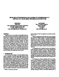
Figure 2.2: Schematic illustration of the model: as in Figure 2.1, green voxels contain single cells and red voxels contain two cells, giving rise to pressure sources. This pressure is propagated by a Laplacian operator over the voxels and induces a force, and hence a rate to move, for the cells in the subset of voxels indicated by the arrows. Cells in boundary voxels may move into empty voxels and cells in doubly populated voxels may move into voxels containing fewer cells. All arrows are drawn on a common scale. Here, D1 is the conversion factor from a unit pressure gradient into a movement rate to a voxel vj never visited before, D2 similarly, but into a voxel previously occupied, and D3 covers the “crowding” case where a cell in a doubly occupied voxel enters a singly occupied voxel. We generally assume D1 D2 , since the extracellular matrix contained in previously unvisited voxels is usually thought to be less penetrable than that of previously occupied voxels. To understand the scale of D3 we note that from the divergence theorem Z Z ~= − (∇p · n) dS s(u) dV. (2.14) ∂Ω
Ω
In other words, the total pressure gradient over any closed surface ∂Ω is equal to the enclosed sources. With ∂Ω the boundary surrounding the whole cell population, it follows that the ratio D2 /D3 expresses the preference for events at the tissue boundaries (cells entering empty voxels) to events internal to the region (cells in doubly occupied voxels moving to an already occupied neighbouring voxel). For example, assuming the presence of a single internal source voxel and that D2 /D3 ≡ 1, then the probability of a cell in the source voxel to move is the same as the total probability of a cell to move into any of the boundary voxels in ∂Ω. The rates (2.11)–(2.13) are illustrated on a common scale with D1 = D2 = D3 in Figure 2.2.
3
Results
We now present some computational results for the proposed modeling framework. In doing so we focus on highlighting the three distinct advantages of our approach: (1) the mechanics is based on constitutive equations obeying a well-understood physics; (2) the framework is fast and scalable, and therefore convenient to experiment with; and (3), it is also flexible and allows for a seamless coupling to other processes of interest. In §3.1 we look at the possible dependency of results on the underlying computational grid, and in §3.2 we investigate how to couple the cellular behaviour with signals in the local external environment. In §3.3 we couple the modeling framework with intracellular continuous-time processes, including cell-to-cell signalling and, finally, in §3.4 we demonstrate how the complex behaviours of a tumour model may be investigated. 8
3.1
Simulated cell population is free of grid artefacts
A disadvantage with grid-based methods and local update rules that has been highlighted in the literature is that grid artefacts may appear unless some care is exercised [38]. We test for grid artefacts by artificially forcing a number of cells into a square configuration and then relaxing the system to equilibrium (Figure 3.1). In the absence of any other mechanical forces, clearly, the equilibrium state should be approximately circular.
Figure 3.1: The set-up of the relaxation process experiment. Left: all voxels in a square initially contain two cells, middle and right: after relaxation the populated domain becomes approximately circular in shape where all voxels contain a single cell. In Figure 3.2 we quantify the average cellular density across N = 100 independent runs of the model and find that, although a very small memory effect from the initial data is still visible (left/right and up/down), there is no dependence on the underlying grid except for the natural distortions due to discreteness. This comes from the fact that the physics is based on well-understood constitutive equations and that we employ a grid-consistent discretization of the Laplacian (eqs. (2.4) and (2.8)).
Figure 3.2: Average concentration (N = 100 trials) after relaxation from square initial data. Left: Cartesian grid, right: hexagonal grid. The reference circle has the same area as the total cell population. Although a discrete effect is visible, there are no grid artefacts in the sense of preferred expansion directions.
9
3.2
Population-level behaviour via sensatory control
A notable extension of this basic framework is to model a population of cells that respond to external stimuli in their local environment. As our test case we take the two-dimensional migratory model of neurons responding to an inhibiting chemical known as Slit [6]. The cellular pressure, p, of the neurons is now described by the chemotaxis equation ∂p = ∇ · (∇p + pχ1 ∇S) + s(u), (3.1) ∂t where χ1 is the chemotactic sensitivity of the neurons to the chemical S, i.e., the concentration of Slit. The parameter εp is taken to be small and represents our assumption that the pressure equilibrates on a faster timescale than the movement of the neurons. The source term, s(u), is as defined previously. Eq. (3.1) represents the movement of cells down the gradients of the Slit concentration. We set the domain for the experiment to be ~x = (x1 , x2 ) ∈ R2 and the equation governing the concentration of Slit is given by εp
∂S = DS ∆S − kS + Qδ (x1 − L) , (3.2) ∂t where DS is the constant diffusivity of Slit, k is the rate of degradation and Q is the strength of the Slit source on the line x1 = L. The parameter εS is again taken to be small and represents the assumption that the diffusion of Slit occurs on a faster timescale than the movement of the cells. Imposing Assumption 2.2 thus allows us to solve the steady-state problem εS
where the boundary conditions for the Slit chemical are S(x1 , x2 ) → 0, ∂S → 0, ∂x1
as |x1 | → ∞,
(3.5)
as |x1 | → ∞.
(3.6)
We note that eqs. (3.4)–(3.6) can be solved analytically to give √ Q S(x1 , x2 ) = √ e− k/DS |x1 −L| . 2 kDS
(3.7)
We also include a pressure-independent movement mechanism, representing the active motion of the cells due to the chemo-repellent (see Assumption 2.1). To include the chemotaxis-driven movement of a cell from voxel i to voxel j we derive the following current Z eij I(i → j) = −χ2 (3.8) ∇S(~x) d~S = χ2 (Si − Sj ), dij vi ∩vj where χ2 is a measure of the affinity of the cells to Slit for this type of pressure-independent movement. We initialise a circular region, with radius r = 10, of doubly occupied sites in the centre of the domain, where the voxel size is taken to be h = 1. We specify the parameters [χ1 , χ2 , DS , k, Q, L] = [100, 5, 50, 0.1, 2, 50], and run 100 simulations until terminal time T = 1000. We present the average cell density profile in Figure 3.3. As expected, on average the cell population moves away from the source of Slit, consistent with it being a chemo-repellent. 10
50
x2
Figure 3.3: Average cell density (N = 100 trials) after relaxation from an initially circular explant (indicated by the black circle) with two cells in each voxel. The source of Slit is on the right-hand edge of the domain, at x1 = L, and we see that, on average, cells move preferentially to the left, away 50 from the source of Slit.
-50 -50
3.3
x1
Continuous-time mechanics allows for seamless coupling to cellular signalling processes
A great flexibility with the proposed framework comes from the fact that additional processes may be simulated concurrently with the overall mechanics of the cell population (see Algorithm 1, line 8). Notably, such processes may include cell-to-cell communication driving cell fate differentiation. To illustrate this we consider the classical Delta-Notch intracellular signalling model [7], which produces pattern formation via a simple lateral inhibition feedback loop. With (ni , di ), respectively, the Notch and Delta concentrations within cell i, this model takes the dimensionless form n0i = f (d¯i ) − ni , d0i = v (g(ni ) − di ) ,
(3.9)
where 0 denotes differentiation with respect to time and 1 X d¯i = dj , |Ni | j∈Ni
f (x) ≡
xk , a + xk
g(x) ≡
1 . 1 + bxh
(3.10)
We take parameters [a, b, v, k, h] = [0.01, 100, 1, 2, 2] and the average in eq. (3.10) is taken over the set of neighbours Ni of the cell i. Additional stochastic noise terms may also be added to (3.9), but for simplicity we let the model be fully deterministic. To produce a dynamic population we let the cells in the middle of the region proliferate at a constant rate and we terminate the simulation when Ncells = 1000. The average in eq. (3.10) is appropriately modified to account for any doubly occupied voxels. To get a more realistic contact pattern a hexagonal grid was used; hence each voxel has six neighbours. In Figure 3.4 a typical time-series of this model is summarised. Here the time-scale of the Delta-Notch dynamics, eq. (3.9), is on a par with that of the proliferation process, so that their dynamics equilibrates after the tissue stops growing. A second simulation is summarised in Figure 3.5, where the right-hand side of eq. (3.9) has been scaled by a factor of 50 so that the Delta-Notch model is in quasi-steady-state as the tissue grows.
11
Figure 3.4: Coupling cellular signalling in continuous time. Top left: initially cells are placed in a circular region (demarcated by the white circle) and all cells in this region are allowed to proliferate at a constant rate. Top right: the population thus grows and a Delta-Notch signalling model is simulated concurrently. Bottom left/right: the Delta-Notch model equilibrates after the cellular growth process has stopped. The times for these snapshots are t = [5, 40, 70, 100] units of time at unit proliferation rate, and the model was simulated using the Delta-Notch parameters described in the text.
Figure 3.5: Delta-Notch dynamics simulated anew, but on a faster time-scale. Here the process is essentially in continuous equilibrium as the tissue grows. These two frames correspond to the top right and bottom left frames of Figure 3.4.
12
3.4
Non-trivial dynamics emerges from the combination of grid-based physics and local behaviour
Finally, we utilise our proposed framework to build a model for avascular tumour growth. It is known that an important factor in the growth of tumours is the availability of oxygen to the tumour. In the case of an avascular tumour there is no direct supply of oxygen to the tumour itself, but instead oxygen in the surrounding tissue diffuses into the tumour. We consider the tumour to be a growing population of cells that can potentially proliferate and/or die over the course of the simulation. We extend the occupancy of voxels such that ui ∈ {−1, 0, 1, 2}, where ui = −1 corresponds to a dead cell occupying a voxel. The cells at the boundary of the tumour can consume oxygen and proliferate if the concentration of oxygen is sufficient. Further into the tumour, where the concentration of oxygen is generally lower, the cells continue to consume oxygen but can no longer proliferate; these are known as quiescent cells. Near the centre of the tumour the oxygen concentration is low enough that the cells die and eventually degrade; this region is known as the necrotic core. As before we solve the discrete Laplace equation (2.8) for the pressure in each voxel, with homogeneous Dirichlet boundary conditions (2.9) on the boundary ∂Ω, the collection of empty voxels that are adjacent to occupied voxels. We also have an equation for the oxygen concentration, c, which diffuses through the domain with sources at the fixed external boundary, ∂Ωext , thus, −Lc = −λa(u), ci = 1, i ∈ ∂Ωext ,
(3.11) (3.12)
where λ is the rate of consumption of oxygen for a single cell and a(ui ) is the number of alive cells (ui ∈ {0, 1, 2}) in the ith voxel (doubly occupied voxels consume twice as much oxygen and empty voxels or those containing dead cells consume no oxygen). From these discretised equations we can calculate all the different rates for the possible events. These events are as follows. A cell occupying its own voxel, ui = 1, will proliferate at rate ρprol if ci > κprol , where κprol is the minimum oxygen concentration for proliferation to occur. A living cell will die at a rate ρdeath if ci < κdeath , where κdeath is the threshold oxygen concentration for cell survival. In the case of cell death, ui = 1 is replaced with ui = −1. A dead cell, ui = −1, can degrade at a constant rate ρdeg to free up the voxel (ui = 0) for other cells to move in to it. We also include the rates for cell movement as shown in eqs. (2.11)–(2.13). In Figure 3.6 we present snapshots from a realisation of the model with parameters [D1 , D2 , D3 , λ, κprol , ρprol , κdeath , ρdeath , ρdeg ] = [0.01, 25, 0.01, 0.0015, 0.65, 0.125, 0.55, 0.125, 0.01] that demonstrates the evolution of the tumour into the classical regions of proliferating cells, quiescent cells and a necrotic core. The widely-held view in the field is that a limited oxygen supply leads to a stable, finite-sized tumour [25]. We sought to parameterise our model to replicate this behaviour. However, despite a thorough search of parameter space, we could not establish a finite-sized tumour; the best we could do was to significantly reduce the time-scale on which growth occurs by increasing the rate at which cells fill the space in the necrotic core due to cell degradation (by increasing D2 ). Furthermore, we found that after the tumour grew to a certain size the proliferating ring would break up and form asymmetric protrusions, thus increasing the surface area and consequently the oxygen available to the tumour.
13
Figure 3.6: Snapshots of a realisation of the avascular tumour model. Top left: initially cells are placed in an approximately circular region. Top right: cells have proliferated due to an initial abundance of oxygen. Bottom left: the generation of an oxygen concentration profile in the tumour drives the formation of three regions; the proliferative ring (red voxels); the quiescent region (green voxels); and the central necrotic core (black voxels). Bottom right: the tumour has grown asymmetrically with protrusions emerging on the tumour surface. The times for these snapshots are t = [0, 45, 270, 500] units of time, the model parameters are as given in the text.
4
Discussion
The goal of this work was to provide an efficient, hybrid and multiscale computational framework for modelling populations of cells at the tissue scale. Our approach draws upon a constitutive, mechanistic description of cellular biomechanics to drive expansion and/or retraction of the cell population as cells move and undergo proliferation and death. By assuming that the timescale on which the tissue relaxes to mechanical equilibrium is much shorter than that of other mechanical processes, we are able to assume that the “cellular pressure” within
14
the population is governed by the Laplace equation with specified boundary conditions and source terms. We then use the pressure gradient within the tissue to derive rate equations for the movement of cells within the population. This enables us to propagate the model in continuous time, using an event-driven algorithm such as that originally proposed by Gillespie [12]. A significant advantage of our approach in this regard is that both discrete and continuous models of biochemical signalling can easily and flexibly be incorporated into the framework. This enables the user to develop hybrid and multiscale models that include constitutive descriptions of cellular biomechanics, inter- and intra-cellular signalling in an efficient and scalable framework. We have demonstrated the utility of our approach using four examples. First, we demonstrated that, as expected, a simple colony of proliferating cells grows isotropically. Second, we demonstrated how to integrate signals from the local microenvironment into cell movement laws, using the migration of cells within a neuronal explant exposed to a gradient in the secreted protein Slit as an example. Our third example showed that it is easy to integrate cell-cell signalling models into the framework, using the delta-notch lateral inhibition model as a test case. Finally, we developed a model for avascular tumour growth, wherein cell proliferation and death is controlled by the local oxygen concentration, and the cell population generates an oxygen profile within the tumour as the cells consume oxygen. In summary, the real advance provided by our approach is the ability to quickly and efficiently simulate the behaviour of large populations of cells, in both two and three spatial dimensions. Our model is both hybrid and multiscale in nature; it can incorporate both continuum and discrete models of biochemical signalling both within and between cells. For the purpose of experimenting we have developed a serial Matlab implementation of the model that employs a direct factorisation of the discrete Laplace operator and, as such, scales conveniently to about 20,000 cells. Using a compiled language and parallelization one could likely improve upon this figure to some extent. However real savings in computing time will require optimal Laplace solvers that utilise, for example, algebraic or geometric multigrid techniques [28, 33] that can take advantage of the incremental nature of the computational process when the domain evolves slowly. We leave this aspect of the implementation for future work. In the modern era of biology, where quantitative data describing the evolution of cell populations and tissues can be collected with relative ease, we are now in a position to test and validate experimentally generated hypotheses using biologically realistic mechanistic models. However, these models need to be calibrated against the available data, and the sensitivity of model predictions to changes in model parameters needs to be explored. All of this requires repeated simulation of multiscale and hybrid cell-based models, the computational demands of which have to-date provided a barrier to significant progress. The DLCM method we outline here results in significant advances in our ability to efficiently simulate hybrid and multiscale cell-based models in two and three spatial dimensions, and therefore provides a very real opportunity to test and validate mechanistic models using quantitative data.
Acknowledgment REB would like to thank the Royal Society for Wolfson Research Merit Award. DBW would like to thank the UK’s Engineering and Physical Sciences Research Council (EPSRC) for funding through a studentship at the Systems Biology programme of The University of Oxford?s Doctoral Training Centre. 15
References [1] T. Alarcon, H. M. Byrne, and P. K. Maini. A cellular automaton model for tumour growth in inhomogeneous environment. J. Theor. Biol., 225:257–274, 2003. [2] A. R. Anderson and M. Chaplain. Continuous and discrete mathematical models of tumor-induced angiogenesis. Bull. Math. Biol., 60(5):857–899, 1998. [3] K. Atwell, Z. Qin, D. Gavaghan, H. Kugler, E. J. A. Hubbard, and J. M. Osborne. Mechano-logical model of C. elegans germ line suggests feedback on the cell cycle. Development, 142(22):3902, 2015. [4] B. Benazeraf, P. Francois, R. E. Baker, N. Denans, C. D. Little, and O. Pourqui´e. A random cell motility gradient downstream of FGF controls elongation of an amniote embryo. Nature, 466(7303):248–252, 2010. [5] G. W. Brodland and D. A. Clausi. Embryonic tissue morphogenesis modeled by FEMM. J. Biomech. Eng., 116(2):146–155, 1994. [6] A. Q. Cai, K. A. Landman, and B. D. Hughes. Modelling directional guidance and motility regulation in cell migration. Bull. Math. Biol., 68(1):25–52, 2006. [7] J. R. Collier, N. A. M. Monk, P. K. Maini, and J. H. Lewis. Pattern formation by lateral inhibition with feedback: a mathematical model of delta-notch intercellular signalling. J. Theor. Biol., 183:429–446, 1996. [8] F. R. Cooper, R. E. Baker, and A. G. Fletcher. Numerical analysis of the immersed boundary method for cell-based simulation. bioRxiv, 2016. [9] D. Drasdo and S. H¨ ohme. A single-cell-based model of tumor growth in vitro: monolayers and spheroids. Phys. Biol., 2(3):133, 2005. [10] R. Farhadifar, J.-C. R¨ oper, B. Aigouy, S. Eaton, and F. J¨ ulicher. The influence of cell mechanics, cell-cell interactions, and proliferation on epithelial packing. Curr. Biol., 17 (24):2095–2104, 2007. [11] A. G. Fletcher, M. Osterfield, R. E. Baker, and S. Y. Shvartsman. Vertex models of epithelial morphogenesis. Biophys. J., 106(11):2291–2304, 2014. [12] D. T. Gillespie. A general method for numerically simulating the stochastic time evolution of coupled chemical reactions. J. Comput. Phys., 22(4):403–434, 1976. [13] F. Graner and J. A. Glazier. Simulation of biological cell sorting using a two-dimensional extended Potts model. Phys. Rev. Lett., 69(13), 1992. [14] S. D. Hester, J. M. Belmonte, J. S. Gens, S. G. Clendenon, and J. A. Glazier. A multicell, multi-scale model of vertebrate segmentation and somite formation. PLoS Comput. Biol., 7(10), 2011. [15] J. Kursawe, R. E. Baker, and A. G. Fletcher. Impact of implementation choices on quantitative predictions of cell-based computational models. J. Comput. Phys., To appear., 2017. 16
[16] Y. Mao, A. L. Tournier, P. A. Bates, J. E. Gale, N. Tapon, and B. J. Thompson. Planar polarization of the atypical myosin Dachs orients cell divisions in Drosophila. Genes Dev., 25(2):131–136, 2011. [17] F. A. Meineke, C. S. Potten, and M. Loeffler. Cell migration and organization in the intestinal crypt using a lattice-free model. Cell Prolif., 34(4):253–266, 2001. [18] B. Monier, A. Pelissier-Monier, A. H. Brand, and B. Sanson. An actomyosin-based barrier inhibits cell mixing at compartmental boundaries in Drosophila embryos. Nat. Cell Biol., 12(1):60–65, 2010. [19] L. Naumov, A. Hoekstra, and P. Sloot. Cellular automata models of tumour natural shrinkage. Physica A, 390(12):2283–2290, 2011. [20] T. J. Newman. Modeling multicellular structures using the subcellular element model. In Single-Cell-Based Models in Biology and Medicine, pages 221–239. Springer, 2007. [21] H. G. Othmer and A. Stevens. Aggregation, blowup, and collapse: The ABC’s of taxis in reinforced random walks. SIAM J. Appl. Math., 57(4):1044–1081, 1997. [22] H. G. Othmer, S. R. Dunbar, and W. Alt. Models of dispersal in biological systems. J. Math. Biol., 26(3):263–298, 1988. [23] K. A. Rejniak. An immersed boundary framework for modelling the growth of individual cells: An application to the early tumour development. J. Theor. Biol., 247(1):186–204, 2007. [24] M. Robertson-Tessi, R. J. Gillies, R. A. Gatenby, and A. R. Anderson. Impact of metabolic heterogeneity on tumor growth, invasion, and treatment outcomes. Cancer Res., 75(8):1567–1579, 2015. [25] T. Roose, S. J. Chapman, and P. K. Maini. Mathematical models of avascular tumor growth. SIAM Review, 49(2):179–208, 2007. [26] M. Scianna and L. Preziosi. Hybrid cellular Potts model for solid tumor growth. In A. d’Onofrio, P. Cerrai, and A. Gandolfi, editors, New Challenges for Cancer Systems Biomedicine, pages 205–224. Springer Milan, Milano, 2012. [27] Y. Setty, D. Dalf´ o, D. Z. Korta, E. J. A. Hubbard, and H. Kugler. A model of stem cell population dynamics: in silico analysis and in vivo validation. Development, 139(1): 47–56, 2012. [28] K. St¨ uben. A review of algebraic multigrid. J. Comput. Appl. Math., 128(1–2):281–309, 2001. Numerical Analysis 2000. Vol. VII: Partial Differential Equations. [29] A. Szab´ o and R. M. H. Merks. Cellular Potts modeling of tumor growth, tumor invasion, and tumor evolution. Frontiers Onc., 3:87, 2013. [30] S. Tanaka. Simulation frameworks for morphogenetic problems. Computation, 3(2):197, 2015. [31] R. N. Thompson, C. A. Yates, and R. E. Baker. Modelling cell migration and adhesion during development. Bull. Math. Biol., 74(12):2793–2809, 2012. 17
[32] G. Trichas, A. M. Smith, N. White, V. Wilkins, T. Watanabe, A. Moore, B. Joyce, J. Sugnaseelan, T. A. Rodriguez, D. Kay, R. E. Baker, P. K. Maini, and S. Srinivas. Multi-cellular rosettes in the mouse visceral endoderm facilitate the ordered migration of anterior visceral endoderm cells. PLoS Biol., 10(2), 2012. [33] U. Trotter, C. W. Oosterlee, and A. Sh¨ uller. Multigrid. Academic Press, 2001. [34] B. Vasiev, A. Balter, M. Chaplain, J. A. Glazier, and C. J. Weijer. Modeling gastrulation in the chick embryo: Formation of the primitive streak. PLoS ONE, 5(5):e10571, 2010. [35] F. J. Vermolen and A. Gefen. A semi-stochastic cell-based model for in vitro infected ‘wound’ healing through motility reduction: A simulation study. J. Theor. Biol., 318: 68–80, 2013. [36] D. Walker, G. Hill, S. Wood, R. Smallwood, and J. Southgate. Agent-based computational modeling of wounded epithelial cell monolayers. IEEE Trans. Nanobiosci., 3(3): 153–163, 2004. [37] M. Weliky and G. Oster. The mechanical basis of cell rearrangement. i. Epithelial morphogenesis during Fundulus epiboly. Development, 109(2):373–386, 1990. [38] C. A. Yates and R. E. Baker. Isotropic model for cluster growth on a regular lattice. Phys. Rev. E, 88(2):023304, 2013. [39] C. A. Yates, R. E. Baker, R. Erban, and P. K. Maini. Refining self-propelled models for collective behaviour. Canadian Appl. Math. Q., 18(3):299–350, 2010. [40] Y. Zhang, G. L. Thomas, M. Swat, A. Shirinifard, and J. A. Glazier. Computer simulations of cell sorting due to differential adhesion. PLoS ONE, 6(10), 2011. [41] C. Ziraldo, Q. Mi, G. An, and Y. Vodovotz. Computational modeling of inflammation and wound healing. Adv. Wound Care, 2(9):527–537, 2013.