Modeling with uncertainty in continuous dynamical

Modeling with uncertainty in continuous dynamical systems: the probability and possibility approach

Gianluca Bontempi

IRIDIA, Université libre de Bruxelles, Brussels, Belgium e-mail: [email protected]

Modeling with uncertainty in continuous dynamical systems: the probability and possibility approach Gianluca Bontempi, Student Member, IEEE IRIDIA, Université libre de Bruxelles, Brussels, Belgium e-mail: [email protected]

Abstract This paper presents probability and possibility as two measures to model different types of uncertainty in continuous dynamical systems. We analyze and compare how probability and possibility distribution evolve in a dynamical system modeled by differential equations, where initial conditions and/or parameter may be uncertain. Moreover, we propose a new algorithm for the numerical resolution of a fuzzy differential system and we relate it to existing computational methods to solve regular stochastic differential equations. Finally, we compare results obtained by simulating a dynamical system in which uncertainty is first represented in a possibilistic and then in a probabilistic form.

1. Introduction This paper compares possibility and probability as two formalisms to represent different kinds of uncertainty in a continuous dynamical system. The notion of continuous dynamical system is a basic concept in system theory: it is the formalization of a natural phenomenon in a set of real variables, defined as the state, and a set of deterministic differential equations, defined as the model. The resolution of the system of differential equations provides the time evolution of the state variables, defined as the behavior of the system. The differential model of a dynamical system contains elements and operators that constitute a formal description of features of the phenomenon under examination. However, due to errors in the measurements, lack of precise knowledge or inherent randomness in the process, these elements may not be uniquely defined. The idea that there can be a lack of determinism in a deterministic set of equations appears at first to be a contradiction in terms. What enters here is the important distinction between mathematical precision and imprecise observations. The determinism we speak about in dynamical models is the property of the mathematical uniqueness of the solution, namely, given a precise initial condition of the system, there is precisely one evolution of the system satisfying both the equations of the model and the initial conditions. However, this mathematical determinism does not guarantee a

1

completely certain evolution, because it is not always possible to define initial condition and parameters of the model with an infinite accuracy. Uncertainty modeling within system theory and artificial intelligence has long been recognized as a topic worthy of investigation. In system theory uncertainty is classically treated in probabilistic form by the theory of stochastic processes. Research in artificial intelligence has enriched the spectrum of available techniques to deal with uncertainty by proposing new non probabilistic formalisms, as the theory of possibility (based on the theory of fuzzy sets) and the theory of evidence (Shafer, 1976). There has been a long debate on the relationships between probability and possibility as ways to model uncertainty (Bezdek, 1994). We suppose that in the context of dynamical systems, uncertainty stems mainly from two sources: low accuracy of measurement process and imprecise human knowledge (Smets, 1993). In the first case uncertainty originates from variability of data and weakness of sensors. Numerical quantitative measurements about initial condition and/or parameters may be available but they cannot define with certainty the model of the system. For example, consider a parameter representing the frequency of an event, as the number of faults per month in an industrial machine: this variable may be not known precisely but, if we have done a series of measurements of its value in the past, we may model its uncertainty with a probabilistic distribution. In the second case, uncertainty does not originate from unpredictable numerical measurements but from imprecise human knowledge about the dynamical system: as a consequence, only imprecise estimates of values and relations between variables may be available. Let us consider, for example, a variable representing the amount of heat dissipated in a steam generator in normal working conditions: it may be not convenient, for safety and/or cost reasons, to measure this quantity but a technical expert may qualitatively suggest its possible value (e.g. "about 90 KJoule"). In this situation, we consider a possibilistic distribution as a proper representation of the uncertain knowledge. This paper focuses on dynamical systems where initial conditions and/or parameters are described by uncertainty distributions. The main contribution of this paper is to present and compare the laws describing the time evolution of the probability and possibility distributions in a dynamical system. Moreover, we propose a new method to compute how possibilistic uncertainty, represented by fuzzy numbers, evolves in differential equations. This method is then compared with the Monte Carlo method, a well known computational method for stochastic systems.

2

The organization of this paper is as follows. We first review some fundamentals of dynamical systems and introduce probability measures and possibility measures as special types of fuzzy measures (Sugeno, 1977). Next, we recall how a probabilistic distribution evolves in a regular stochastic differential equation. Then, we present possibilistic differential equations in the context of the theory of fuzzy sets and numbers (Zadeh, 1965). The proposed method of numerical resolution is an extension of the method proposed in (Bonarini, Bontempi, 1994): we show how the problem of propagating a fuzzy distribution may be reduced to a problem of optimization, and we present our fuzzy algorithm of integration. Also, we make an analytical and computational comparison between probabilistic and possibilistic methods in dynamical systems. Finally, we compare results obtained by simulating a dynamical system in which uncertainty is first represented in a possibilistic and then in a probabilistic form.

2. Dynamical systems and ordinary differential equations (ODE) Consider a dynamical system whose state is composed of n scalar variables y i. Let its model be a system of n first order ordinary differential equations where the i-th component is the following dy i = Fi ( y, t; c) i = (1, dt

L , n)

c = (c1 ,

L, c ) k

(1)

Let the initial condition be y(0)=y0 with y0∈Rn, c a vector of control parameters and t the variable denoting time. c will be understood to be independent of t. (1) may be written in the corresponding abbreviated form •

y = F( y, t ; c)

y ∈ Rn , c ∈ Rk

(2)

We say that such a dynamical system has n as its dynamical dimension. We denote by y(t,y0) ≡ ( y1(t,y0), ...,yn(t,y0)) the solution of the system of differential equations (1)1. It is also understood that no yi(t)≡t . It is very useful to view (1) as describing the motion of a point y(t) in a ndimensional space, which will be called the phase space of the system. In fig. 1 we show the phase space of a 3-th order dynamical system, where a system trajectory starts in point y(0) at time t=0 and reaches point y(t*) at time t*.

1We remark that the solution y(t,y ) is a function of time and the initial condition: if we assume that 0

the inital condition is fixed, we denote the solution with y(t).

3

y3

y(t*)

Trajectory

y(0)

y2

y1

fig. 1 A trajectory in the phase space of a 3rd order dynamical system

We may easily reformulate the system (1) by eliminating the control parameters and adding for each of them a state variable whose evolution is governed by the following differential equation •

.

•

yn+ j = c j = 0

j = (1,..., k)

(3)

The system (1) now has the form •

y = F( y, t )

y ∈ Rn

(4)

If the functions Fi do not depend explicitly on time, the system is said to be autonomous, otherwise it is non autonomous. In a non autonomous system, more than one solution, say y(1)(t), y(2)(t) can pass through the same point of the phase space (i.e. y(1)(t*)= y(2)(t*) for some t*) (Jackson, 1991). To ensure that only one solution passes through each point, we will consider only autonomous systems •

y = F( y)

y ∈ Rn

(5)

The general solution of this equation is of the form y(t)=y(t,y0)

(6)

where y(0)=y(0, y0)= y0 is the prescribed initial condition. Equation (6) can be viewed as a continuous mapping in the phase space Yt:Rn→Rn, which carries the initial point y0 to the point y(t). If the dynamical solution exists and is unique, then to any given y(t) and t there must correspond a unique initial point y0, that is one can write y0=K(y(t),t). This is the inverse mapping of (6) and since the mapping is one-to-one and continuous, it is referred to as a homeomorphism (and if it is differentiable in t and in y0, a diffeomorphism) (Arnol'd, 1992).

4

2.1. Numerical solution of ordinary differential equations The problem of finding a solution to (5), satisfying a known initial condition y0, is called initial value problem. The solution y(t,y0) may be expressed in analytical or numerical form: in the first case y(t,y0) has an analytical expression, while in the second case numerical methods are employed to compute the values y(t*,y0) at desired instants t*. To obtain an exact analytical solution is possible only in the simplest cases. Indeed, several numerical methods have been developed to solve ordinary differential equations numerically. Runge-Kutta algorithms are the most popular, with predictor corrector and Burlish-Stoer algorithms being used where high accuracy is required, or where the equations are 'stiff' and not susceptible to relatively simple Runge-Kutta solution (Press et al., 1986).

3. Fuzzy measures of uncertainty So far, we have considered continuous dynamical system where all parameters and initial conditions are known in a precise way. We now introduce some measures that allow us to represent uncertainty in a deterministic dynamical system. Sugeno (1977) provided a general framework to the uncertainty measures by introducing the notion of fuzzy measure. A fuzzy measure g on a continuous set Y is a function g: 2Y→ [ 0 , 1 ] which assigns to each subset of Y a number in the unit interval [ 0 , 1 ]. In order to qualify g as a fuzzy measure, the function g must satisfy certain properties (axioms of fuzzy measures (Klir, Folger, 1988)). Two special types of fuzzy measures are the well-known probability measures and possibility measures. Let P : 2Y→ [ 0 , 1 ] be a probability measure P. By definition P ( A) = ∫ p( y )dy

(7)

A

is the probability measure of A for all A ∈ 2Y. The function p : Y → R+ is the probability density function and it satisfies the property ∫ p(y)dy = 1. Y Y Let us now denote a possibility measure by Π : 2 → [ 0 , 1 ]. We define Π(A)= max π (y)

(8)

y ∈A

5

as the possibility measure of A for all A ∈ 2Y where π : Y → [ 0 , 1 ] is the possibility distribution function. Definitions (7) and (8) reveal a substantial difference between the notion of probability and possibility: while the probability satisfies the property of additivity, this is not true for the possibility measure. Then, given two sets A, B ∈ 2Y with A∩B=∅ - P(A∪B)= P(A)+ P(B) while - Π(A∪B)= max(Π(A), Π(B)). As we show in the rest of the paper, the above properties characterize the behavior of probability and possibility in a dynamical system, .

4. Stochastic differential equations ( SDE ) The introduction of random elements into an ODE leads to the definition of stochastic differential equations. However, we should make precise what we intend for a stochastic differential equation since it depends on what we mean by derivatives of a stochastic process. A crucial point is the regularity (Sobczyk, 1990) of random functions occurring in the differential equation. If a very irregular random process occurs (as white noise processes) we have the so-called Ito stochastic differential equations. In these equations the uncertainty of variables and/or parameters is represented by adding to their deterministic value the effect of a random process of the white noise type. Consider a time varying parameter U(t) subject to some random effects: according to the Ito approach its uncertainty is modeled by U(t)=D(t)+"noise" where the probability distribution of the noise term is known and D(t) is assumed to be non random. When the random processes occurring in a differential equation are sufficiently regular the equations are called regular stochastic differential equations. In this case an uncertain constant parameter U is represented by a random variable with a known probability distribution. The theory of the Ito stochastic differential equations differs significantly from the theory of regular stochastic equations (Gardiner, 1985). In this paper we only examine the regular case. In fact, we introduce uncertainty in an autonomous dynamical system to model the incomplete knowledge about constant parameters and/or initial conditions: otherwise, the introduction of generalized random processes of the white noise type into the Ito SDE is adopted mainly to model dynamical systems subjected to rapidly time-varying random excitation. Let us now consider the regular differential equation •

y = F( y)

y ∈ R n y(0) = y 0

(9)

6

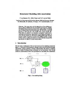
where y0 is a known random variable. The solution y(t,y0) of the stochastic initial value problem is still a regular stochastic process, which is completely characterized by its probability density p(y(t,y0)). 4.1. Regular SDE and the Liouville equation A well-known way to solve a regular stochastic initial-value problem is associated with the Liouville equation (Sobczyk, 1990 and Gardiner, 1985). Let us first introduce the concept of integral invariant. Let Ω(t) represent an arbitrary volume at time t in the phase space of (9), and let Ω(t+dt) represent the same volume at time t+dt (fig. 2); so Ω(t+dt) is the set of all points y(t,y0) that propagate according to (9) and such that y(t)=y0 is contained in Ω(t).

Ω (t+dt) y3

Ω (t) y 0

y2

y1 fig. 2 Evolution of a volume Ω(t) in the phase space of a 3rd order dynamical system

Let us consider the integral of some function f(y,t): Rn× R → R over this moving domain Ω(t), I(t) ≡ ∫

L ∫ f( y, t) dy ,L,dy 1

(10)

n

Ω(t)

f(y,t) is called an integral invariant of (9) if I(t) is constant in time. One basic result of stochastic theory is the Liouville theorem, which states that each function f(y,t) whose integral respect to the spatial variable is invariant during the evolution of the system, satisfies the following equation

7

[

]

∂ f( y, t) n ∂ + ∑ f( y, t)Fi ( y) = 0 ∂t i=1 ∂y i

(11)

which is commonly known as the Liouville equation. It has been demonstrated that the probability density p (y(t),t) is an integral invariant (Sobczyk, 1990), that is P(Ω(t)) = ∫ p( y, t)dy, is constant in time. Moreover, the Ω(t)

property of integral invariance implies that the Liouville equation (11) holds for the probability density: ∂ p( y, t) n ∂ p( y, t)Fi ( y) = 0 (12) + ∑ ∂t i=1 ∂y i

[

]

The Liouville equation is a first order partial differential equation and can be solved in general by the Lagrange method. It may be also transformed in the following ordinary differential equation holding along the trajectories of the system (Nicolis, Prigogine, 1977): dp( y, t) = − p( y, t) * divF( y) dt

(13)

where div is the divergence and is defined as ∂Fi i =1 ∂y i n

div F( y) = ∑

(14)

The probability density of a point in the phase space may be intuitively interpreted as the density of trajectories of the dynamical system at that point. When the divergence is null in the whole phase space, the dynamical system is conservative: this means that the volume of a region Ω(t), as the density of trajectories, remains constant during the evolution of the dynamical system (fig. 3.a). When the divergence is greater or smaller than zero, the system is said to be dissipative: if the divergence is greater than zero the system is divergent, the volume of a region Ω(t) increases and the density decreases (fig. 3.b). The opposite happens if the system is convergent.

8

y3

y3

y2

y2 y1

y1

dissipative divergent

conservative fig. 3a

fig. 3b

Then, the evolution of the probability measure in a dynamical system satisfies these two properties. Property 1. The probability density p(y(t,y0),t) along a trajectory y(t,y0) of a dynamical system is not constant (except for div F=0). Property 2. The probability of finding trajectories inside the time-variant volume Ω(t) is constant during the evolution of the dynamical system. It is worth remembering that the Liouville equation is a special case (the diffusion term is null) of the Fokker-Planck-Kolmogorov equation (Gardiner, 1985) that represents the evolution of probability distribution for the Ito stochastic differential equation. Therefore the regular SDE may be seen as a particular case of the more general Ito SDE. 4.2. Numerical solution of regular SDE By solution of a regular SDE (9) we mean a stochastic process satisfying the equation together with its probabilistic properties. Generally, as in the non random case, analytical solutions are not available. Most often, we can only obtain approximate solutions by numerical schemes. The Liouville equation can be used for the numerical computation of time evolution of the probability density. However, its major problem is that the numerical resolution of a partial differential equation implies a huge computational cost.. Another common resolution method is the MonteCarlo method (Korn, Korn, 1968). The Monte Carlo method is a statistical method for simulation that utilizes sequences of random numbers. It may be applied when the system is modeled by probability density functions. Thus, it is also used to simulate the evolution of a probability density in ordinary differential equations. Monte Carlo simulation of ODE is composed of the repetition of these three steps:

9

- a random sampling of the probability density of the initial condition distribution - a series of deterministic model simulations using as initial conditions the sampled values ("trials") - computation of the result by taking an average over the number of simulations. The set of simulated trajectories represents then a probabilistic sample of the solution of the stochastic differential equation.

We will now consider the properties of possibility measures, as an alternative formalism to represent uncertainty in a dynamical system. However, since the theory of possibility is based on the theory of Fuzzy Sets (Zadeh, 1965) (Dubois, Prade, 1980), we first review some fundamentals of this theory.

5. Fuzzy sets and fuzzy numbers Let Y be the universe set whose generic elements are denoted y. The membership of an element y to a subset A of Y can be represented by a characteristic function, or membership function (m.f.) µA: Y→{0,1} such that µA(y)=1 if y ∈ Α µA(y)=0 if y ∉ Α

(15)

When the valuation set {0,1} is extended to the real interval [0,1], A is called a fuzzy set. (16) Def. A fuzzy set A is normalized if ∃ y | µA(y)=1 Def. An α-cut of level h (0 ≤ h ≤ 1) of a fuzzy set A is the interval Ah={y∈ Α, µA(y) ≥ h }

(17)

Def. A fuzzy set A is convex iff its α-cuts are convex. Def. A fuzzy number is a convex, normalized fuzzy subset of the domain Y The concept of fuzzy number is an extension of the notion of real number: it encodes approximate but non probabilistic quantitative knowledge (Kaufmann, Gupta, 1985). For instance, let us consider a system (e.g. a steam generator) where it is not easy or convenient to measure a certain variable (e.g. its internal pressure); furthermore suppose that we have a qualitative, imprecise knowledge that in certain operating conditions the variable is around 5 bar. This does not imply a probabilistic distribution of the variable's value but rather a possibilistic distribution, which may be represented by a fuzzy number (fig.4).

10

m.f. 1.0

pressure

5

fig. 4 A fuzzy number

Zadeh has introduced both the concept of fuzzy set (Zadeh, 1965) and the concept of possibility measure (Zadeh, 1978). Zadeh's possibilistic principle (Zadeh, 1978) postulates µA(y)=πA(y) for all y∈Y

(18)

where µA(y) is the membership function of a fuzzy set A and πA(y) is the possibilistic measure of A. We rest on this principle to justify our use of fuzzy membership functions to represent possibilistic information. 5.1. Fuzzy functions A fuzzy function can be understood in several ways according to where fuzziness occurs (Dubois, Prade, 1980). We are considering deterministic models, then we will consider only ordinary functions that just carry the fuzziness of their arguments without generating extra fuzziness themselves. In such cases, we can apply the socalled fuzzy extension of non fuzzy functions by the extension principle introduced by Zadeh (1965). This principle provides a general method for extending standard mathematical concepts in order to deal with fuzzy quantities (Dubois, Prade, 1980). Let Φ:Y1× Y2×...×Yn→Z be a deterministic mapping from Y1× Y2×...×Yn to Z such that z=Φ(y1,y2,...,yn). The extension principle allows us to induce from n input −

−

fuzzy sets yi on Yi an output fuzzy set z on Z through Φ given by µ − (t) = z

sup

t = Φ(s1 ,s2 ,...,s n )

 min  µ − (s1 ), µ − (s2 ),  y1 y2

L, µ

 (s n )   y n1 −

(19)

or µ − (t) = 0 if Φ−1 (t) = ∅ z

−

where Φ − 1 (t) = 0 is the inverse image of t and µ − is the m.f. of y i (i=1,...n). yi

In the next section, we will use the extension principle to define fuzzy differential equations.

11

6. Fuzzy differential equations (FDE) Let us consider a fuzzy differential equation •

y = F( y) y ∈ R n y(0) = Y0

(20)

with Y0 fuzzy initial condition defined on the n-dimensional domain Y. We interpret this notation as a fuzzy extension of a non fuzzy differential equation. We consider a fuzzy differential equation as a deterministic differential equation where some coefficients or initial condition are uncertain and not representable in a probabilistic form: its solution is then the time evolution of a fuzzy region of uncertainty which corresponds to the possibility distribution in the phase space. The following theorems characterize some properties of this solution. Theorem 1. Let Y*=Y(t*,Y0) be the state of the fuzzy differential equation (20) at time t*. Then its value is given by µ Y* ( y*) = µ Y0 ( y 0 ) y* = y(t * , y 0 ) .

(21) •

where y=y(t,y0) is the solution of the non fuzzy system y = F( y) y ∈ R n y(0) = y 0 . Proof. The fuzzy value Y* of the state at time t* may be computed by the extension principle in this way sup µ Y* ( y*) =

y 0 ∈ Y0 : y*= y ( t * ,y 0 )

µ Y0 ( y 0 )

According to the solution of the initial value problem there is only one trajectory y(t,y0) passing through the point y* at time t*: it follows that µ Y* ( y*) = µ Y0 ( y 0 ) in which y*= = y(t*,y0).

+

Theorem 2. In a fuzzy differential equation the value of the probability distribution is constant along the trajectories of the system. Proof. According to the theorem 1, µ(y(t,y0))=µY0(y0) along a trajectory y(t,y0). Then, according to the Zadeh's possibilistic principle (18) π(y(t,y0))=µ(y(t,y0))=µY0(y0)= constant

+

Theorem 3 Let Ω(t) represent an arbitrary volume at time t in phase space of the fuzzy differential system (20) and Π(Ω(t)) be the possibility measure of this set. Then, Π(Ω(t)) is time invariant.

12

Proof. Given that the value of the possibility distribution π(y(t)) is time invariant along a trajectory y(t) for the theorem 2, and that Π(Ω(t)) = sup π ( y(t)) we may y (t)∈Ω(t)

deduce that also Π(Ω(t)) is time invariant.

+

To interpret intuitively these results let us consider a solution (trajectory) of the system passing through the point y1=y(t1,y0) at time t1 and through the point y2=y(t2,y0) at time t2. What the theorem 2 tells us is that the possibility that a trajectory passes through y1 at t1 is equal to the possibility that a trajectory passes through y2 at time t2. Moreover, if we consider a region Ω(t) that evolves according to the model of the system, for the theorem 3 the possibility of finding a trajectory in Ω(t1) at time t1 equals the possibility of finding a trajectory in Ω(t2) at time t2. 6.1. Numerical solution of a fuzzy differential equation The Extension Principle provides a method to compute the fuzzy value of a fuzzy mapping but, in practice, its application is not feasible because of the infinite number of computations it would require. Our approach considers instead fuzzy calculus as an extension of interval mathematics by the α-cut notion. A fuzzy computation may be decomposed into several interval computations, each one having as arguments the α-cut intervals of the fuzzy arguments at the same level. The results are the α-cuts of the fuzzy results (Nguyen, 1978). Then, the following relation holds for the mapping (19) z = ϕ ( y , y ,..., y ) = ϕ ( y , y ,..., y ) nh h 1 2 nh 1h 2h with z and y α-cuts of h-level of the fuzzy numbers z and yi, respectively. ih h Every fuzzy computation, even if differential, may be then decomposed into the repetition of more interval computations. From now on we will treat only interval computation. 6.1.1 Interval differential equations (IDE) Let us consider a system of interval differential equations (IDE) where the initial condition Y0α α is the α-cut of the fuzzy initial condition Y0 in the FDE (20). •

y = F( y) y ∈ R n y(0) = Y0α

(22)

This is the differential equation α-cut of the corresponding fuzzy differential equation (20). Let us define as solution Yα(t) of (22) the set of solutions of the ordinary differential equation whose initial condition belongs to Y0α α.

13

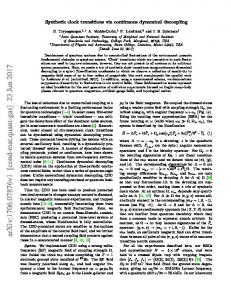
6.1.2 Numerical solution of IDE To solve numerically the system (22) it might seem intuitive to apply the interval mathematics (Moore, 1966) directly to the numerical algorithms introduced in Section 2.1. However, in (Bonarini, Bontempi, 1994) we have shown that a straightforward use of interval mathematics for the resolution of fuzzy (or interval) differential equation can produce incorrect results. This is due to the fact that the fuzzy (and interval) formalism is unable to represent the interaction that the differential equation establishes between variables: as a consequence, spurious values are introduced into the solution and the evolution of the system may reach region where no numerical solution exists. Figure 5 illustrates the problem. The figure plots the evolution of the initial condition (i.e. the rectangle ABCD) in a oscillatory 2-nd order system: if we represent the uncertain state of the dynamical system at time t' in the interval formalism, we introduce in the solution spurious points (black regions) which are not the evolution of points belonging to ABCD.

A

B

C

D

A' C' B' D'

fig. 5 Introduction of spurious trajectories in the non interacting simulation of an oscillating system

Our approach is instead the following: the initial condition of the interval differential equation defines an hyper cube. We call this n-cube the region of uncertainty of the system at time t=0. To solve the IDE means to compute the evolution in time of the region of uncertainty. We proved that under general conditions of continuity and differentiability it is sufficient to compute the evolution of the external surface of the uncertainty region (Bonarini, Bontempi, 1994). We demonstrated that

14

Theorem 4. An ordinary autonomous differential equation maps the external surface of its region of uncertainty at time t into the external surface of its region of uncertainty at time t+dt. The validity of the theorem leads to the conclusion that it is sufficient to calculate the trajectories of the points belonging to the external surface of the region of uncertainty to know the evolution in time of the region itself. However, the quantity of trajectories to be computed is still infinite, also if it is of a lower order. The problem remains how to sample, in the most convenient way, the external surface of the region of uncertainty during its time evolution. We extend the approach, presented in (Bonarini, Bontempi, 1994) by reducing this sampling problem to an optimization problem. To find the numerical solution of an IDE means to know at each time step t* the maximum and the minimum value of each state variable yi. These values are obtained by trying to maximize and minimize at time t* the functions yi(t*,y0). We may then use a constrained multivariable optimization algorithm to find the extremes of the functions yi(t*,y0) i=1...n where t* is fixed and the argument y0 is constrained to range over the external surface of the initial region of uncertainty. Let us remind that the performance of a multivariable optimization algorithm may be greatly increased by providing to it the partial derivatives (gradient) of the function value respect to the arguments: in our case we should provide the derivatives at time t * of yi respect to y0∈Y0α. To obtain these derivatives we use the connection matrix (Moore, 1966), as follows. We denote by y(t,y0) the n-dimensional, real vector solution to the numeric initialvalue problem. We define the connection matrix for the solution y(t,y0) as the matrix C(t,y0) with elements −

c ij =

∂yi ( t, y)

(23)

−

∂ yj

−

y= y0

We denote by J(t,y0) the Jacobian matrix of the vector function evaluated at y(t,y0). The matrix J(t,y0) has elements Jij (t, y0 ) =

∂Fi ( y) ∂y j y= y( t,y )

(24)

0

Moore (1966) demonstrated that ∂C(t, y 0 ) = J(t, y 0 ) ⋅ C(t, y 0 ) ∂t

(25)

15

with C(0,y0) = I where I is the identity matrix. The elements of the matrix give the sensitivity of the solution components yi(t,y0) with respect to small changes of the initial values (y0)i. By coupling the IDE system with the set of n2 equations coming from the connection matrix differential system we obtain an augmented differential system 2 which gives at time t* the values of the variables yi and the values of the derivatives of the variables yi respect to the initial condition y0. We may then use these combined values as the value and the gradient of the function to be maximized (or minimized), respectively. The central part of the algorithm is structured in the following steps: (i) the optimization routine takes a starting point y0 in the external surface of the initial uncertainty region; (ii) this point is passed to the routine of ODE numerical integration which uses y0 as initial condition and returns the value y(t*,y0) and the gradient values; (iii) if the optimization routine considers y(t*,y0) as a maximum (minimum) the algorithm stops; otherwise, the value y(t*,y0) and the gradient are used to sample a new point y0 and the execution returns to point (ii).

2Let us consider for example the Van Der Pol system

 . z = − (y ⋅ y − 1) ⋅ z − y  .  y=z

The augmented system, including the terms of connection matrix, with initial conditions is  z ( 0) = z 0  y ( 0) = y  0  . z ∂ z y y z y ( ) = − ⋅ − ⋅ − 1   ( 0) = 1 .  ∂z0  y = z  ∂z   ( 0) = 0 ∂y  ∂z ∂z   d ∂z d ∂z    0      dt ∂z 0 dt ∂y 0  −( y ⋅ y − 1) − (2 ⋅ y ) ⋅ z − 1 ∂z 0 ∂y0  ∂y (0) = 0   d y d y = ⋅  y y   ∂z0 ∂ ∂ ∂ ∂ 1 0        dt ∂z dt ∂y  ∂y  ∂z 0 ∂y0   0 0  ∂ y ( 0) = 1  0

16

Let us consider as example a second order IDE (fig. 6): the external surface at time t=0 is the square ABCD: it is transformed by the differential equation into the region A'B'C'D' at time t*. For each of the 4 parts (e.g., the segment AB) of the external surface of ABCD, the optimization algorithm searches the maximum and the minimum of the correspondent transformed part (e.g., the curve A'B'). The greatest of the maxima and the smallest of the minima are the extrema values of yi. y2

t=t*

y2_max(t*)

A'

B'

C' y2_min(t*)

D' B

A

y1 y1_min(t*)

y1_max(t*)

D

C

t=0

fig. 6 Evolution of the external surface of the region of uncertainty for a 2-nd order system

Let us remind, anyway, that we want a method of numerical resolution for a fuzzy differential equation. This procedure must be then repeated for each α-cut that decomposes the fuzzy initial value. The number of the α-cuts to be considered depends on the desired degree of accuracy. At this regard, it is important to remark that the region of uncertainty corresponding to an α-cut of level h1 is always contained into the region of uncertainty corresponding to an α-cut of level h2, if h1>h2 (Bonarini, Bontempi, 1994). Here it is the complete fuzzy algorithm in a pseudo programming language

17

for each α-cut for t*=initial_time to final_time for each variable yi yi_max(t*)=-Infinity yi_min(t*)=Infinity for each component Y0j of the external surface of the initial region of uncertainty j=1...2n yij_max(t*)= max(yi(t*,y0))  (y0 ∈ Y0j & yi(t*,y0) is a solution of (20)) yij_min(t*)= min(yi(t*,y0))  (y0 ∈ Y0j & yi(t*,y0) is a solution of (20)) yi_max(t*)=max(yi_max,yij_max) yi_min(t*)=min(yi_min,yij_min) end for end for end for end for table 1

This algorithm has been implemented in Matlab language (The Mathworks, 1992), by combining together the algorithms of optimization, resolution of differential equations and symbolic computation provided by this mathematical tool. The Symbolic Toolbox is used to automatically create the augmented differential system by computing the Jacobian of the original differential system. The Optimization Toolbox provides the algorithm of constrained optimization constr. The Matlab routine ode23 performs numerical integration. Moreover we used the graphical facilities of Matlab to present results of fuzzy simulation. 6.1.3 Remarks The proposed method goes one step further with respect to the non interacting algorithm proposed in (Bonarini, Bontempi, 1994): the heuristic criterion to choose the trajectories is now replaced by an optimization algorithm whose task is to choose the points to be simulated in order to reconstruct the region of uncertainty at a given t*. This does not guarantee to obtain the absolute maximum and minimum but the degree of performance is analogous to that of a gradient-based algorithm of optimization in front of a multivariable function. In terms of computational complexity it is necessary to remember two drawbacks of the present approach: (i) the complexity is an exponential function of the order n of

18

the dynamical system (2n is the number of components of the external surface of the initial region of uncertainty) (ii) the fuzzy solution at time t* is not computed by starting from the fuzzy solution at the previous instant (t*-dt): in fact, there is no guarantee that the trajectories considered to compute the extremes of the region of uncertainty at time (t*-dt) are the same trajectories to be considered at time t*. Then, at each time t* the trajectories must be computed starting from the time t=0. This implies an heavy computational charge when t* becomes high.

7. Probability vs. possibility in differential equations There exists a certain amount of literature debating the problem of the relation between possibility and probability (Bezdek, 94). In the sections 4 and 6 we have shown how probability density and possibility distribution evolve differently along the trajectories of a dynamic system: while probability changes according to the Liouville equation, possibility remains constant. We us now discuss the relation between these two formalisms in analytical and computational terms. 7.1 Probability vs. possibility in analytical terms Let y(t) be a point in the phase space of the dynamical system. The probability that the state belongs to a infinitesimal volume Ω(t) around y(t) is p(y(t),t)⋅Ω(t). Given the property of integral invariance p(y(t),t)⋅Ω(t) = p(y(t+dt),t+dt)⋅Ω(t+dt). Then along a trajectory, the quantity p(y(t),t)⋅Ω(t) remains constant. That is the following relation holds d ( p( y(t),t) ⋅ Ω(t) ) = 0 dt This implies •

(26)

•

p( y(t),t) ⋅ Ω(t) + p( y(t), t) ⋅ Ω(t) = 0 From the Liouville equation (13) we have •

− p( y(t), t) ⋅ div F( y(t)) ⋅ Ω(t) + p( y(t),t) ⋅ Ω(t) = 0 Then along the trajectories where p(y(t),t) is different from zero we have •

Ω(t) = Ω(t) ⋅ div F( y(t))

(27)

We may use the formula (27) to obtain • dπ ( y(t), t) d (π ( y(t), t) ⋅ Ω(t)) = ⋅ Ω(t) + π ( y(t), t) ⋅ Ω(t) dt dt = π ( y(t),t) ⋅ Ω(t) ⋅ div F( y(t))

19

(28)

Consequently, the evolutions in time of probability and possibility are summarized by the following equations dp( y(t),t) = − p( y(t), t) ⋅ div F( y(t)) dt d(p( y(t), t) ⋅ Ω(t)) =0 dt d(π ( y(t), t)) =0 dt d(π ( y(t), t) ⋅ Ω(t)) = π ( y(t),t) ⋅ div F( y(t)) dt

(29a) (29b) (29c)

(1)

(29d)

The first consideration we may deduce concerns what Zadeh called possibility/probability consistency principle. Zadeh (1978) defined a degree of consistency γ of the probability density p with the possibility distribution π. We extend Zadeh's definition to a continuous domain Y by γ (t) = ∫ π ( y(t), t) ⋅ p( y(t), t) ⋅ dy

(30)

Y

Let us notice that when γ is closer to 1, the consistency is higher. We may demonstrate the following theorem: Theorem 5. Consider a dynamic system where the uncertainty of the initial condition is represented both in probabilistic and in possibilistic form. If the initial probability density is consistent with the initial possibility distribution (γ=1) then this consistency is conserved during the system's evolution. Proof. γ =1 means that p(y)>0 implies π(y)=1. Then, from the differential laws of evolution (29a) and (29c), we can see that the consistency is conserved during the system evolution.

+

Our second consideration refers to the definition of a parameter relating possibility and probability density evolution along a system trajectory. Theorem 6. Let us define η(y(t),t) so that η(y(t),t)=

p( y( t), t) π ( y( t), t)

(31)

The time evolution of η is governed by the following differential law • p(y(0), 0) η (y(t),t)= -η(y(t),t)*div F (y(t),t) with η(0)= (32) π ( y(0), 0)

20

Proof. For the time invariance of π(y(t),t) (formula (29c)) and the formula (29a) we •

p( y(t),t) − p( y(t), t) ⋅ divF( y(t)) = = −η ( y(t),t) ⋅ divF( y(t)) have η (y(t),t)= π ( y(t), t) π ( y(t), t) . •

+

This differential relation permits to obtain a probability density value p(y(t),t) from the related possibility distribution π(y(t),t) and vice versa, once we know the initial p(y(0), 0) . We may then conclude that not only the consistency property distribution π ( y(0), 0) is satisfied but also that it is possible to define a parameter η relating probability and possibility, whose evolution depends on the model of the dynamical system. 7.2 Monte Carlo and FDE The different analytical properties between probability and possibility, studied in the previous section, suggest the adoption of specific methods to solve numerically SDEs and FDEs. However, Fishwick (1990) proposed the stochastic Monte Carlo method also for the numerical resolution of a fuzzy differential equation when the initial distribution is a normalized fuzzy distribution. We will now demonstrate that the Monte Carlo approach cannot be correctly used when we are dealing with possibility, even if its distribution is normalized. Let us consider the differential laws of evolution for probability (29b) and possibility and (29d). In the stochastic case, the homeomorphism between Ω(t) and Ω(t+dt) and (29b) implies that the probability of being at time t in Ω(t) equals the probability to be at time t+dt in Ω(t+dt). Then if we make a random sampling in Ω(t), the evolution of these points according to (9) determines a random sampling in Ω(t+dt). As a consequence, a random sampling of the initial condition produces a consistent random sampling of the stochastic solution. This property justifies the adoption of a Monte Carlo method in the probabilistic setting. If instead we want to interpret the initial normalized distribution as a possibility distribution, the law (29d) states that a random sampling on the initial condition does no more imply a random sampling on the possibilistic solution. In a dynamical system, generally, the quantity π(t,y(t))dΩ(t) is not time invariant. Therefore, the use of the Monte Carlo approach to evaluate the evolution of a normalized fuzzy distribution in a deterministic system is not justified. 7.3 Probabilistic vs. possibilistic computational methods The type of uncertainty affecting the model determines what method of simulation use. While the Monte Carlo method appears the most effective in the simulation of a

21

regular SDE, our algorithm (table 1) seems well suited to simulate a fuzzy differential equation. Even if they cover different situations, it may be interesting to compare the two methods in terms of computational complexity and reliability. Monte Carlo is simply the repetition of previously fixed number of numerical simulations. This means better performance in terms of complexity (see par. 6.1.3) with respect to the fuzzy method, but worse reliability. In fact, for a general differential equation there is no indication about the number of random trajectories to be considered. A random sampling on the initial condition transforms itself into a consistent random sampling but we cannot be sure that the number of samples which characterizes with a certain approximation the initial probability distribution are still significant with the same tolerance during the system evolution. Let us consider for example a divergent system whose initial probability distribution is normal with mean µ. Let us take n random samples from this distribution and assume that m and S represent the sample mean and the variance, respectively. The S confidence interval for µ is3 m±tα ( ) (Weiss, 1993): this means that the 2 n m− µ P( − tα ≤ ≤ tα ) that the real value of µ is inside the interval probability S 2 2 n S ) is 1-α. If we consider a successive time instant, the variance S of the m±tα ( 2 n sample increases and the confidence in the value of m, as estimate of µ, decreases (i.e. we have a greater interval of confidence). Then, in this case a fixed number of samples determines a continuous deterioration of the estimate. In our fuzzy approach, on the contrary, we use a gradient based optimization algorithm at each time step to determine how many trajectories are necessary to describe the possibility distribution. The number of trajectories does not only depend on the initial distribution of possibility but also on the model's structure.

8. Experiments We present two simulations of a dynamical system, model of a real mechanism, in which uncertainty is first represented in a possibilistic and then in a probabilistic form. Let us consider the physical system in fig. 7 (Borrie, 1992): a rod of mass M and moment of inertia I, which is rotable at one end round a horizontal axis and driven

3 t is the Student t-distribution. tα denotes the t-value with area α to its right under a t-curve (Weiss,

93)

22

by a motor gearbox that supplies a torque u. The whole arrangement is mounted on a table subject to vertical displacement whose unknown acceleration is w.

rod

motor

θ

table w

fig. 7 Experimental non linear device

The angular behavior of the rod is modeled by the following (heuristic) non linear equation, derived using Lagrangian mechanics: ..

.

I θ + f θ + Mgl cosθ = u − Ml cosθ w where θ is the angular position of the rod, f is the frictional torque, l is the distance from the axis to the center of gravity . Let us model the uncertain acceleration in the possibilistic case by the uniform fuzzy set described in fig. 8, and in the probabilistic case by an uniform probability distribution between 0.0 and 1.0. Let us simulate the system by our fuzzy resolution method and by Monte Carlo. In fig. 9 we have the evolution of the possibility distribution of θ in time: we have plotted the α-cut corresponding to the base (in this case a single α-cut describes the whole fuzzy number). In fig. 10 we have the evolution of the 100 random trajectories of θ obtained by sampling its initial probability density . m.f. 1.0

0.0

0.5

1.0

w

fig. 8 Fuzzy uniform distribution of the vertical acceleration

23

−0.7

−0.8

−0.9

−1

−1.1

−1.2

−1.3

−1.4 0

5

10

15

20

25

30

fig. 9 Possibilistic system evolution according our fuzzy algorithm

24

35

40

45

−0.7

−0.8

−0.9

−1

−1.1

−1.2

−1.3

−1.4 0

5

10

15

20

25

30

fig. 10 Probabilistic system evolution according Monte Carlo method

Analyzing the random Monte Carlo evolution it is possible to have an indication of the evolution of the probability density but as stressed before we must suppose that the number of samples is sufficient for that.

9. Conclusion In this paper we have presented and compared probability and possibility as two formalisms to represent and propagate uncertainty in a continuous dynamical system. Probability and possibility can be used as fuzzy measures on the dynamical phase space to describe two different kinds of uncertainty: the uncertainty that originates from random measurements, and the uncertainty that stems from imprecise human knowledge. Starting from the basic properties of system theory and fuzzy measures, we have showed that different, but related, analytical laws describe the behavior of probability and possibility in dynamical systems. We have made this relation precise

25

35

by the introduction of a parameter, whose evolution is characterized by a differential equation derived by the system model. The different analytical properties suggest the adoption of specific computational methods to simulate the evolution of possibilistic and probabilistic dynamical systems. While Monte Carlo methods are traditionally used when the uncertainty is represented in probabilistic form, we have proposed a simulation algorithm for systems where the initial conditions and/or parameters are represented by possibilistic distributions. Unlike the Monte Carlo method, our method may adapt the number of trajectories considered to the changing complexity of system dynamics. Some fields of engineering are interested in a non stochastic representation of uncertainty in dynamical systems, like Fuzzy Control and Identification. We believe that a comparative analysis with related stochastic methods may be useful to better understand the differences and the relative merits of both these approaches. We hope that the study proposed in this paper, may help in this analysis.

Bibliography [1] A RNOL 'D C OOK , Ordinary differential equations, Springer-Vaerlag, Berlin (1992). [2] BEZDEK J.C Editorial: Fuzziness vs. Probability - Again (!?). I E E E Transactions on Fuzzy systems,2,1,(1994), 1-3. [3] BONARINI A. AND BONTEMPI G. A qualitative simulation approach for fuzzy dynamical models. ACM Transactions on Modeling and Computer Simulation (TOMACS), 4, 4, (1994). [4] B ORRIE J.A. Stochastic systems for engineers, Prentice Hall, New York, (1992). [5] DUBOIS D. AND PRADE H. Fuzzy Sets and Systems, Academic Press, New York (1980). [6] F ISHWICK P.A. Fuzzy Simulation: Specifying and Identifying Qualitative Models. International Journal of General Systems, 19, (1990), 295-316. [7] G ARDINER C.W. Handbook of stochastic methods, Springer-Verlag, Berlin (1985). [8] JACKSON E.A. Perspective of nonlinear dynamics, Cambridge University Press, (1991). [9] K AUFMANN A. AND G UPTA M. Introduction to fuzzy arithmetic: theory and applications, Van Nostran d Rehinold, New York, NY, (1985). [10] KLIR G.J AND FOLGER T.A. Fuzzy sets, uncertainty, and information, PrenticeHall, New York (1988).

26

[11] K ORN G.A. AND K ORN T.M. Mathematical handbook for scientists and engineers, McGraw-Hill (1968) [12] THE MATHWORKS INC. MATLAB Reference Guide, Version 4.0 (1992) [13] MOORE R.E. Interval Analysis, Prenctice-Hall, Englewood Cliffs, NJ, (1966). [14] NICOLIS G., PRIGOGINE I. Self Organisation in Nonequilibrium Systems,Wiley, New York, (1977). [15] N GUYEN H.T. A note on the Extension Principle for Fuzzy Sets. Journal of Mathematical Analysis Applications, 64, 2, (1978), 369-380. [16] P RESS W. H., FLANNERY B., TEUKOLSKY S.A. AND V ETTERLING W.T. Numerical Recipes: the art of scientific computing, CUP, Cambridge, (1986). [17] S HAFER G. A mathematical theory of evidence, Princeton University Press, Princeton, NJ, (1976) [18] SMETS P. Imperfect information: imprecision, uncertainty. Technical Report: TRIRIDIA-93-3, Université Libre de Bruxelles ULB (1993). [19] SOBCZYK K. Stochastic Differential Equations with applications to physics and engineering, Kluwer Academic Publishers, Dordrecht, (1990). [20] SUGENO M. Fuzzy measures and fuzzy integrals: a survey. M.M. Gupta, G.N. Saridis and B.R. Gaines, eds., Fuzzy Automata and Decision Processes. North Holland, Amsterdam, 89-102, (1977). [21] WEISS N. A. Elementary statistics (2nd ed.) Addison Wesley (1993) [22] ZAHED L.A. Fuzzy Sets. Information and Control, 8, (1965), 338-353. [23] Z ADEH L.A. Fuzzy sets as a basis for a theory of possibility. Fuzzy Sets and Systems, 1, 1, (1978), 3-28.

27