For example, MOSAIK [5] performs complete se- quence alignment to find insertion/deletion differences us- ing Sanger and newer sequencing technology reads.
Scalable Modular Genome Assembly on Campus Grids Christopher Moretti, Michael Olson, Scott Emrich, and Douglas Thain Department of Computer Science and Engineering University of Notre Dame prove the quality of the assembly generated. Because of the complexity of this application, parallelization of some kind is required. The overlap step is the most naturally parallel, requiring millions of pairs of sequences to be compared to each other using a self-contained alignment algorithm. No task requires inter-computation communication or has dependencies on prior tasks. Most previous approaches to parallelizing assembly have focused on programming models and hardware architectures for tightly-coupled parallelism, requiring dedicated high performance clusters or massively parallel supercomputers. But, given the nature of the computation, it should be possible to perform assemblies on commodity hardware that is more flexible, affordable, and plentiful. As universities continue to form their own genome centers armed with “next-generation” DNA sequencers, more and more domain experts will need to perform assemblies, but few will have dedicated access to high end clusters and supercomputers. Instead, we may harness the large amounts of commodity hardware available in large campus computing grids that consist of hundreds or thousands of conventional desktop machines. Of course, this environment is not trivial to harness: variations in performance, network topology, and reliability make a campus grid an unforgiving programming environment. Ideally, users should be shielded from these difficulties, and simply be allowed to scale up existing sequential codes. To address this need, we present a framework for harnessing large scale campus grids for large scale genome assemblies. We present a modular framework that allows the end user to plug in any custom sequential alignment function, without requiring any special knowledge of parallel programming. The alignment function may be written in any language or environment familiar to the user. The framework accepts responsibility for dealing with failures and performance variations, and requires no shared file system. We show results of this framework for several assembly problems ranging from 100 thousand to 8 million sequences using campus grid resources ranging from a small cluster to several hundred nodes at each of three institutions. These
Abstract Bioinformatics researchers need efficient means to process large collections of sequence data. One application of interest, genome assembly, is naturally parallel; however, most current implementations are tied to uncommon high end hardware. We solve this problem by introducing a modular, scalable framework for genome assembly that runs on a wide variety of distributed environments without forcing end users to purchase specialized hardware or become experts in parallel programming. For large problems, the framework carefully handles task and data management while also achieving fault-tolerant speedup with good efficiency on several scales of resources. We show results for several assembly-related problems ranging from 738 thousand to over 84 million alignments using campus grid resources ranging from a small cluster to several hundred nodes at each of three institutions. These results show strong scaling beyond 512 nodes using a custom alignment module.
1 Introduction Even using state-of-the-art methods, the process of genome sequencing yields DNA sequences whose lengths vary from 25 to 1000 bases, depending on the technology used. Genome assembly is the process which takes millions of these small sequences and uses them to construct a set of larger sequences that represent the molecules of DNA inside an actual organism. Other applications, such as resequencing, align millions of sequences to a previously assembled reference to find variations between individuals or even types of cells (e.g., cancer genome studies). Genome assembly has the highest data and computation requirements of these applications. First, millions of sequences need to be compared to each other to find areas where the sequences overlap. These overlaps are then used to build a layout of reads, from which longer sequences are constructed. Additionally, several pre- and post-processing steps must be run on the gigabytes of data produced to im1
(a)
(b)
(c)
(d)
Figure 1. Logical Overview of the Assembly Process. (a) Assembly begins with a set of unrelated reads. (b) The overlaps of the reads are computed to form a graph. (c) The graph is analyzed to find the correct layout of the reads with respect to each other. (d) A consensus sequence is computed. results demonstrate strong scaling, such as maintaining linear speedup through 512 nodes for a simulated genome requiring 85 million alignments. In this paper, we discuss the basic issues involved in the genome assembly problem in Section 2. We provide an overview of other parallel assemblers in Section 3. Section 4 describes the various aspects of the framework, and the rationale for the choices that were made. The results of our experiments with the framework are presented in Section 5. We discuss our ability to scale to many workers at multiple institutions in Section 6. Section 7 shows how our overlapper can be inserted into an existing genome assembler to produce a real assembly. Future work is considered in Section 8, and the paper concludes in Section 9.
to put the reads in the proper order. Various methods may be used, but a common one is to create a graph where every read is a node and edges correspond to every acceptable overlap found. A heuristic is then applied to approximate the desired path in the graph, which represents the hypothetical order of reads along the target genome sequence. The final step, consensus, will consider the layout of the reads and create a single sequence of bases that is most likely to reflect the actual DNA sequence. Most assemblers will also use additional information from the sequencing process to further combine these contiguous sequences into larger pieces known as scaffolds.
3 Related Work
2 Overview of Genome Assembly
Because determining overlaps between candidates is the most time intensive step of an assembly, it is the step most often parallelized. For example, to assemble the mouse genome the PCAP program was developed to use 24 compute nodes and a shared file system [7]. PCAP generated a total of 273 million overlaps that were processed in 80 distinct batch jobs, each of which took 7 days to compute on a Compaq ES40. Kalyanaraman et al. later reported an approach that could process 47 million maize candidate alignments in under 2 hours using 1024 processors of an IBM BlueGene/L [8]. More recent work has explored using FPGAs [18] and the Cell processor [15] to speed up alignment, which would provide up to a 100X speedup. Parallel solutions to genome assembly have relied on on batch processing, complex MPI programming or specialized hardware. In contrast to previous work, we are interested in a growing trend to develop modular genome assembly components such as the UMD overlapper [14], which can reliably work with phrap, the Celera assembler, and Atlas. Another example is the AMOS consortium [12], which is actively developing an open source, modular pipeline they hope will foster the development of new assembly algorithms. Here, we extend this modular design concept to facilitate custom parallel genome assembly. Rather than rely on specialized hardware and/or programming, we will
DNA sequencing can only generate a large number of short segments known as reads. Depending on the approach used, these reads can vary in length from 25 to 1000 bases each [12]. However, most biologists require large, contiguous sequences. The goal of genome assembly is to arrange these reads in the correct order to produce the largest possible contiguous segments (Figure 1). This can be achieved in three fundamental steps: overlap, layout and consensus. A genome sequencing project typically generates 5-10 times as much DNA sequence data as what exists in the target organism. The logic behind this is that if more DNA is sequenced, there is a greater chance that each base will be sampled more than once. If so, a suffix of one read would share significant similarity to a prefix of another, and the assembler can deduce those reads likely overlap in one (or more in the case of repeats) region of the target genome. The role of the overlap step is to find all such suffix-prefix pairs. Because there are O(n2 ) potential overlaps in a sequencing project with n reads, a preprocessing step is performed to remove unlikely candidate pairs. This generally reduces the number of alignments required to some constant factor of the total number of reads. Once the overlaps are computed, the layout step attempts 2
Assembly Master
put align put input exec align output get output
are flat text consisting of two sequence identifiers from the sequence file and an orientation flag to pass along to the alignment executable. Conventional Approach. Given a naturally parallel problem, the intuitive approach is to split the problem up into as many tasks as there are resources, and submit those tasks as batch jobs to the campus grid. The simplest way to do this is to prestage the work locally on the submitter and require the batch system to transfer the task input data with the batch job. An issue with this solution, however, is its voracious consumption of local state. As most batch systems require all files to be in place on submission and remain in place (because of the likelihood of delayed execution or required restarting after eviction) the framework would have to prestage locally a file corresponding to every task. For workloads in which sequences appear in many different candidates this means that the master must have enough disk space for many times the total data set size. As an example, Table 1 shows the sequence library sizes and their required task data for our three workloads. The task data corresponds to the amount of data sent over the network. A related alternative to the conventional approach is similar, but the data are prestaged onto the resources where the computation will take place. The tasks would then be run on the resources with the appropriate task input. The complication with this method is that the input data is quite large and the target campus grid resources are neither persistent nor reliable. The former limits our ability to prestage all the tasks’ data to every compute node. The latter limits our ability to carefully craft exactly which tasks will run on which resources and prestage the appropriate task input files accordingly. Note that variants of these two approaches can ameliorate some of their major drawbacks, but at the cost of requiring additional high-capacity, reliable resources. Moreover, in any of these cases, each task runs as a separate batch job, and thus incurs the full overhead associated with the batch system. This becomes worse as workloads get bigger, as batch system priority for the submitter may degrade over time and limit the accessibility of the resources to later tasks. Master-Worker Paradigm. The parallel assembly component in our framework is a master-worker paradigm using a custom widely-adaptable work queue system. The master runs on a dedicated machine chosen by the user, while the workers may be submitted as batch jobs to clusters and grids, or run individually from the command line. The master process reads in the library of sequences and stores the sequences in a hash table for fast lookup based on the sequence identifier. The master then traverses through the candidate file constructing task buffers. The task buffers contain all of the data required for the alignment program:
Worker exec input Align exec
align
output
Cand. Seq. align
output
Start via Campus Grid
Worker Worker Worker Worker Worker Worker Worker
Figure 2. Master-Worker Assembly Component
use a custom overlap module that is highly adaptable to many types of distributed resources and fits into other modular assembly pipelines. Our assembly component uses the well-known masterworker (MW) paradigm for distributed computing. The independent-failure nature of MW lends itself to fault tolerance [2] and other performance enhancements [3]. The Condor-MW framework has been used to scale up CPUintensive applications such as optimization problems to nearly 2000 nodes. [9] Our use of conventional Unix programs as modular units is inspired by a similar technique demonstrated by Falkon [13]. Systems such as CloudBurst [16] have applied the Map-Reduce [4] data-parallel computation model to bioinformatics problems.
4 System Architecture There are many assemblers available [6, 10, 19]. Although the assembly problem is often formulated in terms of the overlap-layout-consensus model described in Section 2, most assemblers perform more than three steps joined together by a master script. Because of this, overlap modules can be compatible with many different assemblers [14]. For this paper, we replaced the overlap step from the Celera assembler [10] with our own parallel overlapper. The framework for the parallel overlapper component requires the user to specify four items: an alignment executable, a sequence file, a candidate pairs file, and an output target. The sequences are stored in a modified fasta format. The format differs from standard fasta format in that it contains metadata regarding the number of base pairs and the size, in bytes, of each sequence. The candidate pairs 3
the sequence ID, the sequence metadata, and the sequence data for each candidate pair. The list of candidates is sorted, so pairs sharing a first sequence can easily be grouped together. The shared sequence is included only once in a task, which reduces the amount of overhead required, especially for workloads where each sequence is involved in many candidates. Once several tasks have been buffered together, the sequential program and the task buffer are sent over the network to the worker. The worker reads the data from the socket into two local files: one for the executable, one for the task data. (Note that we could have the worker store the input in memory and pipe the input directly into the function, but this does not adapt well to executables that expect multiple files.) The executable is then run using the task data as input. Output is stored on the worker and, once the task is finished, written back over the network to the master. The master receives the results data, verifies the output data, and writes it to permanent storage, then assigns the worker a new task. Making the master responsible for results storage allows several advantages over having the application or the worker store the results: no globally available shared filesystem is required, worker processes are completely independent of the application, and allows for interchangeable methods of verification. For subsequent tasks the executable is cached on the worker and need not be resent. Figure 2 illustrates parallel assembly on the custom master-worker system. The master-worker has the advantage of requiring significantly less local disk space than the conventional approach using local construction of tasks to be submitted as batch jobs. It also requires less remote disk space than the conventional alternative that prestages remotely. This comes at the cost of additional memory requirements throughout the workload, rather than just in the task construction stage. Another advantage of the master-worker architecture is that the worker running as a batch job incurs less batch overhead per task than separate tasks each running as batch jobs. The batch system causes overhead (submission time, job start latency, etc.) on the worker, but once running it can run multiple tasks without incurring additional batch overhead. Additionally, in the absence of preemption, later tasks are less influenced by the submitter’s degraded priority throughout the workload, as they are not being evaluated individually for execution on the batch system. Recovery Mechanism. Although it is assumed that the master node is reliable, we must still consider the possibility of failure. If the master process dies during execution, work simultaneously being processed on the workers is lost, however the results for completed tasks that have been written to disk persist. To take advantage of this, the master implements a recovery scheme if started with a non-empty results file as the target for completed results. Tasks may finish out-of-order, so recovery requires
traversing the candidate pairs file from the beginning and keeping track of which candidate pairs have been completed and which have not. Those that have been completed need not be recalculated. The master reads in all completed results into a hash table, counts the total number of results, and then proceeds with task creation from the start of the candidate file. The difference in the recovery phase is that instead of immediately adding each candidate pair’s data to the task, the master looks up the candidate pair in the table of completed results. If found, the candidate is not repeated; but if not found, the candidate is added to the task. The recovery mechanism’s complexity is linear to the number of completed pairs. As more tasks have been completed, more candidates must be confirmed complete (at the cost of a hash table insertion and a hash table lookup). This is optimized using a counter initially set to the number of completed pairs in the hash table. The counter can be decremented each time a completed pair is seen in the candidate file and skipped. Once the counter reaches zero, indicating all remaining pairs in the candidate file have not yet been computed, the completed pairs hash table may be freed to save memory. Modularity. Modern assemblers are modular in design. They support many different actual programs that fulfill portions of their assembly pipeline, as mentioned at the beginning of this section. The modularity of these assemblers is what opens the door to insert the parallel overlapper component within a larger well-developed assembler pipeline. The parallel overlapper component itself exhibits modular design, as well. The worker executes an alignment program, provided by the user, to complete the overlapping. The alignment program may implement any one of several common alignment algorithms using various configurations. Currently the master verifies output of the alignment program versus a specific format (OVL records from Celera’s ASM format), so that format must be used by the user’s implementation of alignment. However in the future, the master could be even more general and accept custom format functions.
5 Scaling up on a Cluster Experimental Setup. The primary experiments were run on three datasets of varying size. The smallest dataset consisted of the all the reads from the largest scaffold of Anopheles gambiae S, the next was the entire A. gambiae S genome (unpublished, manuscript in preparation), and the largest was a set of simulated reads based on the Sorghum bicolor genome [11]. The size and number of candidate alignments for each dataset is summarized in Table 1. The A. gambiae genome was sequenced using traditional Sanger sequencing, which has longer read lengths, but is more expensive and time consuming. The simulated S. bicolor 4
Small Medium Large
Dataset A. gambiae scaffold A. gambiae complete S. bicolor simulated
Number Reads 101617 1801181 7915277
Average Read Size 764.22 763.66 747.57
Candidate Pairs 738838 12645128 84809763
Uncomp. Size 80.2MB 1.4GB 5.7GB
Task Data Size 684.2MB 13.2GB 77GB
Comp. Size 21.9MB 0.4GB 1.7GB
Task Data Comp. Size 187.6MB 3.6GB 20.9GB
1800 1600 1400 1200 1000 800 600 400 200 0
dataset was generated by extracting reads from the finished S. bicolor genome with randomized starting positions and randomized lengths between 500 and 1000 bases long. We measure our ability to scale to larger systems using both strong scaling and weak scaling. A workload that indicates good strong-scaling efficiency will, for a constant workload problem size, see its speedup scale by the same factor as the increase in number of processors. A workload that indicates good weak-scaling efficiency will keep a constant turnaround time if both the problem size and the number of nodes are increased by the same scaling factor. The benchmarks were run using Condor[20], varying the number of workers requested from 16 to 512. When possible, jobs were run on nodes in Notre Dame’s Condor pool, although for larger numbers of workers it was necessary to use machines from other institutions. The implications of this are discussed below. The master was run on a Sun Sunfire X4150 server with 2 quad-core Intel Xeon 2.83 GHz processors and 8GB of RAM. Calculating speedup was somewhat difficult. First, because the benchmarks were so large and contained so many alignments it was not feasible to simply run all the alignments sequentially. Second, because the speed of the nodes in the Condor pool varies so greatly, it was difficult to find an appropriate “sequential run time”. We chose to use the average execution for the workers, spread out over the course of the workload, multiplied by the number of tasks completed as the sequential runtime. In Figures 8, 9 and 10 where we graph the speedup as a function of time, the average run time can be corrupted by the various problems being demonstrated by those jobs. In these cases, the average run time from the “good” instance is used. In the benchmarks below, each task contained 1000 alignments. Our benchmarks showed that when running on a sufficiently fast network, such as a local cluster, task size did not have a significant effect on performance, which can be seen in Figure 7. Task size becomes more important when many nodes are further away in the network, as the transfer time for each task does not scale linearly with the size of the task. Larger task sizes pay the same overhead while sending more data, and utilize the workers better, resulting in faster run times and better speedup. However, there are two major downsides to increased task size. First, if the system is especially volatile, more work is lost when a worker is evicted. For
500
Runtime Speedup
400 300 200
Speedup
Turnaround Time (s)
Table 1. Dataset Bioinformatics Summary
100 0 0
100
200
300
400
500
Number of Processors
9000 8000 7000 6000 5000 4000 3000 2000 1000 0
500
Runtime Speedup
400 300 200
Speedup
Turnaround Time (s)
Figure 3. Small Dataset Performance
100 0 0
100
200
300
400
500
Number of Processors
20000 18000 16000 14000 12000 10000 8000 6000 4000 2000 0
500
Runtime Speedup
400 300 200
Speedup
Turnaround Time (s)
Figure 4. Medium Genome Performance
100 0 0
100
200
300
400
500
Number of Processors
Figure 5. Large Genome Performance
5
1200
vention. The number of workers is not constrained to powers of 2. In Figure 3, the turnaround time is marginally worse for 31 nodes than it is for 32, and marginally better for 33 nodes. The medium dataset (Figure 4) yielded similar results, although the dropoff in speedup did not occur until 512 nodes were used. The most interesting thing to note in these results is the presence of a “long tail” effect. In essence, a single slow machine in the pool can have a large effect on the overall run time of the job. During the job with 512 workers, all but 10 of the tasks were completed in 1147 seconds. After 1247 seconds all but 4 were completed. Overall, however, the job took 1402 seconds to complete. Even though the average run time for a single task was 37.26 seconds, a few tasks running on slow workers took more than 250 seconds past the end of all the rest to finish, driving up the runtime and decreasing the speedup. A future enhancement to the framework might be to add a “finishing mode” at the end of a job where faster workers sitting idle at the end of the run could be assigned tasks already being worked on by slower workers. This is discussed in Section 8. One of the primary advantages of our framework is its ability to substitute any alignment algorithm for the one used in our benchmarks. So, in addition to these benchmarks, we have also considered how our framework adapts to alignment programs that are considerably faster than the simple solution we use above. We simulate this by artificially limiting the run time of the alignments on the large dataset. In this case, the amount of data remains the same while the execution time of each task decreases significantly. As a result of the increased relative overhead, we would expect decreased scalability. The results are summarized in Figure 6. We achieve increasing speedup up to 128 workers, at which point we begin to experience diminishing returns. A simple way to alleviate this problem would be to run two masters on different machines, each of which is responsible for half of the candidate alignments.
250
Runtime Speedup
200
1000 800
150
600
100
Speedup
Turnaround Time (s)
1400
400 50
200 0
0 0
50
100
150
200
250
Number of Processors
Turnaround Time (seconds)
Figure 6. Effect of Faster Alignment 16384
64 workers 128 workers 256 workers
8192 4096 2048 1024 100
1000
10000
Candidates per Task
Figure 7. Candidates Per Task example, a 1000-alignment task takes about 40 seconds to run, so if the worker is evicted less than 40 seconds of useful work is lost. If a task has 5000-alignments as much as 200 seconds of work could be lost. Second, the master queues a large amount of tasks to ensure that the master never runs out of tasks to assign. A larger task size will take up more memory per task, increasing the memory consumption. The effects of excessive memory consumption are discussed in more detail in Section 6. Results. We observed continuing speedup for almost all of the benchmarks. However, each benchmark has features that shed light on the strengths and weaknesses of the system. For our smallest dataset we achieved near linear speedup until about 128 workers (Figure 3). Because this is the smallest dataset, using too many workers causes the job to finish so fast that the overhead of starting the workers has a noticeable effect on speedup. For example, when using 512 workers, it takes 53 seconds to submit tasks to all the workers, but the entire benchmark completed in 116 seconds. For smaller jobs, the system is unable to take advantage of a large amount of parallelism. A note about these benchmarks is that the choice of 32, 64, 128, etc. workers for the benchmarks is simply by con-
6 Scaling up to the Grid For very large problems, the computation resources required exceed the capacity of clusters comprising Notre Dame’s campus grid. At this point, we explore the ramifications of running on multi-institutional resources such as remote Condor pools or the Open Science Grid [1]. Our primary experiments in the section run on the large dataset using Condor’s flocking mechanism, as an example of using remote grids. Memory Management. When using a fast alignment program, the large dataset stops scaling at around 128 workers. However, when we use our standard testing alignment program, the large dataset presented problems not encountered at the cluster level. We again saw nearly linear 6
80
400 60 300 40 200 20
100 0 0
2000
4000 6000 8000 Time (seconds)
Tasks Running Speedup
10000
0 12000
100
500
80
400 60 300 40 200
Percent Done
500
600 Tasks Running and Speeup
100
Percent Done
Tasks Running and Speedup
600
20
100 0 0
1000
2000
Tasks Running Speedup
Pct Complete
(A) No Compression
3000 4000 5000 Time (seconds)
6000
0 7000
Pct Complete
(B) Compression
Figure 8. The Effect of Data Compression. These graphs show the effect of data compression on the master’s ability to dispatch tasks. Each shows a timeline of a single run, with the number of tasks running, the cumulative speedup, and the percent complete over time. Figure 8(A) on the left does not use data compression, oscillates between 300 and 400 tasks running at once, and reaches a speedup of slightly better than 300x. Figure 8 on the right uses compression, and stabilizes at about 500 workers with a speedup of about 500x. 100
100
1000
1000
0 0
20
200
0 1000 2000 3000 4000 5000 6000 7000 8000 Time (seconds) Tasks Running Speedup
40
400
20
200
60
600
0 0
500
0 1000 1500 2000 2500 3000 3500 4000 Time (seconds)
Tasks Running Speedup
Pct Complete
(A) Single Master
Percent Complete
40
400
800 Tasks
Tasks
60
600
80 Percent Complete
80 800
Pct Complete
(B) Dual Masters
Figure 9. The Effect of Splitting Masters. At a sufficiently large number of workers, the master does not have enough network bandwidth to keep all of them busy. These figures show a timeline of a single run with 900 workers using one master (A) and two masters (B). With a single master, workers complete faster than the master can dispatch new work, and the speedup only reaches 400x. With dual masters, speedup reaches 900x. Note that the unequal distribution of work in (B) results in two dropoffs starting at 3000s. speedup for 128 and 256 workers, but saw a marked decrease in performance when using 512 workers. The biggest problem with running such a large dataset was memory. Although we were running the master on a machine with 8GB of memory, the large dataset was 5.7GB. This is loaded into memory to achieve the best retrieval times for sequences when building tasks. Additionally, the queued tasks needed to be stored in memory. The system attempts to store twice as many tasks as there are workers, to ensure that the system is never without tasks to give to the workers. When using 512 workers, storing over 1000 tasks caused the master to exceed the amount of physical memory avail-
able on the system. When the master began to need paging for its task management, performance began to degrade. The effect of this can be seen in Figure 8(A). Because it takes significantly longer to create the number of tasks required, workers must wait longer to receive their task. When running with many workers, the amount of time necessary to give tasks to all the workers is longer than the amount of time it takes a worker to complete this task. This creates a convoy effect, where workers are spending more time waiting to be processed by the master than they spend actually working. This explains the large variation in the number of tasks working. 7
400
Add Remote Grids
80
300 200
60 40 20
100 0
Percent Complete
500
100 Add Campus Grid
Forced Master Crash
600
Add Workstation Add Cluster
One Workstation
Tasks / Speedup
700
0 0
2000
4000
6000
Time (seconds) Tasks Running
Speedup
Percent Complete
Figure 10. Scaling Up to the Grid This figure shows the timeline of a large assembly run on a system grown progressively from a single workstation up to a large scale grid including resources at the University of Notre Dame, Purdue University, and the University of Wisconsin. The master is forcibly killed halfway through to demonstrate failure recovery. While we could transmit data to machines at Notre Dame at an average speed of 42.29 MB/s, data to Purdue took an average of .36 MB/s, and data to Wisconsin was even slower, at .53 MB/s. In a job we ran with about 835 workers on a single master with 5000 candidates per task, the average transfer time was 0.27s. This means the time to transfer files to all 835 workers was 225s. Most workers take less than 200 seconds to calculate the alignments, so they have to spend a considerable amount of time waiting while other workers are processed. Also, workers can get lost as the number of connections to the master gets too large. Figure 9(A) shows the trends associated with these problems. When using two masters, sending data to 450 workers at 0.27s per task took only 121s, so both masters were able to work effectively without any convoy effects. As can be seen in Figure 9(B), the job runs much more smoothly. From Desktop to Grid. Finally, we give an example of a large production workload scaled up to run on a multiinstitutional grid, which serves to demonstrate all of the features of our framework, as well as give an example of typical use. In this example, we are performing a complete assembly of the large dataset, the simulated S. bicolor. As in many fields, research in bioinformatics is highly exploratory. An active researcher may test many slight variations upon an algorithm, generating a number of test results of various sizes before proceeding to analyze an entire dataset. Because our framework runs with an arbitrary number of workers, a user may slowly generate a small set of results, and then progressively add resources as confidence is gained. Figure 10 gives a real example of this progressive growth. Using our framework, one author started a worker
To combat this issue, we took a rather straightforward approach. Because DNA consists of only 4 letters, it is possible to represent a single base of DNA as a 2-bit number rather than a character. Thus, we can achieve nearly 75% compression with a single scan of the data, performed as a preprocessing step. Once the amount of memory needed can be kept within the physical memory, the master is easily able to keep up with the amount workers requesting tasks. Once this happens, the number of workers running at any time remains relatively constant, subject only to minor fluctuations, mostly caused by changes in the number of workers active. Figure 8(B) shows how the same job ran on 512 workers with compression enabled. Using compression allowed the entirety of the program to fit in memory, the master was able to achieve a speedup of 429.60x using 512 workers. Keeping Workers Busy. The maximum number of workers we used at a time was 921. In order to accomplish this we had to split the list of candidate pairs in half and run the master on two separate machines, each using 400-500 workers. The reason for this is that the master cannot support an unlimited number of workers. At some point, it takes the master longer to assign tasks to all the workers than it takes for an individual worker to finish its task. The same symptoms appear as when jobs run out of memory: workers spend more time waiting to be processed than they spend working, and efficiency suffers. The main problem causing this is the performance of the network to other institutions. There are just over 650 machines in Notre Dame’s Condor pool. To get 921 workers we were forced to use machines from other institutions’ Condor pools, particularly Purdue University and the University of Wisconsin. 8
process on his workstation. After a few minute, he surveyed the progress and determined that serial execution would not be sufficient, so he asked a coworker to start a worker on her own machine, and also prepared and submitted some batch jobs to his research group’s 32-node cluster. As these jobs started running, speedup increased accordingly. Hoping to finish the assembly that afternoon, he submitted jobs to the campus computing grid at Notre Dame, followed by submissions to Condor-based grids at Purdue University and the University of Wisconsin. About halfway through the complete assembly, however, he accidentally powered off his workstation, causing the computation to halt. Fortunately, when the master was restarted, it loaded all of the complete results, accepted connections from the stillrunning workers, and continued where it left off. The entire assembly completed in just over two hours, with a speedup of 269x and a maximum of 680 CPUs in use at once. Note that the low speedup should not be alarming, because of the gradual nature in which the workers were added, and because of the crash in the middle of the job. Table 2 summarizes the work distribution across sites. Slightly fewer tasks were completed at the home institution than at the grid partner institutions. The tasks running at home were slower and exhibited more runtime outliers, because the local campus grid includes a large number of scavenged resources compared with more homogeneous dedicated grid resources at the other sites. Total Notre Dame Purdue Wisconsin
Tasks 16936 7998 7760 1232
without access to traditional supercomputers to attain large speedups.
7 Biological Significance We completed a full assembly of Anopheles gambiae S using our overlap module inside the Celera assembler [10]. We chose to use the Celera assembler for several reasons. First, it is one of the most popular assemblers for Whole Genome Shotgun (WGS) genome data. It is relatively modular; the “assembly program” is really just a script that encapsulates the many intermediate programs required. This makes it fairly easy to replace one step. Lastly, the Celera assembler was the assembler that was used for the original A. gambiae assembly [17] and unpublished ones we are currently analyzing. Given the importance of A. gambiae and related mosquito species in the spread of malaria, generating a high-quality assembly is of great importance for global health. To show this framework can be used to achieve custom assembly, we replaced the Celera overlap module with a very basic Smith-Waterman (SW) alignment algorithm taught in bioinformatics text books. As expected, our complete solution implemented in an afternoon could not be fairly compared to the sophisticated heuristics developed over several years to optimize alignments on a single machine with multiple processors. Even so, we were able to achieve comparable wall clock times (or better) for large workloads on a campus grid. Further, there is no reason why a more sophisticated alignment heuristic could be used in place of our SW alignment module, and our goal is an eventual online repository for such modules. A biologist or bioinformatician would then not need to understand the intricacies of parallel programming or distributed systems. Instead, they need only understand which modules may be of use to them. Some bioinformatics applications such as SNP discovery may require the additional sensitivity of the SW algorithm. For example, MOSAIK [5] performs complete sequence alignment to find insertion/deletion differences using Sanger and newer sequencing technology reads. It is not a stretch to extend our framework to this application and others. This leads to another important advantage of our work: its adaptability to problems in bioinformatics that require numerous sequence alignments and, ultimately, any problem with a regular structure that can fit our masterworker paradigm.
Average Runtime (s) 184.1 ± 53.8 215.3 ± 46.4 154.0 ± 40.8 170.1 ± 56.2
Table 2. Summary of Workload Despite unusually slow bandwidth between institutions, caused by a problem with the institutional firewall exposed by this experiment, the master was still able to maintain a steady task throughput with machines at three different institutions. The scalability is strong – taking into account that the final speedup is not reflective of the final state of the workload, since it is a cumulative indicator of the entire process – and with an improved wide area network connection even more resources at remote institutions could be harnessed. This simulation presents several of the key components of our framework: adaptability to many types of resources (local execution, execution as a cluster job, execution on a campus batch system, execution as part of a multiinstitutional resource pool); fault-tolerance to failures on the worker nodes; and fault tolerance to failures on the master node. Using a general abstractable framework that is flexible to most computing environments allows scientists
8 Future Work As the amount of genomic data available increases, it may not always be feasible to maintain the entire sequence 9
library in memory. Even for cases in which the sequence library fits in memory, it may still use enough to cause the complications of insufficient memory described above. Thus, future work will require adequate solutions to operating the master with sequences out of core. One possibility for this is adding an additional step to the preprocessing stage of the pipeline that constructs tasks ahead of time, such that the candidate pairs file contains all required data for constructing the task. The disadvantage would be increased disk space, similar to other prestaging mechanisms. Another possible avenue for future work is intelligent ordering of task construction. Currently caching sequences does not significantly benefit the overlapper component because repeated sequence transfers are unlikely to be to the same worker. Constructing tasks to increase the locality of sequence repetition could allow for effective caching. Though the master-worker paradigm already addresses aborting workers that are taking much longer than the average time to complete a task, this does not resolve all complications from the long tail of the task completion distribution. This is appropriate in the middle of a workload, when a task’s completion – even at several times the average completion time – is still a unit of positive work. As the workload winds to the end, this is not as copacetic. A long-running task is less acceptable when there may be several idle fast workers that have already finished their last task. A component of future work will be to determine a better solution for curbing the performance hit of the long tail effect. One possibility is to repeat still-running tasks as workers return from their last assigned task for a workload. A simpler possibility could be to significantly reduce the allowable buffer once all tasks have been assigned, but this relies on a model to predict whether the task will finish its undetermined remaining portion faster than the replacement task would run in its entirety.
10 Acknowledgements The work was supported in part by a Notre Dame Strategic Academic Grant and the National Science Foundation via grant CNS06-43229.
References [1] The Open Science Grid. http://www.opensciencegrid.org. [2] D. Bakken and R. Schlichting. Tolerating failures in the bag-of-tasks programming paradigm. In IEEE International Symposium on Fault Tolerant Computing, June 1991. [3] D. da Silva, W. Cirne, and F. Brasilero. Trading cycles for information: Using replication to schedule bag-of-tasks applications on computational grids. In Euro-Par, 2003. [4] J. Dean and S. Ghemawat. Mapreduce: Simplified data processing on large cluster. In Operating Systems Design and Implementation, 2004. [5] L. W. W. Hillier et al. Whole-genome sequencing and variant discovery in C. elegans. Nat Methods, January 2008. [6] X. Huang and A. Madan. Cap3: A dna sequence assembly program. Genome Res., 9(9):868–877, September 1999. [7] X. Huang, J. Wang, S. Aluru, S.-P. Yang, and L. Hillier. Pcap: A whole-genome assembly program. Genome Res., 13(9):2164–2170, September 2003. [8] A. Kalyanaraman, S. Emrich, P. Schnable, and S. Aluru. Assembling genomes on large-scale parallel computers. Journal of Parallel and Distributed Computing, 67(12):1240 – 1255, 2007. Best Paper Awards: 20th International Parallel and Distributed Processing Symposium (IPDPS 2006). [9] J. Linderoth, S. Kulkarni, J.-P. Goux, and M. Yoder. An enabling framework for master-worker applications on the computational grid. In IEEE High Performance Distributed Computing, pages 43–50, Pittsburgh, Pennsylvania, August 2000. [10] E. W. Myers et al. A whole-genome assembly of drosophila. Science, 287(5461):2196–2204, March 2000. [11] A. H. Paterson et al. The sorghum bicolor genome and the diversification of grasses. Nature, 457(7229):551–556, January 2009. [12] M. Pop and S. L. Salzberg. Bioinformatics challenges of new sequencing technology. Trends in Genetics, 24(3):142–149, March 2008. [13] I. Raicu, Y. Zhao, C. Dumitrescu, I. Foster, and M. Wilde. Falkon: a Fast and Light-weight tasK executiON framework. In IEEE/ACM Supercomputing, 2007. [14] M. Roberts et al. Improving phrap-based assembly of the rat using ”reliable” overlaps. PLoS ONE, 3(3), 2008. [15] A. Sarje and S. Aluru. Parallel biological sequence alignments on the cell broadband engine. pages 1–11, April 2008. [16] M. Schatz. Cloudburst: Highly sensitive read mapping with mapreduce. Bioinformatics (Online Advance Access), April 2009. [17] M. V. Sharakhova et al. Update of the anopheles gambiae pest genome assembly. Genome Biology, 8:R5+, January 2007. [18] O. Storaasli and D. Strenski. Exploring accelerating science applications with fpgas. July 2007. [19] K. A. Swan, D. E. Curtis, K. B. McKusick, A. V. Voinov, F. A. Mapa, and M. R. Cancilla. High-throughput gene mapping in caenorhabditis elegans. Genome Res, 12(7):1100–1105, July 2002. [20] D. Thain, T. Tannenbaum, and M. Livny. Condor and the grid. In F. Berman, G. Fox, and T. Hey, editors, Grid Computing: Making the Global Infrastructure a Reality. John Wiley, 2003.
9 Conclusion The amount of genomic data available to scientists is increasing at a substantial rate and solutions for computing sequence comparisons have to keep up. Parallelization is the key to dealing with this amount of data, however current parallel solutions are not widely available for commodity hardware, or require detailed knowledge of parallel or distributed systems. We present a scalable framework for computing sequence alignments on commodity hardware, such as would be found on a campus grid. Significantly, it can harness a range of resources, from a multicore desktop computer to a multi-institutional research grid. It can use different alignment methods and can fit into the emerging concept of modular pipelines, such as genome assembly and resequencing. This framework will be able to be applied to other problems with this regular structure. 10