Scalable Multi-Query Optimization for Exploratory Queries ... - DBLab
Recommend Documents
for queries in the TPC-D benchmark [21], the Tetris al- gorithm shows significant speedups, important tempo- rary storage requirement reduction for the sorting ...
of the important concerns and prior work in traditional query optimization. ... IBM
DB2 optimizer [19] is based on Startburst, the Microsoft SQL-Server optimizer ...
and communication and processing overheads now need to be addressed, while ... and C represent sources of data-streams and nodes N1-N5 be available for ..... sion). http://www.cc.gatech.edu/Ësangeeta/QueryOpt.pdf. [12] M. Shah, J.
2NMIMS University, Mumbai, India [email protected]. ABSTRACT. The paper suggests the heuristic approach for selecting the optimal evaluation ...
problem. However, although evolutionary algorithms have been widely applied in the information retrieval area, in all of these applications both criteria have ...
Sensor networks naturally apply to a broad range of applications that involve system monitoring and information tracking (e.g., airport security infrastructure, ...
Dept. of Computer Science. The William Paterson University of New Jersey. Wayne, NJ 07470, USA email: [email protected]. ABSTRACT.
Dec 16, 2015 - database queries to handle complex constraints and preferences over answer sets. ...... builder: from tuples to packages. PVLDB, 7(13), 2014.
Dec 16, 2015 - and the algorithm never backtracks. In this case, the algorithm makes up to m calls to the ILP solver to solve problems of size up to Ï, one for ...
may get refused, forcing the servers to repeat their requests, perhaps many ... [Strategy 1] The client accepts as many TCP/IP requests for connection as it can.
Jan 26, 2016 - BIG data, Cloud and Content Delivery are driving the in- crease of global internet .... brid GF/CS joint network monitoring and optimization scheme is presented in Section IV. ..... at the bottom are inactive. This is explained.
Jan 6, 2013 - Then it backtracks to L and visits its next child M, assigning it the interval [5, 6]. Note that b1. M = 5, since that is the value of ctr when M is visited ...
Dec 15, 2016 - Q is called query with (or: for) the QP. P iff P is the QP of Q. In general (?, Prop. 56), there can be exponentially many (non-equivalent) queries ...
They differ on the way of adding the temporal dimension, i.e., whether an explicit notion ...... At that time the being can be dead or alive. For this reason the binary ...
Feb 1, 2011 - Resumen xi .... B.1 Measuring the Algorithms Computational Costs . ... C.1 The DTLZ Problem Set . ..... que los métodos “tradicionales” no logran un desempeño adecuado ... ha hecho patente la necesidad de buscar alternativas para poder
A Publication in the Morgan & Claypool Publishers series ..... Adnan Darwiche, Amol Deshpande, Daniel Deutch, Pedro Domingos, Robert Fink, Wolfgang.
Feb 12, 2008 - portion of the memory to the outer layers of the SAO index. .... We briefly review the earlier onion index [8] for linear optimization queries against ..... compared to the top tuples that are found on the inner ACLs, the top tuples th
ference engines implementing stable model semantics have been ... explore a search space much larger than that required, and tend to generate answers ... the models of the program â a brief overview of top-down (disjunctive) reasoning.
Abstractâ efficient evaluation of correlated sub queries in large systems received much attention by researches as it became crucial issue. Correlated SQL ...
tive queries. Intelligent Data Analysis 6(4):341-357. IOS. .... X â Y if it supports X and it does not support Y . The confidence of the rule is conf(X â Y ) = 4 ...... generated, i.e., S belongs to the set returned by the call generatem(Lk,k). S
ISBN 978-83-60810-22-4. Computer Science and Information Technology, pp. ... [25], we have implemented object-oriented programming languages integrated ...
For continuous data products, users are often interested in formulating ... of GOES experi- mental results indicate that multi-query optimized plans can improve ...
For complex SBQL views this method is not always .... Their virtual prices are always in Euro (. ), .... that the optimization process is performed once and forever.
Rock music. > office: 9am-5pm. > Basket. > Rock music. > office: 9am-5pm. > Sci-fi movies. > Rock music. > office: 9am-5pm. > Sci-fi movies. > Rock music.
Scalable Multi-Query Optimization for Exploratory Queries ... - DBLab
examples from biology include Genbank for genes; Swiss- ... then lies in the ability to query their relationships for in-. â ...... access to life sciences data sources.
Scalable Multi-Query Optimization for Exploratory Queries over Federated Scientific Databases Anastasios Kementsietsidis1 1
Frank Neven2
IBM T.J. Watson Research Center New York, USA
2
{firstname.lastname}@uhasselt.be
ABSTRACT The diversity and large volumes of data processed in the Natural Sciences today has led to a proliferation of highlyspecialized and autonomous scientific databases with inherent and often intricate relationships. As a user-friendly method for querying this complex, ever-expanding network of sources for correlations, we propose exploratory queries. Exploratory queries are loosely-structured, hence requiring only minimal user knowledge of the source network. Evaluating an exploratory query usually involves the evaluation of many distributed queries. As the number of such distributed queries can quickly become large, we attack the optimization problem for exploratory queries by proposing several multi-query optimization algorithms that compute a global evaluation plan while minimizing the total communication cost, a key bottleneck in distributed settings. The proposed algorithms are necessarily heuristics, as computing an optimal global evaluation plan is shown to be np-hard. Finally, we present an implementation of our algorithms, along with experiments that illustrate their potential not only for the optimization of exploratory queries, but also for the multiquery optimization of large batches of standard queries.
INTRODUCTION
Motivation. The diversity and large volumes of data processed in the Natural Sciences today has led to a proliferation of highly-specialized scientific databases. Notable examples from biology include Genbank for genes; SwissProt for proteins; Go for functional descriptions of proteins (among other things); Enzyme for enzymes; OMIM for genetic diseases; and PubMed for publications [1]. Despite being highly-specialized, autonomous, and independently evolving, these sources are inherently related : genes produce proteins, proteins affect diseases, and so on. The added scientific value of the sources for conducting research then lies in the ability to query their relationships for in∗
Stijn Vansummeren2,∗
Hasselt University and Transnational University of Limburg Belgium
Postdoctoral Fellow of the Research Foundation - Flanders (FWO).
Permission to make digital or hard copies of portions of this work for personal ortoclassroom usefee is granted without fee provided that copies copy without all or part of this material is granted provided Permission arethe notcopies madeare or not distributed profit orforcommercial advantage and that made or for distributed direct commercial advantage, that copies bear this notice andtitle theoffull on and the its first the VLDB copyright notice and the the citation publication datepage. appear, Copyright components of this work owned byofothers thanLarge VLDB and notice isforgiven that copying is by permission the Very Data Endowment must be Base Endowment. Tohonored. copy otherwise, or to republish, to post on servers withtocredit permitted. copyspecial otherwise, to republish, orAbstracting to redistribute lists, is requires a feeTo and/or permission from the to post on servers or to redistribute to lists requires prior specific publisher, ACM. permission and/or24-30, a fee. Request permission to republish from: VLDB ‘08, August 2008, Auckland, New Zealand Publications ACM, Inc. ACM Fax 000-0-00000-000-0/00/00. +1 (212) 869-0481 or Copyright 2008 Dept., VLDB Endowment, [email protected]. PVLDB '08, August 23-28, 2008, Auckland, New Zealand Copyright 2008 VLDB Endowment, ACM 978-1-60558-305-1/08/08
16
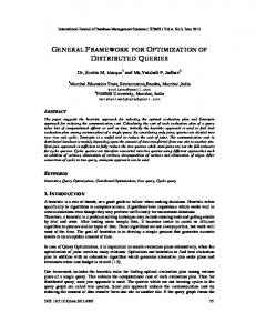
teresting correlations (e.g. “What gene produces proteins missing in diabetes patients?”). Currently, such queries are mainly supported through an ftp-grep approach [13] in which users are forced to download archives of all sources and to query locally. This approach is defective in two ways: First, as pointed out by Gray and Szalay [13], an information avalanche is causing the sources to grow exponentially, leading to databases that take weeks to months to download. For instance, Genbank roughly doubles in size every two years, and is expected to hit the terabyte boundary within three years [25, section 2.2.8]. It is known that this deficiency can be overcome by adopting a distributed, federated architecture where sources cooperate to answer queries and where downloading is hence no longer necessary [13]. Second, users must be knowledgeable of all sources that potentially contribute to the desired answer of a correlation query. To illustrate, consider a biologist looking for Genbank genes that are linked to SwissProt ‘Fly’ proteins with a Go molecular function ‘f ’ and Enzyme description ‘d’. Available to the biologist are the relational tables from the sources and mapping tables that provide the semantic glue to relate them [10, 18]. In its most basic version as used in this article, a mapping table is nothing more than a n-to-n binary relation over the keys of the participating source tables. Figures 1(d)–1(f) show sample mapping tables for the simplified sample instances in Figure 1(a)–1(c) of some of the biological sources mentioned earlier. There, for example, Genbank gene 4763 is directly connected to SwissProt protein O00662, while Genbank gene 768272 is indirectly connected to SwissProt protein Q9Z167 through the link with PubMed article 18022237. The mapping tables are usually stored along with the regular tables at the corresponding sources and are widely used in biology1 . For instance, Figure 1(g) shows a graph in which there is an edge between two sources whenever we found actual mapping tables between them. Using the mapping tables, the query above can be expressed by means of the select-project-join expression ` πgid Genbank 1 MGen,Swiss 1 σspecies =fly (SwissProt) 1 MSwiss,Go 1 σfunc=f (Go) 1 MSwiss,Enz ´ 1 σdesc=d (Enzyme) ,
(Q1 )
where MGen,Swiss , MSwiss,Go , and MSwiss,Enz denote the mapping tables between Genbank and SwissProt; SwissProt and 1
Although mapping tables may seem difficult to maintain at first sight as they need to be created manually by domain specialists, recent work has illustrated how mapping tables can be managed semiautomatically [18].
title Genetic predisposition... Neurofibromatosis: novel... Neuroprotective Effects... Protein phosphatase subunit...
(c) PubMed
pubid 18021924 18022237
pid O00662 Q9Z176
table (f) Mapping between PubMed and SwissProt
OMIM Genbank PubMed
Go
Genbank
SwissProt
SwissProt
Enzyme
Go [func=f ]
(g) Existing mapping tables
[spec=fly] Enzyme [desc=d]
(h) Example exploratory query
Figure 1: Sample instances, mapping tables, and an exploratory query. Go; and SwissProt and Enzyme, respectively. This only returns genes that are directly linked to SwissProt fly proteins with Go function f , however. For genes that are indirectly linked, for example through some common PubMed article, separate expressions like ` πgid Genbank 1 MGen,Pub 1 PubMed 1 MPub,Swiss 1 σspecies=fly (SwissProt) 1 MSwiss,Go 1 σfunc=f (Go) ´ 1 MSwiss,Enz 1 σdesc=d (Enzyme) , (Q2 ) are necessary since MGen,Swiss need not contain all information derivable from MGen,Pub and MPub,Swiss . This is clear from Figure 1, for example where gene 768272 is not directly linked to protein Q9Z167 in MGen,Swiss although it is indirectly linked through PubMed article 18022237 in MGen,Pub and MPub,Swiss . Enumerating all expressions like (Q2 ) is impractical, however, as (1) the number of paths between Genbank and SwissProt may be too large to enumerate manually and (2) the biologist must know the whole network of sources and mapping tables to express her query, a rather ominous requirement in the Internet era where new sources are easily added. For instance, at the beginning of 2008 there were 1078 major molecular biology databases, 110 more than in the beginning of 2007 [12]. Exploratory queries. While the information avalanche problem disappears in the federated architecture setting, the need for complete user knowledge persists. We therefore propose exploratory queries. An exploratory query takes the form of a tree with nodes representing sources and two kinds of edges: direct edges (depicted as single lines) indicating that the sources must be directly linked through some mapping table, and path edges (depicted as double lines) indicating that the sources must be linked through a path of alternating sources and mapping tables. To illustrate, Figure 1(h) shows the exploratory query corresponding to our biologist’s original intent. Due to the declarative nature of exploratory queries, users need only specify local constraints on the sources of interest, and an intent of how these sources should be linked. They need not be aware of other sources, nor of the mapping tables needed to link them. Exploratory query optimization. Of course, actually evaluating an exploratory query requires the evaluation of many concrete queries. To evaluate the query in Figure 1(h), for example, we need to evaluate (Q1 ) and (Q2 ), among others. Sequentially evaluating these queries clearly leads to redundant computation and communication (e.g., subquery
17
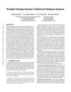
σspecies=fly (SwissProt) is executed multiple times). Since the ratio of communication time to I/O time in a wide area network (WAN) can be of the order of 20:1 [27], it is especially important to minimize the amount of communicated data and to share as much as possible the communication of common subresults. It is this multi-query optimization problem that forms the focus of this article. In particular, we show that the problem of finding an exploratory query evaluation plan that maximizes sharing is np-hard. In response, we optimize an exploratory query E in two steps. In the first step, we generate the concrete queries Q1 , . . . , Qk necessary to evaluate E, and determine optimal evaluation plans for each Qi individually. In the second step we use heuristics to combine these individual plans in a single combined plan. (We discuss each step in more detail in the following paragraphs.) We emphasize that while exploratory query optimization is inherently a multi-query optimization (MQO) problem, existing MQO techniques are unsuitable in our context. Indeed, as further detailed in the Related Work section, they scale only to a small (i.e., 10–15) number of queries whereas in large source networks a single exploratory query may yield hundreds of concrete queries. Moreover, the existing techniques mainly focus on traditional (disk I/O based) optimization instead of communication-based optimization. Hence, while earlier research has shown that combining optimal single-query plans often yields suboptimal multi-query plans with regard to disk I/O cost [31], our experiments show that single-plan combination is not only successful with regard to communication cost, but also scales to thousands of queries. Single plan generation. An evaluation plan for a single concrete query specifies the direction and order in which sources communicate. Figure 2 for example, shows two evaluation plans P1 and P2 for (Q1 ), where edge labels indicate the order of communication. So, in P1 , Go and Enzyme compute in parallel the goids with function f and the eids with description d and send them to SwissProt. SwissProt joins the received ids with MSwiss,Go and MSwiss,Enz respectively to determine which fly pids it should send to Genbank. From these pids and MGen,Swiss , Genbank derives the gids to output. In P2 on the other hand, the order of communication is different. Enzyme first sends to SwissProt the eids with description d. SwissProt joins these with MSwiss,Enz , selects the corresponding fly pids from the result, caches them temporarily, and sends them to Go. Go joins the received pids with MSwiss,Go and returns to SwissProt the matching goids with function f . SwissProt joins the received goids
Genbank
Genbank Genbank SwissProt 1 Go [func=f ]
Genbank
2 [spec=fly] SwissProt 1 3 Enzyme [desc=d]
(a) P1
Go [func=f ]
2
4 [spec=fly] SwissProt 1 1 Enzyme [desc=d]
(b) P2
Go [func=f ]
Genbank
3 PubMed 2 [spec=fly] SwissProt 1
3 PubMed 2 [spec=fly] 1
Enzyme [desc=d]
Enzyme [desc=d]
Genbank 3 2 PubMed SwissProt [spec=fly] SwissProt 2 1 1 1 [spec=fly] 1 Go Enzyme Go [func=f ] [desc=d] [func=f ] Go [func=g]
(c) P3
(d) P4
(e) C1
Figure 2: Evaluation plans and combined evaluation plans. with MSwiss,Go , selects the corresponding fly pids from the result, and intersects them with the pids cached earlier in order to send the correct result to Genbank. Note that the communication cost of P2 is lower than the cost of P1 if the number of ids sent from SwissProt to Go and from Go back to SwissProt in P2 is less than the number of ids sent from Go to SwissProt in P1 . Hence, as in classical query processing, the order in which subresults are joined can have a huge impact on the overall (communication) cost. As this example illustrates, computing the optimal plan for a single concrete query is far from easy. In fact, for arbitrary cost estimation functions, the problem is known to be np-hard [36]. We show that optimal plans for a single concrete query can be computed in time quadratic in the size of the query using a cost estimation function inspired by Stocker et al. [34]. This function is very suited for optimization in loosely collaborating environments, as it does not require detailed statistics to be globally available. Combined plan generation. Intuitively, a combined evaluation plan is an evaluation plan that consists of multiple ordinary evaluation plans. These plans execute in parallel, but share communication as indicated by the combined plan. To illustrate, consider plan P1 for (Q1 ) and plan P3 for (Q2 ) as shown in Figure 2. When executed independently, the intermediate results σfunc=f (Go) and σdesc=d (Enzyme) would be transmitted twice. In the combined plan C1 in Figure 2(e), in contrast, these results are only transmitted once. (The dotted lines indicate for which edges of P1 and P3 communication should be shared.) Combined evaluation plans can also take into account that intermediate results do not coincide completely but have a high overlap. To illustrate, consider plans P1 and P4 in Figure 2. Although Go is filtered by σfunc=f in P1 and by σfunc=g in P4 , a combined plan containing P1 and P4 can still indicate that the communication of these results to SwissProt should be shared. In that case the corresponding ids are transmitted to SwissProt in such a way that shared ids are transmitted only once. Similarly, SwissProt in P1 can share communication to Genbank with SwissProt in P4 . This is especially effective when the results have significant (expected) overlap. As these examples indicate, computing a combined optimal plan is even more challenging than the single-query case. Indeed, we prove that the problem is np-hard, even for the cost estimation function mentioned above for which computation of a single optimal plan is in quadratic time. In response, we propose two efficient heuristics that combine individual plans by looking for structural and semantic similarities. Our first heuristic, levelwise merging, operates by looking for local similarities. Our second heuristic, alignment, is based on a heuristic for solving the multiple partial order alignment problem in Computational Biology [17] and intuitively looks for global similarities.
18
Multi-exploratory query optimization. Finally, we investigate how effective the proposed heuristics are for the optimization of multiple exploratory queries. Such optimization is necessary, for instance, to support continuous exploratory queries that are registered once and that need to be re-evaluated when the sources are updated. In this context, we show that a two-stage approach where (1) a combined plan is computed for each exploratory query and where (2) the resulting plans are later combined in a single super-plan, executes faster than the approach where the super-plan is computed directly, while still yielding superplans of the same quality. To summarize our contributions: 1. We introduce the notion of Exploratory Queries (Section 2). We provide an optimization algorithm for single concrete queries that returns optimal plans in quadratic time (Section 3). In strong contrast, we prove the optimization of single exploratory queries to be np-hard (Section 4). 2. In response, we propose two efficient heuristics for exploratory query optimization (Section 4): levelwise merging and alignment, and derive from these heuristics several two-stage heuristics for the optimization of multiple exploratory queries (Section 5). 3. We assess the effectiveness of the proposed heuristics by extending the BioScout-platform [19] (a distributed monitoring system for biological data) with exploratory queries. Our experiments based on this platform (in Section 6) show that alignment is best suited for the optimization of single exploratory queries as it takes the best advantage of the structural similarity of the corresponding concrete queries. The method is less suited for optimization of multiple exploratory queries as in that case the time needed to construct the combined plans becomes a bottleneck, and levelwise merging yields better plans. For multiple exploratory queries, the two-stage heuristic based on levelwise merging is shown to compute combined plans faster than the one-stage levelwise merging, while still yielding plans of the same quality. Finally, we also show levelwise merging and alignment to be suitable methods for multi-query optimization of sets of arbitrary queries, as opposed to sets of queries that implement the same exploratory query and that hence have significantly shared structure. To the best of our knowledge, this makes them the first algorithms for MQO that scale to hundreds of queries.
2.
PRELIMINARIES
Sources. We consider a fixed, finite set of sources S, together with a set of mapping tables [18] that provide the
Genbank PubMed Genbank Go [func=f ]
Genbank PubMed
[spec=fly] SwissProt OMIM [dis=d]
Go [func=f ]
[spec=fly] SwissProt
[spec=fly]
Enzyme [desc=d]
Enzyme [desc=d]
Go [func=f ]
(a) Example EQ (b) CQ for (Q1 ) (c) CQ for (Q2 ) Figure 3: An exploratory query and two concrete queries. semantic glue to relate them. To simplify notation, we assume each source to consist of a single relation whose key in turn consists of a single attribute (the tuple id attribute). In this way, a mapping table between sources R and S is nothing more than a binary n-to-n relation between the keys of R and S, as illustrated in Fig. 1. Let the Data Interconnection Graph DIG(S) of S be the undirected graph over the sources in S in which edges indicate the presence of a mapping table between the corresponding sources. An example is given in Fig. 1(g). If there is a mapping table between R and S, then we denote this table by MR,S . Mapping tables are assumed to be symmetric, and hence MS,R = MR,S . Exploratory queries. Exploratory queries provide a declarative way for stating correlation queries over S without complete user knowledge of DIG(S). Formally, an exploratory query (EQ) E is a tree with two types of edges, direct edges and path edges, whose nodes are labeled by atoms. An atom A is a pair R[F ] consisting of a source name R ∈ S and a filter F (like “func=f ”) specifying the ids to be selected from R. For each direct edge in E there must be an edge between the corresponding sources in DIG(S). Fig. 1(h) and 3(a) show example EQs with direct edges depicted as single lines and path edges depicted as double lines. As mentioned, Fig. 1(h) selects those Genbank genes that are linked through some path in DIG(S) to SwissProt ‘Fly’ proteins with a Go molecular function ‘f ’ and Enzyme description ‘d’. Fig. 3(a), on the other hand, selects those PubMed articles that are directly linked to a Genbank record that is (1) directly linked to OMIM disease d and (2) linked through some path in DIG(S) to Go function f . Concrete queries. The semantics of EQs is formally defined in terms of the concrete queries that implement them. For Fig. 1(h), these include (Q1 ) and (Q2 ) from the Introduction. We find it convenient to also represent concrete queries as trees. Formally, a concrete query (CQ) Q is a tree whose nodes are labeled by atoms such that for each edge in the tree there is an edge between the corresponding sources in DIG(S). In other words, a concrete query is an exploratory query in which no path edges occur. To illustrate, Figures 3(b) and 3(c) show the concrete queries corresponding to (Q1 ) and (Q2 ) from the Introduction. Semantically, a concrete query Q returns a set of tuple ids. In particular, it returns the set res(r) with r the root node of Q and res(·) defined as follows. Let w be a node in Q labeled by atom A = R[F ]. Then the set of ids returned by w is inductively given by \ res(w) := πidA (A) ∩ πidA (Mw,v 1 res(v)), v∈children(w)
where we abuse notation and simply write A for the set of tuples returned by applying filter F to R; where idA denotes
19
the key attribute of R; and where Mw,v denotes the mapping table between the sources corresponding to nodes w and v. (This mapping table always exists since each edge in M is required to have a corresponding edge in DIG(S).) Observe in particular that res(w) = πidA (A) when w is a leaf node. We should note that, although for ease of exposition we only consider atoms with equality (e.g., func=f ) and inequality filters (e.g., val > 10) in this article, a filter can be anything that is locally supported by the corresponding source. In particular, it can be an SQL statement involving aggregation such as select id from R where func = f group by species having count(*) > 5. Exploratory query semantics. A concrete query Q is said to implement an exploratory query E if it can be obtained from E by replacing every path edge in E with a simple path allowed by DIG(S). (Recall that a simple path in a graph is a path without repeated nodes.) For example, Fig. 4 shows all possible implementations of the EQ in Fig. 3(a). The semantics of an exploratory query is then defined in terms of its implementations, i.e., res(E) := res(Q1 ) ∪ · · · ∪ res(Qk ), where Q1 , . . . , Qk are all possible implementations of E and where res(Qi ) abbreviates res(root(Qi )). Observe that each concrete query is essentially a selectproject-join expression (possibly with arbitrary atoms in the selection conditions). The exploratory queries are therefore essentially select-project-join-union expressions. Since both concrete queries and exploratory queries are tree-shaped, however, they cannot express cyclic joins [2], and therefore necessarily form a strict subclass of the select-project-join(union) queries. A brief discussion of how our results can be extended to deal with cyclic joins may be found in the full version of this article.
3.
OPTIMIZING CONCRETE QUERIES
Since concrete queries form a particular subclass of the exploratory queries (the ones without path edges), it is instructive to discuss their evaluation and optimization before turning our attention to full exploratory queries. Indeed, concrete query optimization will form a key component of exploratory query optimization, as discussed in Section 4. Evaluation plans. To evaluate a CQ, sources must evaluate atoms; transmit ids to neighboring sources; and translate incoming ids by means of mapping tables. The order and direction in which ids are transmitted is recorded in an evaluation plan (or simply plan for short), of which two examples are shown in Figures 2(a) and 2(b). Formally, a plan on a CQ Q is a directed, connected graph P whose nodes are labeled by atoms and whose edges are strictly ordered. This strict partial order ≺P is required to be total on adjacent edges, i.e., for all edges u → v and v → w either u → v ≺P v → w or v → w ≺P u → v (but not both). As with exploratory and concrete queries, there must be an edge between the corresponding sources in DIG(S) for each edge in P . Finally, a single node root(P ) is distinguished as the root of P . Intuitively, ≺P specifies the order of transmission while root(P ) specifies the node whose ids are to be output. A plan is evaluated as follows. Let src(v) stand for the source corresponding to node v. During evaluation P computes, for every node v, a set of tuple ids res(v). This set
PubMed PubMed Genbank PubMed Genbank
[spec=fly]
Genbank
OMIM [dis=d]
[spec=fly]
OMIM
Genbank
SwissProt
PubMed
[spec=fly]
Genbank
PubMed OMIM [dis=d]
PubMed
SwissProt
SwissProt
[spec=fly]
OMIM
PubMed
OMIM [dis=d]
OMIM
Genbank
[spec=fly]
Enzyme
PubMed OMIM [dis=d]
SwissProt
SwissProt
[spec=fly]
PubMed
OMIM [dis=d]
SwissProt
OMIM [dis=d] Go [func=f ]
Go [func=f ]
Go [func=f ]
Go [func=f ]
Go [func=f ]
Go [func=f ]
(a)
(b)
(c)
(d)
(e)
(f)
Figure 4: Concrete queries for the exploratory query in Fig. 3(a) is stored at src(v), and initially consists of the ids returned by the atom A at v, i.e., initially res(v) := πidA (A). When v → w is an edge without predecessor in ≺P , src(v) sends src(v) n Mv,w to src(w). In other words, src(v) sends to src(w) those ids in res(v) that are linked to a tuple in src(w). On reception, src(w) updates res(w): res(w) := res(w) ∩ πidw (Mw,v 1 res(v)), and deletes v → w from P and ≺P , hence enabling other edges to “execute”. Evaluation stops when P has no more edges, at which point res(root(P )) is output. In what follows, we will simply write res(P ) for this output. For example, in the plan P2 shown in Fig. 2(b), Enzyme computes the eids with description d and sends them to SwissProt. (For convenience we have labeled edges in Fig. 2 that are incomparable according to ≺P with equal natural numbers, whereas the other edges are labeled with natural numbers respecting the order in ≺P .) Let vR be the node in P2 with source name R. On reception, SwissProt updates res(vSwissProt ) to πpid (σspec=fly (SwissProt)) ∩ πpid (MSwiss,Enz 1 res(vEnzyme )), and transmits to Go. Go in turn updates res(vGo ) to πgoid (σfunc=f (Go)) ∩ πgoid (MSwiss,Go 1 res(vSwissProt )), and transmits back to SwissProt who updates res(vSwissProt ) := res(vSwissProt )∩πpid (MSwiss,Go 1 res(vGo )). After reception of the updated res(vSwissProt ), Genbank derives the gids to output: res(Genbank) := πgid (Genbank) ∩ πgid (MGen,Swiss 1 vSwissProt ). It is important to note that there can be multiple edges executing simultaneously in a plan. In Fig. 2(a), for example, Go and Enzyme compute and send in parallel the goids with function f and the eids with description d. SwissProt receives both sets of ids and computes πpid (σspec=fly (SwissProt) ∩ πpid (MSwiss,Go 1 res(vGo )) ∩ πpid (MSwiss,Enz 1 res(vEnzyme )) as its final value for res(vSwissProt ). We also note that sources (like Go) always send their own ids to other sources (like SwissProt), and it is the responsibility of the receiving source (SwissProt) to use a mapping table (MSwiss,Go ) to map the received ids to its own ids. Alternatively, Go could have used MSwiss,Go first to send pids to SwissProt, instead of goids. Since in practice the average fan-out of the mapping tables is rather large (see Fig. 7), the latter strategy generates more traffic however, and therefore we opt for the former. The transmission cost of a plan P is the total number of
20
ids transmitted during P ’s evaluation. That is, X cost(P ) := #(v → w), v→winP
where #(v → w) denotes the size of the semijoin res(v) n Mv,w at the time when v → w executes. Optimization. Say that a plan P is a plan for a CQ Q if res(P ) = res(Q) on all possible source relation instances and mapping tables. As usual, the goal of query optimization is to find a plan P for a given CQ Q such that cost(P ) is minimal among all possible plans for Q. Since in general there are infinitely many such plans and since the cost of a plan is unknown until after its evaluation, an optimizer in practice will generate only a finite set of candidate plans for Q and pick one with minimal estimated cost according to some suitably chosen cost estimation method. In this section, we restrict ourselves to those candidate plans built from the nodes in Q that can transmit ids only from child nodes in Q to their parents in Q and vice versa, and we use a particular cost estimation method that allows computation of a candidate with minimal estimated cost in quadratic time. We should stress, however, that our techniques in Section 4 for combining plans of single CQs into plans for EQs are independent of the way in which the single plans are computed. In particular, our combination techniques work equally well on single plans that contain more nodes than Q; on single plans in which ids can also be transmitted between, say, ancestors and descendants (although such transmissions only rarely yield a plan for Q, see the full version of this article); and on single plans that are optimal under some other cost estimation method. Definition 1. A plan P is a candidate of a CQ Q if the nodes of P are the same as the nodes of Q (including labels); root(P ) = root(Q); and the edges of P are a subset of {v → w, w → v | v parent of w in Q}. For example, both P1 and P2 in Fig. 2 are candidate plans for Q1 in Fig. 3(b) while P3 in Fig. 2 is not since its nodes are different than those of Q1 . Observe that cost estimation for a candidate of Q boils down to the estimation of #(v → w), the size of res(v) n Mv,w when v → w executes in P . Since res(v) is defined by an ordinary relational algebra expression, one can use the traditional (distributed) size estimation functions based on join selectivities [27] or histograms [24] for this purpose. In that case, however, computing the candidate plan with the least estimated cost is known to be np-hard [36]. In contrast, the following size estimation function, inspired by Stocker et al. [34], allows such plans to be computed in quadratic time. Essentially, Stocker et al. propose to conservatively estimate the size of an intersection R1 ∩· · ·∩Rn by the minimum
of the cardinalities |R1 |, . . . , |Rn |. Since in our context the set of ids transmitted from src(v) to src(w) when v → w executes in a plan P consists of the ids satisfying the atom A at v intersected with the translated ids received from all incoming edges u → v ≺P v → w this yields the following estimation est(v → w) of #(v → w): est(v → w) := min{est(A), est(u → v) × αu,v | (u → v) ∈ P, (u → v) ≺P (v → w)}. Here, est(A) with A = R[F ] estimates the number of tuples in R satisfying filter F (this estimation can be obtained, for example, by contacting the source R), and αv,w denotes the average fan-out of v-ids in Mv,w , αv,w := avg{|πidw σidv =i (Mv,w )| : i ∈ πidv (Mv,w )}. Observe that the direction is important here, αv,w 6= αw,v . Although est(v → w) depends on the estimations est(u → v) of all predecessor edges u → v ≺P v → w, this definition is not cyclic since ≺P is a strict order. Therefore, est(e) for every edge e in P can be computed by following the order ≺P . The estimated transmission cost ecost(P ) of P is simply the sum of all est(v → w). Say that P is optimal for a CQ Q if (1) P is a candidate of Q; (2) P is a plan for Q; and (3) there is no other candidate plan for Q with smaller estimated cost. Example 1. Assume est(Enzyme[dis=d]) = 5, est(Go [func=f ]) = 75, est(SwissProt[spec=fly]) = 1000, and est(Genbank) = 50 × 106 . Assume that α is as follows v Genbank SwissProt SwissProt
w SwissProt Go Enzyme
αv,w 3 1.5 3
αw,v 2 3.5 2.5
w SwissProt Go SwissProt Genbank
1. downward edges ending in a node v are evaluated before all edges leaving v, i.e., for all u → v in D and all v → w in Q ] D we have (u → v) ≺P (v → w); 2. all edges u → v in Q for which there is no corresponding downward edge v → u in D are evaluated before all downward edges v → w in D leaving v: (u → v) ≺P (v → w); and 3. all edges u → v in Q are evaluated after all edges w → u in Q: (u → v) ≺P (w → u). (Here, root(Q ] D) = root(Q).) For example, if Q1 is the CQ shown in Fig. 3(b), then Q1 ] {vGo → vSwissProt } yields the plan P2 from Fig. 2(b). Let Q|w stand for the subtree of Q rooted at node w in Q, and let up(v) stand for the estimated size of res(v) when we evaluate Q in a bottom-up manner: up(v) := min{est(A), up(w) · αw,v | w ∈ children(v)}.
Then we estimate as follows for P2 from Fig. 2: v Enzyme SwissProt Go SwissProt
Algorithm 1 GenDown Input: CQ Q and number n Output: a set of downward edges for Q 1: let v be the root of Q 2: initialize the result D to the empty set 3: for every child w of v` do ´ ↓↑ 4: Dw := GenDown Q|w , n × αv,w ` ´ ↑ 5: Dw := GenDown Q|w , up(w) ↓↑ 6: c↓↑ w := n + ecost(Q|w ] Dw ) + n · αv,w ↑ ↑ 7: cw := ecost(Q|w ] Dw ) + up(w) ↑ 8: if c↓↑ w < cw then ↓↑ 9: add all edges in Dw ∪ {v → w} to D 10: else ↑ 11: add all edges in Dw to D 12: return D
Hence ecost(P2 ) = 48.75. A similar reasoning for P1 yields ecost(P1 ) = 92.5. Hence, P2 is preferable over P1 . In contrast to estimation techniques based on histograms, the above size estimation function is particularly suited for optimization in loosely collaborating environments, as it only requires a small number of statistics (namely αv,w and |πidv (Mv,w )|) to be globally available. Algorithm GenDown, shown in Algorithm 1 can be used to compute an optimal plan for a given CQ. Essentially, it computes the set of “downward” edges v → w from parent nodes v in Q to child nodes w that, when added to the bottom-up evaluation plan of Q consisting solely of Q’s nodes and edges, yields an optimal plan for Q. To formalize this claim, we introduce the following definitions. Let a downward edge for Q be an edge v → w over the nodes in Q for which w is a child of v in Q. Let D be a set of downward edges for Q and define Q ] D to be the plan P for Q obtained by adding all edges in D to Q such that:
21
In particular, up(v) = est(A) for leaf nodes. Given a CQ Q and a number n, GenDown now operates as follows. For every child node w of Q’s root v, GenDown recursively computes two sets of downward edges in lines 4 and 5: the ↓↑ set Dw for the case where we would add the downward edge v → w and the set Pw↑ for the case where would not. ↓↑ ↑ Based on the estimated costs of Q|w ] Dw and Q|w ] Dw , GenDown estimates in line 6 the gain of adding v → w to the final plan and makes its decision accordingly in the following lines. We show in the full version of this paper: Theorem 1. If Q is a CQ without redundant nodes, then Q ] GenDown(Q, up(root(Q)) is an optimal plan for Q. Moreover, GenDown runs in time quadratic in the number of edges in Q. Here, a node n is said to be redundant in Q if Q is equivalent to the query obtained by removing n and all of its descendants. For instance, the second Go node in Fig. 5 is redundant as this CQ is clearly equivalent to the CQ in Fig 3(b) without this node. Although redundant nodes can be identified and removed in ptime when containment of all mentioned atoms is decidable in ptime (see the full version of this article), this quickly becomes undecidable for arbitrary atoms [2]. Even in the latter case, however, Theorem 1 shows how to compute optimal plans for Q modulo the removal of redundant nodes. In contrast, computing the
Genbank SwissProt Go [func=f ]
[spec=fly]
Go
Enzyme [desc=d]
Figure 5: A concrete query with redundant node. optimal plan using the traditional size estimation techniques is np-hard, even for CQs without redundant nodes [36]. Example 2. With the same parameters as in Example 1, GenDown(Q, up(root(Q)) yields {vGo → vSwissProt }, which results in the optimal plan P2 in Fig. 2(b).
4.
OPTIMIZING EXPLORATORY QUERIES
To evaluate exploratory queries, sources again evaluate atoms; transmit ids to neighboring sources; and translate incoming ids by means of mapping tables. Since EQs in general have many implementing concrete queries however (as shown in Figure 4), the transmission of some intermediate results can be merged. The order and direction in which ids are transmitted and how they should be merged is recorded in a combined evaluation plan (or simply combined plan for short). Combined evaluation plans. Formally, a combined plan C consists of a set of pairwise node-disjoint plans P1 , . . . , Pn , together with an equivalence relation ≡C over the edges in P1 , . . . , Pn (called the merging relation of C) such that • only compatible edges are merged: if (v → w) ≡C (v 0 → w0 ) then src(v) = src(v 0 ) and src(w) = src(w0 ); • the ordering of the edges is respected: if e ≡C f , e0 ≡ f 0 and e ≺Pi e0 for some i, then f 0 6≺Pj f for all j. Figure 2(e) shows an example combined plan in which merged edges are linked by dotted lines. A combined plan evaluates all the Pi in parallel, and outS puts n i=1 res(Pi ) as its final result (we denote this set simply by res(C) in what follows). However, merged edges execute synchronously. In particular, an edge v → w can only execute when all v 0 → w0 ≡C v → w are ready to execute. Since all such edges are compatible (i.e., src(v) = src(v 0 ) and src(w) = src(w0 )), the transmission of their set of ids from src(v) to src(w) can be combined. Several approaches exist to reduce data transfer in this case. For instance, when e1 ≡C e2 ≡C e3 ≡C e4 are merged edges where e1 transmits the id {a}, e2 transmits {b}, e3 transmits {a, b}, and e4 transmits {a}, then one can simply group over the ids, and transmit {(a, 1, 3, 4), (b, 2, 3)} instead. Here the ‘1’ indicates that the id is in the result of e1 , the ‘2’ indicates that the id is in the result of e2 , and so on. This simplistic scheme already results in 20% savings in transmission costs. More advanced compression methods may increase these savings even further. Optimization. Let plans(C) denote the set of plans that C is composed of and let E be an exploratory query. We say that C is a combined plan for E if for every implementation Q of E there exists a plan P ∈ plans(C) that outputs res(Q) and conversely for every plan P ∈ plans(C) there exists an implementation Q of E such that P outputs res(Q). Clearly, if C is a combined plan for E then res(C) is guaranteed to be equal to res(E).
22
Similar to CQ optimization, the goal of EQ optimization is to find a combined plan C for a given EQ E such that cost(C) is minimal among all plans for E. In this sense, Theorem 2 below stands in strong contrast to Theorem 1: it shows that computing optimal combined plans for EQs is much harder than computing optimal plans for CQs. Specifically, adapt the cost estimation method of Section 3 to combined plans as follows. Let E be a set of compatible edges over C. Let compr (E) be a function that estimates the compression ratio achieved by combining the transmission of all edges in E under the particular compression method used (0 < compr (E) ≤ 1) . The estimated number of transmitted ids when all the edges in E execute simultaneously is then defined as X est(E) := compr (E) · est(v → w), v→w∈E
where est(v → w) is the estimated number of ids transmitted from v to w in the plan Pi to which v → w belongs, as defined in Section 3. The estimated cost ecost(C) is then simply the sum of all estimations of synchronously executing edges. That is, if {E1 , . . . , En } is the set of all equivalence classes of ≡C , then ecost(C) := est(E1 ) + · · · + est(En ). In the full version of this paperwe show by a reduction from the Shortest Common Supersequence problem [29]: Theorem 2. Given a number k, an EQ E, and parameters for the cost estimation method, deciding whether there is a combined plan C for E with ecost(C) ≤ k is np-complete. The corresponding optimization problem is hence also nphard. In view of this negative complexity result, we will refrain from generating combined plans for EQs directly. Rather, given a EQ E we first compute the concrete queries Q1 , . . . , Qk implementing E and determine optimal plans for each Qi individually. We then use the heuristic below to construct a merging relation ≡C on the edges of these plans, hence obtaining a combined plan.
4.1
Levelwise merging
Our first heuristic operates by looking for local similarities between edges. In particular, it merges edges in a set of plans P only if they have almost the same level, where the level of an edge e in Pi ∈ P is defined as level (e) := 1 + max{level (f ) | f ≺Pi e}. In particular, level (e) = 1 if there is no edge f with f ≺Pi e. To illustrate, the level of vEnzyme → vSwissProt in Figure 2(b) is 1, the level of vSwissProt → vGo is 2, and so on. Intuitively, the level of an edge measures how early or how late the edge executes in Pi , where edges with a low level execute early and edges with a high level execute late. The motivation for merging an edge only with edges that have a similar level is the following. Consider an edge e in a plan Pi ∈ P and suppose that there are two candidate edges f1 and f2 in a plan Pj that we can merge e with such that level (e) ≈ level (f1 ) but level (e) level (f2 ). Since merged edges must respect the order in ≺Pi and ≺Pj , every successor e0 of e in Pi (with e ≺Pi e0 ) can only be merged to the compatible edges f 0 in Pj with level (f 0 ) > level (f1 ) if we merge e with f1 . If on the other hand, we merge e with f2 then every such successor can only be merged to the compatible edges f 00 in Pj with level (f 00 ) > level (f2 ). Since level (f1 ) ≈ level (e) level (f2 ), we intuitively expect there
to be significantly more such f 0 than f 00 . Therefore, it is preferable to merge e with f1 . When we have several candidate edges to merge an edge v → w with, we intuitively expect the overlap of transmitted ids to be the largest for those edges v 0 → w0 whose atom A0 at v 0 is the most similar to the atom A at v. In order to assess this similarity, we assume given a function sim(A, A0 ) with 0 ≤ sim(A, A0 ) ≤ 1 that encodes available domain knowledge and estimates the overlap between A and A0 . For example, if all proteins with function f1 are guaranteed to also have function f2 , but not f3 , then sim(Go[func = f1 ], Go[func = f2 ]) will be higher than sim(Go[func = f1 ], Go[func = f3 ]). Even when such domain knowledge is not available, sim can syntactically inspect A and A0 to estimate similarity. In our experiments, for example, we have taken sim(A, A0 ) = 1 if A and A0 are guaranteed to select the same ids due to a syntactic containment check, and sim(A, A0 ) = 0 otherwise. The heuristic based on these observations, called levelwise merging, is shown in Algorithm 2. Starting from the initial relation that merges no edges (i.e., e ≡C f iff e = f ), levelwise merging considers the plans in P one by one and refines ≡C . To ensure that this refinement respects ≺P of the plan P under consideration, a queue Q is used. Initially (line 4), Q is populated with the “initial” edges e in P that have no predecessor d ≺P e. For every edge e in Q, levelwise merging then considers those compatible edges f (denoted by e ∼ f ) occurring at level i, i + 1, . . . , i + k that have already been processed. Here, k is an input parameter that determines when edges have a “similar” level, and i = 1 + max{level (d0 ) | d ≺P e, d0 ≡C d} ensures that if e is merged with one of the considered f , then ≺P will be respected. Let [f ] denote the equivalence class of f w.r.t. ≡C . The benefit gained from fusing e with all edges in [f ] is measured as a combination of the expected similarity of combined atoms (higher is better) and the level of [f ] (lower is better). We introduce some notation to define this. Let atoms([f ]) be the multiset consisting of the atoms labeling v, for every (v → w) ∈ [f ]. Let sim(A, atoms([f ])) denote the average similarity of A with regard to the atoms in atoms[f ]: P B∈atoms([f ]) sim(A, B) , sim(A, atoms([f ])) := n where n is the cardinality of the multiset atoms([f ]). Finally, let level ([f ]) = max{level (f 0 ) | f 0 ≡C f }. The score of fusing e to all edges in [f ] is then given by score(e, [f ]) := b1 ×sim(Ae , atoms([f ]))−b2 ×(level ([f ])−i), where 0 ≤ b1 , b2 ≤ 1 are parameters that may be used to bias the score towards similarity rather than level-differences or vice-verse (b1 + b2 = 1), and Ae is the atom at v in e = v → w. In lines 9 − 11, levelwise merging picks a candidate with maximum score (if it exists), and merges accordingly. Finally, e is marked as processed in line 12, and all unprocessed immediate successors of e (the edges f 6∈ D ∪ Q with e ≺P f and no f 0 such that e ≺P f 0 ≺P f ) are added to Q in line 13. Example 3. As a simple illustration of levelwise merging, consider the case where P consists of the plans P1 and P3 in Fig. 2 and suppose that P1 is processed before P3 . Then in the processing of P1 , no edges are merged since all edges of P1 are only compatible with themselves. When
23
Algorithm 2 levelwise merging Input: a set of plans P, a parameter k Output: a fusion relation ≡C 1: Init ≡C to the identity on edges in P 2: Init set of processed edges D ← ∅ 3: for every plan P in P do 4: Init queue Q ← initial (P ) 5: while Q is not empty do 6: e ← pop(Q) 7: i ← 1 + max{level (d0 ) | d ≺P e, d0 ≡C d} 8: Can ← {[f ] | f ∈ D, f ∼ e, i ≤ level (f ) ≤ i + k} 9: if Can 6= ∅ then 10: pick [f ] ∈ Can with max score 11: merge e with every f 0 ∈ [f ] by setting e ≡C f 0 12: add e to processed edges D 13: add unprocessed immediate successors of e to Q 14: Return ≡C
P3 is processed, there is a single compatible candidate for vEnzyme → vSwissProt , namely the corresponding edge in P1 . These edges are therefore merged. Likewise, there is a single compatible candidate for vGo → vSwissProt , namely the corresponding edge in P1 . The other edges in P3 have no compatible edges in P1 , and the resulting combined plan is hence the one in Fig 2(e).
4.2
Partial Order Alignment
Our second heuristic operates by looking for global similarities and is based on an existing heuristic to solve the multiple partial order alignment problem in Computational Biology [17]. In this problem, one is given a set S; a set {O1 , . . . , On } of strict partial orders over S; and a set F ⊆ S × S of possible fusions and is asked to construct a minimal common supergraph for O1 , . . . , On using only fusions in F . To illustrate the concept of a common supergraph, a small example is given in Figure 6 where Figure 6(c) shows a common super graph for O1 and O2 given in Figure 6(a,b). In particular, the nodes in the supergraph are sets of elements from S where an element s can occur at most once in a set in the supergraph, and where distinct s1 and s2 can occur in the same set only if F (s1 , s2 ). Furthermore, all edges in O1 , . . . , On must have corresponding edges in the supergraph. Finally, the supergraph must be acyclic. For instance, the particular solution in Figure6(c) is obtained by applying the node fusions {(a1 , a2 ), (b1 , b2 ), (c1 , c2 ), (e1 , e2 )}. Now clearly, if we take (1) S to be all edges in a set of plans P = {P1 , . . . , Pn }; (2) O1 , . . . , On to be ≺P1 , . . . , ≺Pn , respectively; and (3) construct F such that F (e, f ) if and only if e and f are compatible edges, then a solution to the multiple partial order alignment problem also gives us a fusion relation ≡C . Finding the minimal common supergraph (i.e., the common supergraph for which some measuring function yields a minimal result) is np-complete, however, and for this purpose a heuristic ppoa has been developed [17]. We refer to [17] for the details of this heuristic, but adapt it to our setting by considering a fine-grained scoring mechanism that incorporates the similarity of atoms, similar in spirit to the scoring mechanism used for levelwise merging. In particular, the score of aligning f to all edges in a set of edges E is defined as score(e, E) := ` ´ b1 × sim(Ae , atoms(E)) − b2 × level (E) − level (e) ,
a1
c1
d1
b1
b2 e1
a2
c2
e2
are found for a query, the owner is notified. To assess the algorithms presented in this paper, we extended BioScout’s functionality with exploratory queries.
g2
f1 (a) O1 a1 , a2
(b) O2 c1 , c2
b1 , b2
d1 e1 , e2
g2
f1 (c) minimal common super graph of O1 and O2
Figure 6: A minimal common super graph. Algorithm 3 alignment/levelwise merging Input: a set of EQs E = E1 , . . . , En Output: a combined plan C for E 1: for each E in E do P = plans of the implementations of E 2: 3: C = alignment(P ) 4: add C to C 5: C = levelwisemerging(C) 6: Return C
where 0 ≤ b1 , b2 ≤ 1 are tuning parameters (b1 + b2 = 1), Ae denotes the atom at v in e = v → w, atoms(E) denotes the multiset of atoms labeling v 0 for every v 0 → w0 ∈ E, level (e) is defined as in Section 4.1, and level (E) = max{level (f ) | f ∈ E}. Let alignment denote the resulting algorithm.
5.
OPTIMIZING MULTIPLE EQs
The proposed heuristics of Sections 4.1 and 4.2 can readily be adapted for the optimization of multiple exploratory queries. Such optimization is necessary, for instance, to support continuous evaluation of exploratory queries that are registered once and that need to be re-evaluated when the sources are updated. Given exploratory queries E1 , . . . , Em one can first compute plans P1 , . . . , Pn for all of their implementations, and subsequently compute a merging relation ≡C for them using levelwise merging or alignment. Alternatively, one can apply a two-staged approach: (1) first compute a separate combined plan for each exploratory query; and, (2) subsequently combine these plans into a single combined plan using either levelwise merging or alignment. Of course, in the second phase levelwise merging and alignment need to compute merging relations based on existing merging relations, but they are readily extended to this case. In our experiments, we consider three two-phase strategies. The first two simply consist of applying levelwise merging and alignment in both phases. Since (as we will demonstrate in Section 6) alignment gives better results for a single EQ, we also consider the strategy where in the first phase alignment is applied and in the second phase levelwise merging. Algorithm 3 gives a schematic overview of the latter approach.
6.
EXPERIMENTS
BioScout platform. BioScout is a distributed monitoring system for biological data which we described in [19]. It consists of a relatively small number of sources: the biological sources mentioned in Fig. 1(g). Scientists can register queries which are evaluated periodically. When new results
24
Setup. The experiments were performed on a Pentium IV (3.0 GHz) architecture with 1 GB of internal memory running under Linux 2.6. Figure 7 shows the statistics for (portions of) the databases and mapping tables used in our experiments which were downloaded from the actual biological sources. Specifically, we show the sizes of the databases along with the sizes of some mapping tables in terms of number of tuples. Notice that database sizes vary from a few thousands to millions of tuples and that the same is true for mapping tables. Figure 7(c) depicts the number of distinct ids in the left and right-hand side database of each reported mapping table along with the average fan-out. We stress the importance of these statistics for the estimation of transmission costs. Notice that the tables are not complete, i.e., not every tuple in a database has a corresponding tuple in another database. For example, from the eleven million Genbank gid’s, only seventeen thousand are associated with enzymes. Also the fan-out of tables varies widely from values close to one, to values close to 55. For our experiments, we have generated 500 EQs of varying size (4 to 6 nodes) and shape with at least one path edge, in which all atom filters are conjunctions of the form attrib = value and attrib LIKE value. The resulting EQs correspond to almost 3000 concrete queries. We emphasize that although these EQs are small, the corresponding evaluation plans can be much larger. For example, we encountered plans with up to seventeen edges in our experiments. As briefly touched upon in Section 4, there are various ways to reduce data transfer when transmitting query results over a network. As all of these exploit commonalities of the data in some way or another, we choose to abstract from a concrete compression method and measure in what follows the indicated transmission costs in terms of uniquely transmitted ids. All of our experiments use a value of k = 2 as locality parameter for levelwise merging, and we have taken sim(A, A0 ) = 1 if A and A0 are guaranteed to select the same ids (tested by a mutual containment check on the filters in A and A0 ), and sim(A, A0 ) = 0 otherwise. Experiment 1. The first experiment is designed to validate our heuristics for optimizing a single EQ E. As a baseline, we also provide the transmission cost for the case where all optimal plans of implementations of E are executed sequentially without any merging (we refer to this method as sequential in what follows). Fig. 8(a) shows the total (aggregated) transmission cost for 50 EQs from our pool of queries. Both heuristics significantly reduce communication: on average by 50% with values ranging from as low as 5% to as high as 85% reduction. Low improvements occur when only few ids are transferred (around 20000) while large improvements occur when many ids (around 1 million) are transferred. Furthermore, for each of the 50 EQs, the transmission cost of the plan computed by alignment was always smaller than that of levelwise merging. The improvement varied from 1% to 30% with, as can be derived from Figure 8(a), an average improvement of 10%. This discrepancy can be explained by analyzing the structure of the plans generated by the two heuristics. Figure 8(b) depicts box plots of the number of equivalence classes of ≡C . Clearly, alignment generates smaller plans: fewer equiv-
Figure 8: Results for the optimization of 50 single EQs. alence classes implies more sharing of communication. As a result, the maximum difference in level between merged edges in the same equivalence class is greater for alignment than levelwise merging, as shown in Figure 8(c). Constructing the 50 combined plans was reasonably fast: it took levelwise merging 8.62 seconds, and alignment 10.24 seconds. Experiment 2. The second experiment is designed to validate our approach for optimizing multiple EQs. We have optimized and evaluated three batches of EQs of size 175, 350 and 500 respectively. These correspond to 1000, 2000, and 3000 concrete queries. As baseline we use again sequential which corresponds to no optimization. In addition we use a second baseline called template inspired by approaches like e.g. NiagaraCQ [8] which group queries based on a common expression signature disregarding selection constants. Intuitively, template checks for all plans P and P 0 whether the graph of P is isomorphic to a subgraph of P 0 respecting ≺P . If so, then all edges of P are merged with the corresponding edges in P 0 . The total transmission cost is shown in Figure 9(a) and in more detail for the third batch of EQs with 3000 EPs in Figure 9(b). It becomes apparent that all proposed approaches significantly reduce the transmission cost with repect to both baselines. Further, the transmission costs only increase moderately for increasing number of evaluation plans. Specifically, when tripling the number of evaluation plans (from 1000 to 3000) the transmission costs of sequential, template and levelwise merging increase with 242%, 227% and 55%, respectively. The high transmission cost of template indicates that merging based on subgraph isomorphism is too restrictive for the optimization of multiple EQs. In addition, it stresses that evaluation plans for randomly generated EQs are sufficiently different to warrant more sophisticated approaches like alignment and levelwise merging. A second observation drawn from Fig. 9(b) is that levelwise merging-based methods outperform alignmentbased methods for the optimization of multiple EQs. The reason for this is that levelwise merging merges edges with similar levels from the bottom up. When the number of plans is large and the locality threshold k is low, there will
25
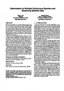
eventually be a phase transition point where there are many (unmerged) edges on the lower levels. After this point, extra edges to be merged almost always find a candidate amongst those present. alignment, in contrast, as already explained in Experiment 1, allows merging of edges with large level differences. As a result, there is less saturation at the lower levels, inhibiting later merging. Finally, one-phase and two-phase levelwise merging are comparably succesful in reducing the total transmission cost (91, 4% versus 91, 1% reduction w.r.t. sequential). Figure 9(c) shows the construction time for computing the combined plan for the different approaches. For the case of 3000 plans, we have omitted for reasons of presentation the outlier construction times of alignment and two-phase alignment, which are around 25000 and 30 000 seconds, respectively. Specifically alignment scales very poorly. The reason is twofold. Since alignment searches for global similarities more and more possible ways of merging edges have to be considered. Furthermore, more time has to be spent computing atom similarities for large number of equivalence classes. levelwise merging, in contrast does scale to large batches of EQs. Furthermore, its two-stage variant constructs the combined plans on average 20% faster, while yielding plans of the same quality. Experiment 3. Our final experiment is designed to validate the behavior of levelwise merging and alignment as suitable methods for multi-query optimization of sets of arbitrary queries, as opposed to sets of queries that implement the same exploratory query and which hence have significantly shared structure. Specifically, for each EQ we randomly choose one concrete query resulting in 500 overall evaluation plans. Figure 10 shows that levelwise merging and alignment also significantly reduce the transmission cost in this unfavorable setup. Both algorithms save around 70% transmission cost compared to sequential, with a small advantage for levelwise merging. As in the previous experiments, the construction time for alignment (1296.17 seconds) is again notably larger than for levelwise merging (157.58 seconds). In summary. alignment is best suited for the optimization of single exploratory queries as it takes the best advan-
Figure 9: Results for the optimization of multiple EQs.
Number of Identifiers
2e+07
1.5e+07
1e+07
5e+06
0 Sequential Alignment Levelwise
Figure 10: Total cost for 500 random plans tage of the structural similarity of the corresponding concrete queries. The method is less suited for multiquery optimization both for exploratory and concrete queries as the construction of the actual combined plan does not scale well to larger sets of queries. levelwise merging is best suited for multiquery optimization of concrete queries (both in terms of transmission cost and in terms of construction time). Moreover, its two-phase variant lw/lw is the best choice for the optimization of multiple EQs because of faster construction time.
7.
RELATED WORK
Distributed databases. Distributed query processing has been investigated since the early days of database systems [21] and the interest is still strong in this area [34]. From the huge literature, most related to ours are the works on the optimization of semi-joins [3, 4], where the objective is also to minimize communication cost among participating sources. In this line of work, [9] only considers chain queries while we consider the more general class of full-reducer tree queries [36]. For this latter class, a number of optimization algorithms have been proposed [28, among others] but they all focus on single-query optimization, while we also consider multi-query optimization. More recently, Stocker et al. [34] have considered generic semi-join optimization techniques. The proposed techniques target a particular class of distributed client-server systems, however, in which clients communicate with servers while servers cannot communicate between themselves. Our work, in contrast, is complimentary as it considers exactly the setting where interserver communication is possible. The difference in the two systems is essential since it influences the evaluation plans considered. Furthermore, we also consider multi-query optimization. From a theoretical standpoint, the problem of optimizing full-reducer tree queries was shown to be np-hard
26
in [36] w.r.t. a cost-model based on (semi)-join-selectivities. Here, we consider a more conservative cost model (c.f. Section 3) motivated by [34], and consider the complexity both for single- and multi-query optimization. Multi-query optimization. In [31], queries (and their plans) are represented as AND-OR DAGs [30] and a family of optimization algorithms is presented to (a) group multiple query DAGs into a single one, by exploiting common query sub-expressions, and (b) determine which common sub-expressions to materialize to reduce the cumulative query evaluation cost (in terms of time). The proposed algorithms are effective for a relatively small number of chain queries and some of the underlying optimization principles there can be found in our work. However, we consider a much larger number of more general queries and focus on minimizing the communication cost. Multi-query optimization is also considered in [35], in the context of sensor networks, but only for aggregation queries, while the techniques in [33] for multi-query optimization are expensive and cannot scale to a large number of queries, as [8] also points out. In [32] an np-hardness result is proved for multi-query optimization for a setting which is entirely different from ours: plans consist of sequences of abstract tasks without any meaning associated to them. In strong contrast, in our setting, every local plan has a clear semantics: it must compute the given query. The hardness result in [32] therefore does not imply our Theorem 2. Scientific Databases. SkyQuery [23] offers subscription of queries over a federation of astronomy databases. The SkyQuery optimizer focuses on minimizing communication cost through a simple strategy that uses performance queries and asks each database for its estimate of data for a given query. Then, databases are ordered in decreasing order of selectivity - the one with least data is the first to execute etc. Currently, SkyQuery does not support more complex (nonchain) plans or multi-query optimization. In [26], a system is proposed to monitor biological data. The queries are similar to ours but their setting is a centralized one where every source communicates only with a central source. Furthermore, it is not the amount of data transfer that is minimized but the total number of different database accesses. BioGuide [6,7] is a system which helps scientists in selecting sources and finding alternate paths between them. Optimization of life science queries in the work of [5] focuses on single queries where the largest set of answers, following alternate paths through the graph connecting the sources, has to be computed at the lowest cost. Data integration systems for the life sciences, like Aladin [22], BioFuice [20], Kleisli [11], Orchestra [14] or DiscoveryLink [15] focus on the seamless
integration of data from heterogeneous sources and on the optimization of single-queries and/or updates. As such, they do not consider scalable multi-query optimization like we do. Peer-to-peer systems. Distributed query processing has also been studied in the context of unstructured p2p systems. Like us, systems like Piazza [16] and Hyperion [18] focus on heterogeneous sources. However, the focus there is on query translation, through mappings, between the sources. Like Hyperion, our work uses data-level mapping between heterogeneous sources. Unlike Hyperion, a distributed query here involves multiple sources, instead of a single source each time. Furthermore, to our knowledge, no work in this area deals with the optimization of distributed queries. Publish-subscribe systems. In publish-subscribe systems, multi-query optimization was only considered in the context of boolean queries. In NiagaraCQ [8], the plans of multiple queries are grouped together if they have common expression signatures, i.e., their plans have common syntactic characteristics. Our work differs since (a) we consider non-boolean queries; and (b) apart from syntactic similarities, our algorithms also take into account the communication cost while computing and merging different plans.
8.
CONCLUSIONS AND FUTURE WORK
We have proposed exploratory queries as a user-friendly means to query large networks of scientific databases for interesting correlations and have proposed several heuristics for the optimization of exploratory queries and the optimization of multiple exploratory queries. This research is part of an ongoing effort to build a distributed querying and monitoring system for biological data called BioScout [19]. For the querying part, we currently support only a small number of sources (namely six), which makes the enumeration of all implementations of an exploratory query manageable. For much larger networks it could be helpful to define a suitable ranking mechanism to avoid brute-force enumeration of paths [5]. For the monitoring part, we support the continuous evaluation of (exploratory) queries. In this context, huge communication gains can be made by caching subresults of previous evaluations and only transmitting differences with these results upon re-evaluation. In future work, we plan to investigate how the present optimization algorithms can be extended to take such caching into account.
9.
REFERENCES
[1] Nucleid acid research database list. http://www.oxfordjournals.org/nar/database/cap/. [2] S. Abiteboul, R. Hull, and V. Vianu. Foundations Of Databases. Addison-Wesley, 1995. [3] P. A. Bernstein and D.-M. W. Chiu. Using semi-joins to solve relational queries. J. ACM, 28(1):25–40, 1981. [4] P. A. Bernstein, et al. Query processing in a system for distributed databases (SDD-1). TODS, 6:602–625, 1981. [5] J. Bleiholder, et al. Query planning in the presence of overlapping sources. In EDBT, p. 811–828, 2006. [6] S. C. Boulakia, et al. Bioguidesrs: querying multiple sources with a user-centric perspective. Bioinformatics, 23(10):1301–1303, 2007. [7] S. C. Boulakia, et al. Path-based systems to guide scientists in the maze of biological data sources. J. Bioinformatics and Computational Biology, 4(5):1069–1096, 2006. [8] J. Chen, D. J. DeWitt, F. Tian, and Y. Wang. NiagaraCQ: a scalable continuous query system for internet databases. In SIGMOD, p. 379–390. ACM, 2000. [9] D.-M. W. Chiu, P. A. Bernstein, and Y.-C. Ho. Optimizing chain queries in a distributed database system. SIAM J. Comput., 13(1):116–134, 1984.
27
[10] S. B. Davidson, G. C. Overton, and P. Buneman. Challenges in integrating biological data sources. J. of Computational Biology, 2(4):557–572, 1995. [11] S. B. Davidson, G. C. Overton, V. Tannen, and L. Wong. Biokleisli: A digital library for biomedical researchers. Int. J. on Digital Libraries, 1(1):36–53, 1997. [12] M. Y. Galperin. The molecular biology database collection: 2008 update. Nucleic Acids Research, 36:D2–D4, 2008. [13] J. Gray and A. S. Szalay. Where the rubber meets the sky: Bridging the gap between databases and science. IEEE Data Engineering Bulletin, 27(4):3–11, 2004. [14] T. Green, G. Karvounarakis, Z. Ives, and V.Tannen. Update exchange with mappings and provenance. In VLDB, p. 675–686, 2007. [15] L. M. Haas, et al. Discoverylink: A system for integrated access to life sciences data sources. IBM Systems Journal, 40(2):489–511, 2001. [16] A. Halevy, Z. Ives, J. Madhavan, P. Mork, D. Suciu, and I. Tatarinov. The piazza peer data management system. IEEE Trans. Knowl. Data Eng., 16(7):787–798, 2004. [17] D. S. Parker Jr. and C. Lee. Pairwise partial order alignment as a supergraph problem. 2003. [18] A. Kementsietsidis, M. Arenas, and R. Miller. Mapping data in peer-to-peer systems: Semantics and algorithmic issues. In SIGMOD, p. 325–336, 2003. [19] A. Kementsietsidis, F. Neven, and D. Van de Craen. Bioscout: A life-science query monitoring system. Demo to be presented at EDBT, 2008. [20] T. Kirsten and E. Rahm. Biofuice: Mapping-based data integration in bioinformatics. In DILS, p. 124–135, 2006. [21] D. Kossmann. The state of the art in distributed query processing. ACM Comput. Surv., 32(4):422–469, 2000. [22] U. Leser and F. Naumann. (almost) hands-off information integration for the life sciences. In CIDR, p. 131–143, 2005. [23] T. Malik et al. Skyquery: A web service approach to federate databases. In CIDR, 2003. [24] M. V. Mannino, P. Chu, and T. Sager. Statistical profile estimation in database systems. ACM Computing Surveys, 20(3):191–221, 1988. [25] NCBI. Genetic sequence data bank release notes, December 2007. ftp://ftp.ncbi.nih.gov/genbank/gbrel.txt. [26] F. Neven and D. Van de Craen. Optimizing monitoring queries over distributed data. In EDBT, p. 829–846, 2006. ¨ [27] M. Oszu and P. Valduriez. Principles of Distributed Database Systems. Prentice Hall, 2nd edition, 1999. [28] S. Pramanik and D. Vineyard. Optimizing join queries in distributed databases. IEEE Trans. Software Eng., 14(9):1319–1326, 1988. [29] K.-J. R¨ aih¨ a and E. Ukkonen. The shortest common supersequence problem over binary alphabet is NP-complete. TCS, 16:187–198, 1981. [30] N. Roussopoulos. View indexing in relational databases. TODS, 7(2):258–290, 1982. [31] P. Roy, S. Seshadri, S. Sudarshan, and S. Bhobe. Efficient and extensible algorithms for multi query optimization. In SIGMOD, p. 249–260. ACM, 2000. [32] T. Sellis and S. Ghosh. On the multiple-query optimization problem. Trans. Knowl. Data Eng., 2(2):262–266,1990. [33] T. K. Sellis. Multiple-query optimization. TODS, 13(1):23–52, 1988. [34] K. Stocker, et al. Integrating semi-join-reducers into state of the art query processors. In ICDE, p. 575–584., 2001. [35] N. Trigoni, Y. Yao, A. J. Demers, J. Gehrke, and R. Rajaraman. Multi-query optimization for sensor networks. In DCOSS, p. 307–321, 2005. [36] C. Wang and M.-S. Chen. On the complexity of distributed query optimization. IEEE Trans. Knowl. Data Eng, 8(4):650–662, 1996.