its parameter-free nature. .... matrices in a parameter-free fashion, i.e. find the clusterings ..... from each domain is treated as one type of objects at the leaf.
PaCK: Scalable Parameter-Free Clustering on K-Partite Graphs Jingrui He∗
Hanghang Tong∗ Spiros Papadimitriou† Tina Eliassi-Rad‡ Christos Faloutsos∗ Jaime Carbonell∗
Abstract Given an author-paper-conference graph, how can we automatically find groups for author, paper and conference respectively. Existing work either (1) requires fine tuning of several parameters, or (2) can only be applied to bipartite graphs (e.g., author-paper graph, or paper-conference graph). To address this problem, in this paper, we propose PaCK for clustering such k-partite graphs. By optimizing an information-theoretic criterion, PaCK searches for the best number of clusters for each type of object and generates the corresponding clustering. The unique feature of PaCK over existing methods for clustering k-partite graphs lies in its parameter-free nature. Furthermore, it can be easily generalized to the cases where certain connectivity relations are expressed as tensors, e.g., time-evolving data. The proposed algorithm is scalable in the sense that it is linear with respect to the total number of edges in the graphs. We present the theoretical analysis as well as the experimental evaluations to demonstrate both its effectiveness and efficiency. 1
Introduction
Complex graphs that express various relationships among objects of different types are rapidly proliferating, largely due to the prevalence of the Web and the Internet. For example, the Resource Description Framework (RDF) [24] aims to express practically all multi-relational data in a standard, machine-understandable form. One of the Web’s creators has even envisioned the Giant Global Graph (GGG) [5], which would capture and represent relationships across documents and networks. In this paper we focus on a simpler but expressive subset of multi-relational data representations. We consider entities or objects of multiple types and allow any pair of types to be linked by a binary relationship. For example, in a publication corpus, papers (one object type) are associated with several other object types, e.g., authors, subject keywords, and publication venues. Given such data, how can we find meaningful patterns and groups of objects, across different types? One approach might be to cluster the objects of each type independently of ∗ Carnegie
Mellon University T.J. Watson Lab ‡ Lawrence Livermore National Laboratory † IBM
the rest. Traditional clustering techniques [13] are designed to group objects in an unlabeled data set such that objects within the same cluster are similar to each other, whereas objects from different clusters are dissimilar. Most clustering algorithms, such as k-means [9], spectral clustering [2] and information-theoretic clustering [11], focus on one-way clustering, i.e. clustering the objects according to their similarity based on the features. However, for sparse relational data, co-clustering or biclustering techniques [18] simultaneously cluster objects of all types and typically produce results of better quality, by leveraging clusters along other types in the similarity measure. Most co-clustering algorithms focus on just two types of objects, typically viewed as either rows and columns of a matrix, or source and destination nodes of a bipartite graph. The information-theoretic co-clustering (ITCC) algorithm [8] was among the first in the machine learning community to address this problem. Follow up work includes [17], [15], and [3]. More recently, algorithms that generalize co-clustering to more than two object types have appeared, such as Consistent Bipartite Graph Co-partitioning (CBGC) [10], spectral relational clustering [16], and collective matrix factorization [20, 21]. These address some of the challenges in mining multi-relational data. However, despite their success, all of these methods require the user to provide several parameters, such as the number of clusters of each type, weights for different relations, etc. We aim to provide a method that can also recover the number of clusters, by employing a model selection criterion based on lossless compression principles. Our starting point is the cross-associations [7] and Autopart [6] methods, both of which are parameter-free and provide the basic underpinnings for the model selection principles we shall employ. However, neither of them apply to multi-relational data. These pose additional challenges, which we address by introducing several new ideas, including exponential cluster splits, cluster merges, and multiple concurrent trials. In this paper we propose PaCK to co-cluster k-partite graphs. Our main contributions in this paper are:
matrix Dij such that the objects within the same clusters are put together. In this way, the matrix Dij is divided into pq smaller blocks, which are referred to as Dij , p = 1, . . . , ki pq and q = 1, . . . , kj . Let the dimensions of Dij be (api , aqj ). p In other words, ai is the number of objects from X i that belong to cluster p, and aqj is the number of objects from X j that belong to cluster q. Table 1 summarizes the notation used in this paper. 2.2 A Lossless Code for Connectivity Matrices. Extensive experiments on both real and synthetic datasets, Suppose that we are interested in transmitting the connectivinclude comparisons to several other methods, validate the ity matrices Dij , i = 1, . . . , m − 1 and j = i + 1, . . . , m. effectiveness of PaCK. We are also given the mapping Φi that partitions the objects The rest of the paper is organized as follows: Section 2 in X i into ki clusters, with none of them empty. Next, we informulates the problem; Section 3 introduces the PaCK troduce how to simultaneously code multiple matrices based search procedure; and Section 4 presents experimental reon the above information. sults; finally, Section 5 reviews related methods and Sec2.2.1 Description Complexity. The first part is the detion 6 concludes. scription complexity of transmitting the connectivity matri2 Problem Formulation ces. It consists of the following parts: In this section, we give the problem formulation of PaCK. 1. Send the number of object types, i.e., log∗ (m), where Similar to cross-associations [7] and Autopart [6], PaCK log∗ is the universal code length for integers.1 This term tries to formulate the clustering problem as a compression is independent of the collective clustering. problem. Unlike cross-associations [7] and Autopart [6], 2. Send Pm the∗ number of objects of each type, i.e., PaCKtries to compress a set of inter-correlated matrices coli=1 log (ni ). This term is also independent of the lectively, as apposed to a single matrix in cross-associations collective clustering. and Autopart. 3. Send the permutations of the objects of the same type Given a set of inter-connected objects of different types, so that the objects Pm within the same clusters are put our goal is to find patterns based on the binary connectivity together, i.e., i=1 ni dlog ki e. matrices in a parameter-free fashion, i.e. find the clusterings Pm 4. Send the number of clusters using i=1 log∗ ki bits. for different types of objects simultaneously so that after re5. Send the number of objects in each cluster. For object arranging, the connectivity matrices will consist of homogetype X i , suppose that a1i ≥ a2i ≥ . . . ≥ aki i ≥ 1. neous, rectangular regions of high or low density. ki Compute X Generally speaking, to achieve this goal, we make use of p a ¯ := ( ati ) − ki + p i the MDL (Minimum Description Length) principle to design t=p a criterion, and try to minimize this criterion greedily. We for i = 1, . . . , m and p = 1, . . . , ki − 1. So altogether describe the criterion in this section and deal with the search the desired quantities can be sent using the following procedure in the next section. number of bits: m kX 2.1 Notation. i −1 X dlog a ¯pi e Given m types of data objects, X1 = i=1 p=1 {x11 , . . . , x1n1 }, . . . , X m = {xm1 , . . . , xmnm }, where pq X i is the ith object type, xij is the j th object of the ith , i = 1, . . . , m − 1, j = 6. For each matrix block Dij th type, and ni is the number of objects from the i type, we i + 1, . . . , m, p = 1, . . . , ki , and q = 1, . . . , kj , send are interested in collectively clustering X 1 into k1 disjoint the number of ones, using dlog(api aqj + 1)e bits. clusters, . . ., and X m into km disjoint clusters. Let 2.2.2 Code for the Matrix Blocks. In addition to the Φi : {1, 2, . . . , ni } → {1, 2, . . . , ki }, i = 1, . . . , m above information, we also need to transmit the matrix pq pq denote the assignments (i.e., mappings) of objects in X i to blocks Dij . For a single block Dij , we can model its the corresponding clusters. elements as iid draws from a Bernoulli distribution with pq pq pq Let Dij denote the ni × nj binary connectivity matrix bias Pijpq = n(Dij , 1)/(n(Dij , 1) + n(Dij , 0)), where pq pq between object types X i and X j , i 6= j, i.e., the element in n(Dij , 1) and n(Dij , 0) are the numbers of ones and zeros the sth row and tth column of Dij is 1 if and only if xis is connected to xjt . 1 log∗ (x) ≈ log (x) + log log (x) + . . ., where only the positive 2 2 2 To better understand the collective clustering, given the terms are retained and this is the optimal length, if we do not know the mappings Φi , i = 1, . . . , m, let us rearrange the connectivity range of values for x beforehand. • PaCK is parameter-free, by employing a simple but effective model selection criterion, which can recover the “true” cluster structure (when known). • We carefully design a search procedure that can find a good approximate solution. • Our algorithms are scalable to large datasets (linear on. number of edges). • We generalize PaCK to tensors.
Symbol m Xi ni ki kiS ki∗ Φi Φi (s) ΦSi Φ∗i Dij Dij {t} api pq Dij pq Dij (s) n(A, u) n(A) Pijpq Pijpq (s) H(Pijpq ) pq Cij pq Cij (s) TD (Φ1 , . . . , Φm )
Table 1: Notations Definition Number of object types The ith object type Number of objects in X i Number of clusters for X i ki in the S th iteration step of PaCK Optimal number of clusters for X i Assignments/mappings of objects in Xi to the corresponding clusters Φi in the sth iteration step of CCsearch Φi in the S th iteration step of PaCK Optimal assignments/mappings of objects in X i to the corresponding clusters ni × nj binary connectivity matrix between object types X i and X j Dij at time stamp t when the relationship between X i and X j is a tensor Number of objects from X i that belong to cluster p Block of Dij that corresponds to the pth cluster in X i and the q th cluster in X j pq Dij in the sth iteration step of CCsearch Number of elements in the matrix/vector A that are equal to u, u = 0, 1 Total number of elements in the matrix/vector A pq Proportion of 1s in Dij pq th Pij in the s iteration step of CCsearch Binary Shannon entropy function with respect to Pijpq pq Coding length required to transmit the block Dij using arithmetic coding pq th Cij in the s iteration step of CCsearch Total coding cost with respect to the mappings Φ1 , . . . , Φm
pq in Dij . Therefore, the number of bits required to transmit this block using arithmetic coding is
that the total coding cost TD (Φ∗1 , . . . , Φ∗m ) is minimized. This problem is NP-hard2 . Therefore, we have designed a pq pq pq greedy algorithm to minimize the total coding cost (EquaCij = C(Dij ) := n(Dij )H(Pijpq ) tion (2.1)). Specifically, to determine the optimal collective pq pq = −n(Dij , 1) log(Pijpq ) − n(Dij , 0) log(1 − Pijpq ) clustering, we must set the number of clusters for each object type, and then find the optimal mappings. These two pq pq pq where n(Dij ) = n(Dij , 1)+n(Dij , 0), and H is the binary components correspond to the two major steps in PaCK: (1) Shannon entropy function. finding a good collective clustering given the number of clus2.2.3 Total Coding Cost. Based on the above discussion, ters of each objective type; and (2) searching for the optimal the total coding cost for the connectivity matrices Dij , i = number of clusters. 1, . . . , m − 1, j = i + 1, . . . , m with respect to the given In this section, we first describe these two steps respecmappings Φi , i = 1, . . . , m is as follows. m m tively, followed by computational complexity analysis for X X the proposed PaCK. TD (Φ1 , . . . , Φm ) := ni dlog ki e + log∗ ki i=1 i=1 3.1 CCsearch kj ki X m kX m−1 m X In CCsearch step, we are given the values of k1 , . . . , km , i −1 X X X p and want to find a set of mappings Φ1 , . . . , Φm that mini+ dlog a ¯i e + dlog(api aqj + 1)e mizes the total coding cost (Equation (2.1)). Note that in i=1 p=1 i=1 j=i+1 p=1 q=1 this case, the first two terms in Equation (2.1) are fixed, and kj ki X m−1 m X X X Pm Pki −1 pq only the remaining three terms ¯pi e, + (2.1) Cij i=1 p=1 dlog a P P P P kj m−1 m ki p q i=1 j=i+1 p=1 q=1 + 1)e and q=1 dlog(ai aj i=1 j=i+1 p=1 P P P P k m−1 m ki pq Pm j ∗ ∗ depend on the mapq=1 Cij Note that we ignore the costs log (m) and i=1 log (ni ), i=1 j=i+1 p=1 pings. Based on our experiments, in the regions where since they do not depend on the collective clustering. 3 Search Procedure in PaCK 2 It is NP-hard since even allowing only column re-ordering for a single The optimal collective clustering corresponds to the number of clusters ki∗ and the mapping Φ∗i for object type X i such connectivity matrix, a reduction to the TSP problem can be found [14].
CCsearch searches for the optimal mappings given the numbers of clusters, the code for transmitting the matrix blocks dominates the total coding cost. Therefore, in CCsearch, we aim to minimize the following criterion: kj ki X m−1 m X X X pq (3.2) Cij
Algorithm 1 CCsearch Input: The connectivity matrices Di,j , i, j = 1, ..., m; the cluster numbers ki , i = 1, ..., m for each type. Output: The cluster assignment Φi for each object type. 1: Let s denote the iteration index and set s = 0. 2: Initialize collective clustering Φ1 (s), . . . , Φm (s). i=1 j=i+1 p=1 q=1 3: Set Φ0i (s) = Φi (s), i = 1, . . . , m. 4: while true do CCsearch (Alg. 1) is an intuitive and efficient alternat5: ### alternate among different types of objects ing minimization algorithm that yields a local minimum of for l = 1, . . . , m do 6: Equation (3.2). 7: ### try to update the clustering for type l Note that CCsearch is essentially a Kmeans-style algo8: for i = 1, . . . , m − 1, j = i + 1, . . . , m, p = rithm [19]: it alternates between finding the cluster centroid 1, . . . , ki , q = 1, . . . , kj do and assigning objects to the ‘closest’ cluster, except that in pq 9: Compute the matrix blocks Dij (s) and each iteration step, the ‘features’ (i.e., clusterings of other pq the corresponding bias Pij (s) based on object types) of an object may change. This is different from Φ01 (s), . . . , Φ0m (s). the sequential clustering algorithm proposed in [22] where end for the cluster membership of only one object may change in 10: Hold the mapping Φ0l (s) for object type X l . Con11: each iteration. catenate all the matrices Dlj ,P j 6= l, to form a single The correctness of CCsearch is given by theorem 3.1. matrix Dl , which is an nl × j6=l nj matrix. T HEOREM 3.1. For s ≥ 1 12: for each row x P of Dl do kj kj ki X ki X m−1 m X m−1 m X X X X X 13: Split it into pq pq j6=l kj parts, each corresponding Cij (s) ≥ Cij (s + 1) to one cluster in Φ0j (s), j 6= l. P i=1 j=i+1 p=1 q=1 i=1 j=i+1 p=1 q=1 14: k Let the j6=l j parts found in step 11 be 11 1k pq pq x , . . . , x 1 , . . . , x(l−1)1 , . . . , x(l−1)kl−1 , x(l+1)1 where Cij (s) is Cij in the sth iteration step of CCsearch. , . . . , x(l+1)kl+1 , . . . , xm1 , . . . , xmkm . In other words, CCsearch never increases the objective 15: end for function (Equation (3.2)). P 16: for each of the j6=l kj parts do 17: Compute n(xjq , u), u = 0, 1, j 6= l, q = Proof. Omitted for brevity. ¥ 1, . . . , kj , which is the number of elements in xjq that are equal to u. 3.2 Cluster Number Search. end for The second part of PaCK is an algorithm to look for good 18: Define Φ0l (s) such that the cluster it assigns to row values of ki (i.e., the cluster numbers for each object type). 19: x satisfies the following condition: for all 1 ≤ p ≤ Here is the basic idea of PaCK: we start with small values kl , a + b ≤ c + d, where of ki , progressively increase them, and find the best Φi using P Pkj 1 CCsearch. We use two strategies to split the current clusters a = j6=l q=1 [n(xjq , 1) log Φ0 (s)q ] Plj l (s) to increase the cluster number: the linear split (step 14) P Pkj 1 b = j6=l q=1 [n(xjq , 0) log ] and exponential split (step 12). In order to escape the local Φ0 (s)q (s) 1−Plj l minimum, we also allow merging two existing clusters into P Pkj 1 jq c = ] pq a bigger one (steps 26-36). Finally, in order to find a good q=1 [n(x , 1) log Plj j6=l (s) P P kj 1 local minimum, we propose to run PaCK multiple times and jq d = j6=l q=1 [n(x , 0) log 1−P pq (s) ] lj choose the one with the lowest coding cost. This step can 20: end for be easily paralleled and therefore almost does not increase 21: ### terminate the whole program the overall running time. Note that unlike the outer loop if there is no decrease in Equation (3.2) then 22: of cross-associations [7], PaCK additionally performs the Break. 23: exponential split, merge operation and multiple concurrent 24: else trials over m (m ≥ 2) types of objects. As we will for l = 1, . . . , m do 25: show in the experimental section, these additional operations 26: Set Φl (s + 1) = Φ0l (s). (exponential split, merge, and multiple concurrent trials) 27: end for will significantly improve the search quality. The complete 28: Set s ← s + 1. PaCK algorithm is summarized in Alg. 2. 29: end if In Alg. 2, if the split operation in the previous iteration 30: end while for a given type l is not successful, we will try to split it
linearly, i.e., to increase the cluster number by 1 instead of Algorithm 2 PaCK doubling it. In order to decide which cluster to split, we use Input: The connectivity matrices Di,j , (i, j = 1, ..., m). the procedure in Alg. 3, which is based on maximum entropy Output: ki∗ and the corresponding mapping ΦSi for i = criterion. 1, . . . , m. The correctness of PaCK is given by theorem 3.2 1: Let S denote the search iteration index. T HEOREM 3.2. (1) The outer loop of PaCK (i.e. step 6) 2: Initialize S = 0 and ki = 1, i = 1, . . . , m. never increases the objective function (Equation (2.1)); (2) 3: for l = 1, ..., m do PaCK converges in finite steps. 4: Initialize type l as ‘split successfully’. 5: end for Proof. Omitted for brevity.¥ 6: while true do 7: ### alternate among different type of objects Note that PaCK stops when the total coding cost (Equa8: for l = 1 : m do tion (2.1)) does not decrease. Therefore, PaCK can be seen 9: ### try to update the cluster number for type l as a model selection procedure. Given a specific model (the if type l is marked as ‘split successfully’ then number of clusters for each object type), we find the param- 10: ### try exponential split eters (the mappings from object to object clusters) accord- 11: Set klS+1 = 2 ∗ klS . ing to the empirical risk (Equation (3.2)). Then we evalu- 12: else ate different models based on the regularized empirical risk 13: ### try linear split (Equation (2.1)). In this way, PaCK avoids over-fitting, i.e., 14: 15: Set klS+1 = klS + 1. generating a large number of clusters where each object cor16: end if responds to an individual cluster. 17: Concatenate all the matrices Dlj , P j 6= l, to form a Although we assume that there is connectivity between single matrix D , which is an n × l l each pair of object types, PaCK can be easily generalized to j6=l nj matrix. 0 S+1 the cases where some object types are not connected with 18: Construct an initial mapping Φl using Inieach other. In this case, the corresponding terms in the tialSearch. objective function (Equation (3.2)) and the total coding cost 19: Use CCsearch to find new mappings (Equation (2.1)) disappear. ΦS+1 , . . . , ΦS+1 m . 1 if there is no decrease in Equation (2.1) then 20: 3.3 Analysis of Computational Complexity. S+1 21: Set k = klS , ΦS+1 = ΦSm . = ΦS1 , . . . , ΦS+1 m 1 l In this subsection, we analyze the computational complexity 22: Mark type l as ‘split un-successfully’. of the proposed algorithms. 23: else First, in each iteration of the proposed CCsearch algoMark type l as ‘split successfully’. rithm, for object type X i , we need to count the number of 24: 25: end if non-zero elements in each row, and assign it to one of the 26: ### try merge two clusters Pm to S+1 ki clusters. Therefore, we have the following lemma for the k 27: if > S + 1 then i=1 i proposed CCsearch algorithm: 28: Randomly select two clusters of type l. L EMMA 3.1. The computational complexity for each iteraP 29: Merge the two selected clusters. tion of CCsearch algorithm is O(ki · j6=i n(Dij , 1)). Let I 30: Use CCsearch to find new mappings denote the total number of iterations. The ˜ S+1 , . . . , Φ ˜ S+1 Pm P overall complexity Φ m . 1 for CCsearch algorithm is i=1 (ki · j6=i n(Dij , 1)) · I. S+1 ˜ ˜ S+1 31: if Φ1 , . . . , Φ produce decrease in Equam Proof. Omitted for brevity.¥ tion (2.1) then 32: ### successful merge Next, we analyze the complexity of the PaCK algo- 33: ˜ S+1 . ˜ S+1 , . . . , ΦS+1 =Φ =Φ Set ΦS+1 m m 1 1 ∗ S+1 S+1 rithm. Let kmax be the total number of times that CCsearch 34: Update kl ← kl − 1. is called in PaCK and let Imax be the maximum number 35: end if of iteration steps each time we run the CCsearch algorithm. 36: end if We have the following lemma for the proposed PaCK: end for 37: L EMMA 3.2. The overall complexity of the PaCK algo38: Update S ← S + 1. Pm−1 P ∗ rithm is O(kmax Imax · i=1 (ki∗ · j6=i n(Dij , 1))). 39: ### theP whole program Pterminate m m S+1 S 40: if k = l=1 l l=1 kl then Proof. Omitted for brevity.¥ S ∗ Set kl = kl , l = 1, . . . , m. 41: Set S ∗ = S. Finally, notice that in each iteration of the outer loop of 42: Break. PaCK (step 6), we will call CCsearch at most 2m times 43: end if (i.e., at most twice for each type of object). And also, 44: 45: end while
Algorithm 3 InitialSearch Input: The connectivity matrices Dlj , j 6= l, and the original mapping Φl with kl clusters. Output: Initial mapping Φ0l with kl + 1 clusters. 1: Split the row group r with the maximum entropy per row, i.e. kj pq XX n(Dlj )H(Pljpq ) r := arg max 1≤p≤kl apl q=1
(a)
(b)
(c)
(d)
Figure 1: Different connectivity patterns: (a) line; (b) star; (c) loop; (d) clique.
j6=l
2:
Φ0l
Construct as follows. For every row x in row group r, place it into the new group kl + 1 if and only if it decreases the per-row entropy of group r, i.e., kj ˜ rq )H(P˜ rq ) XX n(D lj lj j6=l q=1
arl − 1
S + 1 holds (step 27 in PaCK, where S is l=1 l the iteration index for the outer loop of PaCK). Therefore, we have the following lemma for the total number of times that CCsearch is called in PaCK. ∗ L EMMA kmax in lemma 3.2 is upper bounded by Pm 3.3. ∗ 2m l=1 kl . Proof. Omitted for brevity.¥ 4 Experimental Results In this Section, we evaluate the performance of PaCK. The experiments are designed to answer the following two questions:
NIPS data set4 . For 20 newsgroups data set, we use the documents from 4 different domains (‘talk’, ‘sci’, ‘rec’ and ‘comp’) to form a star shape k-partite (k = 5) graph, where the ‘documents’ from each domain is treated as one type of objects at the leaf and the ‘words’ as another type of objects in the center. The connectivity structure of this data set is shown in Figure 2. Altogether, there are 61,188 words, 16,015 documents and 4,140,814 edges.
Figure 2: The connectivity structure for 20 newsgroups data. For the NIPS data set, we use the papers from 1987 to 1999 NIPS proceedings to construct a ‘keyword-paperauthor’ tri-partite graph, with ‘paper’ in the middle. The ‘keyword’ is extracted from the paper titles by removing the stop words (such as ‘a’, ‘the’, ‘and’, etc). The connectivity structure of this data set is shown in Figure 3. Altogether, there are 2,037 authors, 1,740 papers, 2,151 keywords and 458,995 edges.
Figure 3: The connectivity structure for NIPS data.
Comparison methods. To the best of our knowledge, there are no parameter-free methods for clustering k-partite • How fast is PaCK? graphs in the literature. For comparison, we have designed the following type-oblivious method based on Autopart [6] 4.1 Experimental Setup Data sets. We use both synthetic and real data sets. For syn- as the baseline. In the type-oblivious method, we first form thetic data sets, given the number of object types, we first a big connectivity matrix, where the rows and columns corspecify the connectivity pattern among the different types, respond to all the objects, and then apply Autopart based on such as line-shape, star-shape, loop-shape and so on. Fig- this big matrix. Note that in this way, the generated clusure 1 illustrates the connectivity patterns used in our exper- ters may consist of objects of different types. To address this iments. Then within each object type, we generate clusters problem, we add a post-processing step to further decompose of different sizes. Finally, we randomly flip the elements of such heterogeneous clusters into homogeneous clusters, i.e., the connectivity matrices with a certain probability (i.e., the clusters of the same type of objects. We also compare the proposed PaCK with the two most recent clustering methnoise level). In addition to the synthetic data sets, we also test PaCK ods for k-partite graphs: the collective matrix factorization on two real data sets: the 20 newsgroups data set3 and the method [20, 21] (referred to as ‘CollMat’) and the spectral relational clustering algorithm [16] (referred to as ‘Spec’). • How good is the search quality of PaCK?
3 http://www.cs.cmu.edu/afs/cs.cmu.edu/project/ theo-20/www/data/news20.html
4 http://www.cs.toronto.edu/
˜roweis/data.html
Bi00
Bi00 ,
clique
line
Pack
1
Pack
1
Type−oblivious
Type−oblivious 0.8 average distance
0.8 average distance
Both ‘CollMat’ and ‘Spec’ require the user to provide the cluster number as inputs. Evaluation metric. To evaluate the quality of the clusters generated by PaCK, we adopt the measurement from [1]. Specifically, given two clusterings B = B1 ∪ . . . ∪ Bk and B 0 = B10 ∪ . . . ∪ Bk0 0 that partition the objects into k P |B ∩B 0 |2 and k 0 subsets, define d2 (B, B 0 ) = k + k 0 − i,i0 |Bii|×|Bi00 | ,
0.6
0.4
0.2
0.6
0.4
0.2
0
0 0
0.1
0.2 0.3 noise level
0.4
0.5
0
(a) Clique-shape
i0
0.1
0.2 0.3 noise level
0.4
0.5
(b) Line-shape
where Bi ∩ is the common objects in Bi and and | · | denotes the set cardinality. Note that in its original form, d2 (B, B 0 ) is between 0 (if B and B 0 are exactly the same) and k + k 0 − 2 (if k 0 = 1). In our application, we normalize the distance so that it is always between 0 and 1, P |B ∩B 0 |2 i.e., d2 (B, B 0 ) = (k+k 0 − i,i0 |Bii|×|Bi00 | )/(k+k 0 −2). For i0 (c) Star-shape (d) Loop-shape each object type X i , we compare the clustering generated by PaCK and the ground truth using this distance function to Figure 4: Comparison of PaCK vs. type-oblivious on get d2i . Then we calculate average distance over all the synthetic data sets. (Smaller is better.) Pthe m 2 object types, i.e., d¯2 = i=1 di /m. Based on the above 2 discussion, smaller values of d¯ indicate better clustering for all object types. Machine configurations. All running time reported in this paper is measured on the same machine with four 3.0GHz Intel Xeon CPUs and 16GB memory, running Linux (2.6 kernel). Unless otherwise stated, all the experimental results are averaged over 20 runs. star
loop
Pack
1
Pack
1
Type−oblivious
Type−oblivious
0.8
average distance
average distance
0.8
0.6
0.4
0.2
0.6
0.4
0.2
0
0
0
0.1
0.2 0.3 noise level
0.4
0.5
0
0.1
Spec
average distance
average distance
0.4
0.4
0.5
0.6
0.4
0.2
0
0
0.1
0.2 0.3 noise level
0.4
0
0.5
(a) Clique-shape
Quality Assessment on Synthetic Data Sets.
0.1
loop
Pack
1
Pack
1
CollMat
CollMat
Spec
Spec
0.8 average distance
0.8
0.2 0.3 noise level
(b) Line-shape
star
average distance
0.5
Spec
0.8
0.6
0
Figure 4 compares the clustering quality of PaCK and the type-oblivious method on four connectivity patterns. Both methods are parameter-free. From these figures, we can make the following conclusions: (1) in all the cases, if there is no noise, PaCK is able to recover the exact clusterings for different types of objects simultaneously (i.e., average distance is 0); (2) the quality of PaCK is quite robust against the noise level; (3) in terms of the clustering quality, PaCK is always significantly better than the type-oblivious method. We also compare PaCK with ‘CollMat’ [20, 21] and ‘Spec’ [16]. Since both ‘CollMat’ and ‘Spec’ require the cluster numbers as inputs, we tune the true cluster numbers for all the three methods for a fair comparison. Note that in this case, PaCK degenerates to CCsearch. Figure 5 presents the comparison results. In most cases, our PaCK consistently outperforms both ‘CollMat’ and ‘Spce’ . Figure 6 illustrates one run of PaCK on loop-shape connectivity, with noise level 20%. In this figure, the first sub-figure shows a set of original connectivity matrices. In the second sub-figure, the rows and columns of each connectivity matrix are rearranged so that the objects from the same cluster are put together. A dark block means that it has a large proportion of 1s, and a white block means that it has a small proportion of 1s. From this figure, we see that the clusters generated by PaCK are quite homogeneous: either
0.4
CollMat
0.2
4.2
0.5
Pack
1
CollMat
0.8
0.4
line
clique
Pack
1
0.2 0.3 noise level
0.6
0.4
0.2
0.6
0.4
0.2
0
0 0
0.1
0.2 0.3 noise level
(c) Star-shape
0.4
0.5
0
0.1
0.2 0.3 noise level
(d) Loop-shape
Figure 5: Comparison of PaCK vs. ‘CollMat’ and ‘Spce’ on synthetic data sets. (Smaller is better.) quite dark or quite white. If we ignore the exponential split, merge operation and multiple concurrent trials, the proposed PaCK (referred as ‘PaCK-Basic’) is similar to the outer loop of crossassociations except that in ‘PaCK-Basic’, we will try to alternate among m, instead of 2, types of objects. We evaluate the benefit of those additional operations (i.e., introducing exponential split, merge as well as multiple concurrent trials). The results are presented in Figure 7. For the multiple concurrent trials part, we run 10 trials of the proposed PaCK and pick up the one which gives the lowest coding cost. In our case, we use parallelism (i.e., multiple concurrent trials) to improve the search quality, instead of search speed. The average distance is normalized by the PaCK-Basic. From Figure 7, we can see that these additional operations (i.e., introducing exponential split, merge and multiple concurrent
1
Normalized Distance
Spec CollMat
0.8
Pack 0.6 0.4 0.2
(a) Original 0
2 domains
3 domains
4 domains
(a) Normalized distance 1 Normalized Coding Cost
Spec
(b) After re-ordering
Figure 6: Clustering results of PaCK on loop-shape connectivity.
CollMat
0.8
Pack 0.6 0.4 0.2 0
trials) largely improve search quality: in all the cases, the average distance of PaCK is only a fraction of that by PaCK(b) Normalized coding cost Basic. Figure 8: Comparison of clustering results for 20 newsgroups data. (Smaller is better.) 2 domains
3 domains
4 domains
Noie = 0.0%
Pack
1 Normalized Distance
Pack−Basic 0.8 0.6 0.4 0.2 0
Line
Loop
Star
Clique
(a) No noise Noise = 20% Pack
1 Normalized Distance
Pack−Basic 0.8
in all cases, the proposed PaCK performs the best. In Figure 8(b), we also present the final normalized coding cost for the three methods. It is interesting to notice that PaCK also achieves the lowest coding cost, which indicates that there might be a close relationship between the coding cost and the clustering quality. Finally, it is worth pointing out that both ‘CollMat’ and ‘Spec’ do not work if the cluster numbers are not given by the users. On the other hand, PaCK will try to search for such parameters automatically.
0.6 0.4 0.2
500
Loop
Star
Clique
(b) 20% noise
Figure 7: Comparison of search procedures. (Smaller is better.)
paper
Line
paper
500 0
1000
1500
1000
1500 500
1000 1500 author
2000
500
1000 1500 2000 word
paper
4.3 Quality Assessment on 20 Newsgroups Data Set. (a) Original connectivity matrices. We use the 20 newsgroups data set to compare the propaper cluster 1 vs. paper cluster 1 vs. author cluster 12 word cluster 7 posed PaCK with the two most recent clustering algorithms for k-partite graphs: the collective matrix factor200 200 400 400 ization method [20, 21] (referred to as ‘CollMat’) and the 600 600 spectral relational clustering algorithm [16] (referred to as 800 800 ‘Spec’). Both ‘CollMat’ and ‘Spec’ require the user to pro1000 1000 1200 1200 vide the cluster numbers as inputs. Therefore, we use the 1400 1400 true cluster number for all the three methods (‘CollMat’, 1600 1600 ‘Spec’ and ‘PaCK’) for a fair comparison. The overall graph 500 1000 1500 2000 500 1000 1500 2000 author word for this data set is a 5-partite graph with ‘word’ object in (b) Connectivity matrices after reordering. the center. We also randomly select a subset from all four ‘document’ objects and form a smaller star-shape k-partite Figure 9: Clustering result on NIPS data. (2 ≤ k ≤ 5) graphs. The results are presented in Figure 8(a). Since we do not have the ground truth for the ‘word’ object, 4.4 Quality Assessment on NIPS Data Set. the cluster distance is averaged over all ‘document’ objects Unlike the synthetic data sets and the 20 newsgroups in the corresponding graph and it is normalized by the highest values among three different methods. It can be seen that data set, for the NIPS data set, we do not have the ground
25 20 15
140
line3 star4 line4 loop4 star5 line5 loop5
Average time (scconds)
Average time (seconds)
30
10 5 0 0
2
4
Number of edges
(a) 0 noise
6
8 5
x 10
120 100 80
line3 star4 line4 loop4 star5 line5 loop5
60 40 20 0 0
2
4
Number of edges
6
8 5
x 10
(b) 10% noise
Figure 11: Wall-clock time versus the total number of edges. The number following each connectivity pattern is Figure 10: An example of the resulting ‘author-paper- the number of object types. keyword’ clusters. truth. Therefore, we use this data set as a case study to illustrate the effectiveness of PaCK. The original connectivity matrices (‘paper’ versus ‘author’, and ‘paper’ versus ‘keyword’) are shown in Figure 9(a). Using PaCK, we find 13 ‘paper’ clusters, 12 ‘author’ clusters and 22 ‘keyword’ clusters. Figure 9(b) plots the connectivity matrices after rearranging based on the clustering results. Using these reordered matrices, we have a concise summary of the original data set, e.g., we can see that ‘author group’ 12 is working on the same topic (‘paper’ group 1), using the same set of keywords (‘keyword’ group 7). We manually verify that the topic is on ‘neural information process’, and report in Figure 10 some sample papers, authors and keywords from each of these clusters. Other clusters found by PaCK are also consistent with human intuition, e.g., ‘paper’ cluster 2 is about statistical machine learning; ‘paper’ cluster 12 is about computer vision and so on. 4.5 Evaluation of Speed. According to our analysis in Subsection 3.3, the complexity of PaCK grows linearly with the total number of edges in the connectivity matrices. Figure 11 shows the wall-clock time of PaCK versus the total number of edges in the connectivity matrices with different noise levels. This figure illustrates that when there is no noise (the left sub-figure), the curves are straight lines. When the noise level is 10% (the right sub-figure), the curves are close to straight lines, and the deviations may be due to the different number of iteration steps in the CCsearch algorithm. 5 Related Work The idea of using compression for clustering can be traced back to the information-theoretic co-clustering algorithm [8], where the normalized non-negative contingency table is treated as a joint probability distribution between two discrete random variables that take values over the rows and columns. The optimal co-clustering is the one that minimizes the difference in mutual information between the original random variables and the mutual information between the clustered random variables.
As mentioned in Section 1, the information-theoretic coclustering algorithm can only be applied to bipartite graphs. However, the idea behind this algorithm can be generalized to more than two types of heterogeneous objects. For example, in [10], the authors proposed the CBGC algorithm. It aims to do collective clustering for star-shaped interrelationships among different types of objects. Followed up work includes the high order co-clustering [12]. Another example is the spectral relational clustering algorithm proposed in [16]. Unlike the previous algorithm, this algorithm is not restricted to star-shaped structures. More recently, the collective matrix factorization proposed by Singh et al. [20, 21] can also be used for clustering k-partite graphs. Despite of their success, one major drawback of the above algorithms is that they all require the user to specify certain parameters. In the information-theoretic coclustering algorithm, the user needs to specify the numbers of row clusters and column clusters. In both the CBGC algorithm and the spectral relational clustering algorithm, besides giving the number of clusters for each type of objects, the user also needs to specify reasonable weights for different types of relations or features. However, in real applications, it might be very difficult to determine the number of clusters for clustering algorithms, especially when the data set is very large, not to mention the challenge of specifying the weights. On the other hand, the proposed PaCK is totally parameter-free, i.e., it requires no user intervention. In terms of parameter-free clustering algorithms for graphs, cross-associations in [7], which is designed for bipartite graph, is most representative. Similarly, the algorithm (Autopart) proposed in [6] also tries to find the number of clusters and the corresponding clustering for a unipartite graph in a parameter-free fashion. Both crossassociations [7] and Autopart [6] do not apply to k-partite graphs when k > 2. The proposed PaCK generalizes the idea of cross association/autopart so that it can deal with multiple types of objects. In terms of problem formulation, PaCK is similar to cross-associations/Autopart, except that in PaCK, we try to compress multiple, instead of a single, matrices collectively. In fact, if we ignore the
type information and treat the whole heterogeneous graph as one big (unipartite) graph, conceptually, it seems that we can directly leverage Autopart for clustering. However, as we show in the experimental section, this strategy (‘typeoblivious’) usually leads to poor performance exactly because the type information is ignored. Moreover, we carefully design the search procedure (e.g., by introducing exponential split, merge, multiple concurrent trials, etc) in the proposed PaCK, which largely improve the search quality as we show in the experimental section. On the other hand, the proposed PaCK inherits the two important merits from the original cross association/autopart: (1) parameter-free and (2) scalability, which are very important for many real applications. Other related work includes (1) GraphScope [23], which uses a similar information-theoretic criterion as cross association for time-evolving graphs to segment time into homogeneous intervals; and (2) multi-way distributional clustering (MDC) [4] which is demonstrated to outperform the previous information-theoretic clustering algorithms by the time the algorithm was proposed. However, in MDC, we still need to tune the weights for different connectivity matrices and it is not clear what its computational complexity is in big-O notations. On the other hand, our PaCK is parameter-free and it is clearly linear on the number of the edges in the graph. 6
[4]
[5] [6] [7]
[8] [9] [10]
[11]
[12]
[13] [14]
Conclusion
In this paper, we have proposed PaCK to cluster k-partite graphs, which to the best of our knowledge, is the first parameter-free method to cluster k-partite graphs. In terms of problem formulation, PaCK seeks a good compression for multiple matrices collectively. We carefully design the search procedure in PaCK so that (1) it can find a good approximate solution, and (2) the whole algorithm is scalable in the sense that it is linear on the number of edges in the graphs. The major advantage of PaCK over all existing methods for clustering k-partite graphs (CBGC algorithm, the spectral relational clustering algorithm and collective matrix, etc.) lies in its parameter-free nature. Furthermore, PaCK can be easily generalized to the cases where certain connectivity relations form tensors. We verify the effectiveness and efficiency of PaCK by extensive experimental results. Acknowledgement. Jingrui He was supported in part by IBM Research PhD Fellowship.
[15] [16] [17] [18]
[19] [20]
[21]
[22]
References [23] [1] F. Bach and Z. Harchaoui. Diffrac: a discriminative and flexible framework for clustering. In NIPS, 2007. [2] F. Bach and M. Jordan. Learning spectral clustering. In NIPS, 2003. [3] A. Banerjee, I. Dhillon, J. Ghosh, S. Merugu, and D. Modha. A generalized maximum entropy approach to bregman co-
[24]
clustering and matrix approximation. The Journal of Machine Learning Research, 8:1919–1986, October 2007. R. Bekkerman, R. El-Yaniv, and A. McCallum. Multi-way distributional clustering via pairwise interactions. In ICML, pages 41–48, New York, NY, USA, 2005. ACM. T. Berners-Lee. Giant Global Graph. D. Chakrabarti. Autopart: Parameter-free graph partitioning and outlier detection. In PKDD, pages 112–124, 2004. D. Chakrabarti, S. Papadimitriou, D. Modha, and C. Faloutsos. Fully automatic cross-associations. In KDD, pages 79– 88, 2004. I. Dhillon, S. Mallela, and D. Modha. Information-theoretic co-clustering. In KDD, pages 89–98, 2003. R. Duda, P. Hart, and D. Stork. Pattern classification. 2001. B. Gao, T. Liu, X. Zheng, Q. Cheng, and W. Ma. Consistent bipartite graph co-partitioning for star-structured high-order heterogeneous data co-clustering. In KDD, pages 41–50, 2007. E. Gokcay and J. Principe. Information theoretic clustering. IEEE Transactions on Pattern Analysis and Machine Intelligence, 24:158–171, February 2002. G. Greco, A. Guzzo, and L. Pontieri. An informationtheoretic framework for high-order co-clustering of heterogeneous objects. In SEBD, pages 397–404, 2007. A. K. Jain and R. C. Dubes. Algorithms for Clustering Data. Prentice Hall, 1988. D. Johnson, S. Krishnan, J. Chhugani, S. Kumar, and S. Venkatasubramanian. Compressing large boolean matrices using reordering techniques. In VLDB, pages 13–23. VLDB Endowment, 2004. T. Li. A general model for clustering binary data. In KDD, pages 188–197, 2005. B. Long, Z. Zhang, X. Wu, and P. Yu. Spectral clustering for multi-type relational data. In ICML, pages 585–592, 2006. B. Long, Z. Zhang, and P. Yu. A probabilistic framework for relational clustering. In KDD, pages 470–479, 2007. S. C. Madeira and A. L. Oliveira. Biclustering algorithms for biological data analysis: A survey”. IEEE/ACM TCBB, 1:24– 45, 2004. T. Mitchell. Machine Learning. McGraw-Hill Science Engineering, 1997. A. P. Singh and G. J. Gordon. Relational learning via collective matrix factorization. In KDD, pages 650–658, 2008. A. P. Singh and G. J. Gordon. A unified view of matrix factorization models. In ECML/PKDD (2), pages 358–373, 2008. N. Slonim, N. Friedman, and N. Tishby. Unsupervised document classification using sequential information maximization. In SIGIR, pages 129–136, New York, NY, USA, 2002. ACM. J. Sun, C. Faloutsos, S. Papadimitriou, and P. Yu. Graphscope: parameter-free mining of large time-evolving graphs. In KDD, pages 687–696, 2007. W3C. Resource Description Framework.