Scalable Problem Localization for Distributed Systems: Principles and Practices Rui Zhang1 , Bruno C. d. S. Oliveira1 , Alan Bivens2 and Steve McKeever1 Oxford University Computing Laboratory Oxford OX1 3QD, England {rui.zhang,bruno,swm}@comlab.ox.ac.uk 1
2
IBM T.J. Watson Research Center Hawthorne, NY 10532, USA
[email protected]
ABSTRACT
1. INTRODUCTION
Problem localization is a critical part of providing crucial system management capabilities to modern distributed environments. One key open challenge is for problem localization solutions to scale for systems containing hundreds or even thousands of nodes, whilst still remaining fast enough to respond to rapid environment changes and sufficiently cost-effective to avoid overloading any management or application component. This paper meets the challenge by introducing two scalable frameworks applicable to a wide range of existing problem localization solutions: one based on a summarydriven, narrow-down procedure, the other through decomposing and decentralizing the problem localization process. Both frameworks, at their best, are able to achieve O(logN ) problem localization time and O(1) per node communication load. The contrasting natures of both frameworks provide them with complimentary strengths that make them suitable for different scenarios in practice. We demonstrate our approaches in simulation settings and two real-world environments and show promising scalability benefits that can make a difference in system management operations.
In today’s complex distributed systems, user transactions can be plagued with problems such as long response time or high transaction failure rates. Problem localization (PL) in distributed systems is the art of utilizing information gathered from (many) system components to pinpoint those few which create difficulties and further detailed, platform-specific root cause analysis should be focused on. It is a key building block of critical management actions including resource provisioning and failure recovery, that ensure the delivery of desired quality of service both in terms of performance and availability. In addition to the usual accuracy expectation, PL today is quickly being confronted with a scalability challenge, as distributed applications continue to grow to the size of tens or hundreds of components. Ambitious efforts such as those engineered by Google [5] (e.g. the 15000-node Google clusters and possibly a Googlewide Grid) will represent even more demanding tests. In order to remain functional in these enlarging distributed environments, PL solutions should maintain constant, or slowly degrading, costs as their size increases (i.e. number of components considered) [11]. Existing PL solutions [7, 14, 2, 9, 13] often rely heavily on comparisons of component states. Their costs increase rapidly with the number of components, thus failing the large-scale challenge. This undesirable growth can already be problematic in relatively small environments that use PL to direct frequent autonomic [8] management actions. The aftermentioned poor scalability is rooted in designs where not only are the states of every component collected and analyzed, but it is completed in a centralized and sequential way. The first weakness can be alleviated using a narrow-down strategy. By examining summary statistics about groups of components, localization efforts can be focused on suspicious ones only, thus dramatically diminishing time and data communications wasted on unnecessary fine-grained investigation into those groups unlikely to lead us to the true cause. In the mean time, the locality of many PL procedures implies that they can principally be decomposed into sub processes executed locally in a distributed and concurrent fashion. For example, a PL process that identifies the component (among nine) with the greatest elapsed time is equivalent to: 1) identifying the most timeconsuming component for each of three “local” component groups {C1 , C2 , C3 }, {C4 , C5 , C6 } and {C7 , C8 , C9 } respectively, and 2) pinpointing the slowest (say C5 ) among the three components (say, C3 , C5 and C7 ) singled out “locally”. The complete independence of the three “local” sub processes in step # 1 implies that they have the potential to be executed “locally”, in a concurrent and decentralized manner.
Categories and Subject Descriptors C.4 [Performance of Systems]: Performance attributes—Reliability, availability, and serviceability; H.2.2 [Analysis Of Algorithms And Problem Complexity]: Nonnumerical Algorithms and Problems—Sorting and searching
General Terms Algorithms, Reliability, Performance
Keywords Scalability, Problem Localization, Complexity, Decentralization, Hierarchy, Distributed systems
Permission to make digital or hard copies of all or part of this work for personal or classroom use is granted without fee provided that copies are not made or distributed for profit or commercial advantage and that copies bear this notice and the full citation on the first page. To copy otherwise, to republish, to post on servers or to redistribute to lists, requires prior specific permission and/or a fee. Infoscale 2007, June 6 - 8, 2007, Suzhou China. Copyright 2007 ACM 978-1-59593-757-5 ...$5.00.
This paper does not present any novel PL technique in itself. Rather, it aims at enhancing the scalability of existing PL solutions following the foregoing two paths: • A summary-driven PL framework has been introduced that cuts PL costs by using high-level statistics to selectively drill down into suspicious components only. • A decentralized PL framework has been devised that sheds PL costs by parallelizing and distributing a particular school of existing PL processes using their locality. • Both frameworks have been optimized against PL cost models, circumventing application restrictions where needed. • It has been shown in theory that both frameworks can offer constant per-node PL communication cost despite system growth, and limit PL time to logarithmic in system size. • Comparisons have been drawn between the two proposed frameworks regarding five practical issues both analytically and in two real-world case studies, with the view of characterizing their respective suitability for different scenarios and guiding their best practices. The rest of the paper is organized as follows. Based on existing PL techniques summarized in the sequel, Section 3 and Section 4 present two scalable PL frameworks and their optimizations. Their practical strengths and weaknesses are compared in Section 5, and are further mirrored in simulations and two case studies in Section 6. Section 7 reviews related work. Section 8 concludes and discusses future work.
2.
PROBLEM LOCALIZATION TECHNIQUES AND EXPENSES
There are two schools of approaches to problem localization that may be applied to service-oriented environments. The first school has its roots in the comparison of system component behaviors. These methods either isolate components that have the most significant degree of local threshold/goal violation (i.e. most abnormal) [9, 1], or identify ones that are the slowest [2, 13]. They are relatively simplistic local-view strategies that do not explicitly consider end-to-end QoS goals such as response time or transaction failure rates. Herein, we reference two performance PL techniques of this kind: • Absolute Duration identifies the component that has the longest elapsed time; • Relative Delay finds the component with the greatest relative delay to its elapsed time goal. More recently, Global-view PL strategies that integrate the global QoS goals into the localization process [7, 14] have emerged. They are designed and implemented with the clear aim of finding components that are most likely to improve end-to-end behaviors if fixed. This category is embodied by our previous work [14]: • Damage Score estimates the response time degradation caused by different components using the duration, abnormality and response time correlation of their elapsed times. The score is computed as the difference of the actual end-to-end response time and the projected response time had the component performed normally according to its baseline (or threshold [1]). Note that although the three specific techniques singled out to base this paper on are designed to deal with response time problems,
most of them can be easily generalized for other problems such as high request failure rate or low resource utilization. The localization method described in [7] specifically addresses request failures. It is not included in this study due to insufficient understanding about its implementation, but is planned as part of further research. Two PL expenses are of primary interest: • PL Time - The time it takes to complete the entire PL process. It is a key factor that decides whether the PL process can still fit into demanding management processes that monitor, localize and recover/tune at a high frequency. • Per-node PL Communication Load - The worst-case or heaviest communication load on any entity (e.g. a management server or application component) involved in the PL process at any one point in time. It is a crucial indicator as to whether any PL entity will become an overwhelmed bottleneck as the system scales. While less accurate due to the lack of global perspective, local-view techniques do have the advantage of being relatively lightweight taking O(N ) time, whereas the global-view approaches take O(N 2 ) time due to the end-to-end projection required for each component. Both types of techniques require data from every component, resulting in O(N ) per-node load. It is evident that none of these costs would allow the PL solution to realistically scale for systems with large N s. It is the goal of this paper to alleviate the acute correlation of these costs with N .
3. SCALING THROUGH SUMMARIES This section presents the details of a summary-driven scalable PL architecture, SPL, that works with the localization techniques outlined in Section 2. Section 5 elaborates on issues SPL must consider in practice including such as accuracy loss and application specifics.
3.1 A summary-driven problem localization framework The hierarchical architecture presented in this subsection exploits the fact that outage in any component is likely to cause outright behaviors when it comes to the group of components it belongs to. Examining relatively high-level collective behaviors can often more quickly lead us to the component(s) that is closely tied to the root cause and worthy of detailed diagnosis. As given in Definition 3.1, the scalable architecture we propose takes the form of an X-ary rooted decision tree [12], where each internal vertex has 1 to X children. The root represents the entire application. Any other internal vertex is a lower-level component group. The leaves are individual components. Figure 1 depicts a 3-ary PL tree constructed for 9 components. D EFINITION 3.1. An X-ary Summary-driven PL (or SPL) tree is a decision tree where each vertex contains 3 keys: a component group ID, a metric data (e.g. collective elapsed time) pointer D, and a pointer to a localization technique F (null for leaves). The SPL process starts at the root vertex with an end-to-end problem observation (e.g. a slow response time alert), and contains multiple localization steps. A localization step involves taking a branch in the PL tree and identifying a component group as the problem-causing one among peer groups (calling upon a technique in Section 2 through pointer F). This step is repeated for children of the chosen component group only (i.e. not among any peer group), and so on, until an individual component is reached. The highlighted path SGAP P − SG2 − C4 in Figure 1 is an example of a
SGAPP,D,F TSG1
TSG2
SG1,D,F
C2
C3
C4
Service groups
TSG3
SG2,D,F
T4 C1
Individual services
T5 C5
3.3 Building an X-SPL tree
SG3,D,F
T6 C6
C7
C8
C9
Figure 1: Example SPL procedure using Absolute Duration. Ti is the elapsed time for component Ci . SPL process that works on top of Absolute Duration, where component C4 is eventually identified as the slowest component with C1 , C2 , C3 and C7 , C8 , C9 skipped entirely.
3.2 Cost models and optimality As was discussed previously, SPL is composed of O(H) localization steps, where H is the height of the tree. Localization technique F is applied in each of these iterations to up to X components. As a result, the time cost of the algorithm is O(X) × O(H) for local-view PLs and O(X 2 ) × O(H) for global-view PLs (see the end of Section 2). In addition, at each SPL step, a constant O(X) data is communicated from the X components being investigated at this stage to the management entity, regardless of what basic PL technique is used (see Section 2). It is obvious that an architecture with a short H can reduce the PL time cost. From literature [12], we have: P ROPOSITION 3.1. A balanced X-ary tree has the lowest height, O(logX N ), among all X-ary trees. We therefore perform the first optimization to the scalable architecture by confining a PL tree to one that has the best height as follows: D EFINITION 3.2. An X-SPL tree is a balanced X-ary SPL tree. PL using this tree is called X-SPL. Table 1 summarizes the costs of PL in an X-SPL tree when used with both the Local-view PL and Global-view PL strategies. We express the costs in complexity terms, as it is very difficult and often unnecessary to model these quantities precisely. Note that even for large N , variable X is arguably ineligible in these complexity terms. The reasons are two-fold: 1) X is in the range of [0, 1, 2, . . . , N ] and has the potential to become linear to N (e.g. X = N2 when a two tier hierarchy is used) 2) these complexity terms model the most significant piece of the corresponding PL cost, and every effort should be made to minimize them.
with local-view with global-view
Time O(X · logX N ) O(X 2 · logX N )
Proof: The time cost of local-view techniques, O(X · logX N ), is at its minimum when X = 3. The time cost of global-view techniques, O(X 2 · logX N ), is at its minimum when X = 2.2
Per-node Comm. Load O(X) O(X)
Table 1: SPL costs with different basic techniques. As a consequence, a second optimization can be undertaken by identifying the branching factor X that minimizes the time and communication costs. T HEOREM 3.1. Used with a local-view technique, 3-SPL is the optimal scalable PL architecture; Used with a global-view technique, 2-SPL is optimal.
An X-SPL tree can be built from a random list of the components, L, in a simple divide-and-conquer fashion. As is outlined in Figure 2, the tree-building algorithm starts by examining the size of list L. We then simply divide the list L into X sublists, each with N/X elements (whenever possible); and simply call the algorithm recursively with each of those sublists. Figure 1 happens to be a 3-PL tree that can be constructed from 9 components using this algorithm.
INPUT: Branching factor X and a list of components L OUTPUT: Problem localization tree V N = size(L); //Initialization LL[D] = newList(X); FOR ALL Xi ∈ SplitList(X, div(N, X), L); LL[i] = Recursive Call with L = Xi V = f ork(new(SG), LL);
Figure 2: Basic X-SPL tree building algorithm. Nevertheless, the measurement of group summaries such as cumulative elapsed time and total request failure rates usually relies on instrumentation that is restricted by the application workflow. For example, the time spent on a component group consisting of three sequentially executed components C1 , C2 and C3 (see Figure 3) can be obtained by subtracting the time stamp captured precisely after component C3 terminates and the time stamp taken immediately before component 1 starts. The same convenience is not enjoyed by a group containing component C1 and C3 , which are separated in the workflow. The elapsed time and failure rate for a component group can be directly measured if the members of the component group are adjacent to each other under the same workflow composition operators. Otherwise, summaries will only be available at added (computational) expenses. It is therefore important to balance between meeting the workflow constraints and building an optimal SPL tree. It is possible to construct a near optimal PL tree that meets the workflow constraints, by restructuring the tree representation of a workflow to approach an X-SPL tree whenever possible. The transformation can be accomplished in two steps: 1. Find all subtrees T1 , T2 , . . . , Tn in the workflow tree that have at least two compositions of the same type, and collect all the children of Ti into a list Li ; 2. Apply the algorithm presented in Figure 2 to each list Li produced by step 1) and replace the subtree Ti with the tree generated by the algorithm. Figure 4 shows how the transformation can be performed for the workflow tree in Figure 3.
4. SCALING THROUGH DECENTRALIZATION This section presents an alternative framework to SPL, called DPL, which attempts to achieve scalability through decentralization of the basic PL process. Section 5 extensively discusses issues
0.4
C1
C2
+(0.4,0.6)
C3
0.3 LB
C4
C5
→
C1
C6
C2
0.3
1
C7
C8
an X-ary tree where each vertex contains 3 keys: a component ID, a metric data (e.g. elapsed time) pointer D, and a pointer to a basic localization technique with a local view F.
+(0.5,0.5)
→ → C3
C5
C9
→ →
C4
→
C7 C6
C8
C9
Figure 3: An example workflow (left) and a tree representation (right). Step 1: The transformation starts. +(0.4,0.6) +(0.5,0.5)
→ C1
→ C2
→ C3
C4
→ C7
→ C5
C6
→ C8
C9
Step 2: Apply optimization algorithm with L = [C1 , C2 , C3 ]
In a bottom-up fashion, local DPL can be performed on all ith level groups at the same time. At the ith level, each local DPL process elects a problematic component from a local group of X + 1 (e.g. C1 , C2 , C3 and C4 for the first 1st -level local group in Figure 5). For best scalability, the IDs and metrics of components in each local group are fed into a pre-defined component (which we term the Decision Node) in the same group (e.g. C4 , C8 and C12 for the three 1st -level local DPL processes in Figure 5), which will carry out the local DPL processes The local problematic components go through to the next DPL round (2nd -level in Figure 5), and so forth. Eventually, the most badly behaving component (e.g. C5 in Figure 5) is identified at the end of the top-tier local DPL process for further investigation that would ultimately locate the root cause.
+(0.4,0.6)
C1
C2
Component nodes
T5
+(0.5,0.5)
SG1
C13,D,F
C3
→
Actual Communications
→
PL Decision nodes C4
C7
→ C5
C6
C8
T2
Level 2
→ C9
C4,D,F
Step 3: Apply optimization algorithm with L = [C4 , C5 , C6 ] +(0.4,0.6)
C1
C2
Level 1 +(0.5,0.5)
SG1 C3
SG2
C4
C5
C7 C8
C9
+(0.4,0.6)
C1
C2
+(0.5,0.5) C3
SG2
C4
C5
SG3 C6
C7
C8
C9
Step 5: Apply optimization algorithm with L = [SG1 , SG2 , SG3 ] SGAP P SG1 C1
C2
SG2 C3
C4
C5
SG3 C6
T2 C2
C8,D,F T3
T5
C3
C5
T6 C6
C12,D,F T7
T9 T10
T11
C7
C9
C11
C10
→
Step 4: Apply optimization algorithm with L = [C7 , C8 , C9 ] SG1
T1 C1
→ C6
T12
T5
C7
C8
C9
Figure 4: Transformation applied to the example illustrated in Figure 3. that can affect the practice of DPL, such as application overhead and organizations adaptability.
4.1 A decentralized problem localization framework Local-view PL techniques such as Absolute Duration and Relative Delay (see Section 2) can be recursively decomposed into completely independent sub processes following a divide-and-conquer strategy, enabling the sub processes to be executed in parallel and with local communication only. Crucially, such concurrent executions may reduce the PL time and per-node PL load to an extent that it is no longer linear to N . Note that the same decomposition is not possible for a global-view technique like Damage Score (see Section 2), as the score at each component requires data about all other components to compute. The above discussions hint at a bottom-up, multi-phased, decentralized PL process (again) following a tree structure as is given in Definition 4.1. Figure 5 depicts an example of an X-ary DPL tree and how it can be used on top of Absolute Duration. D EFINITION 4.1. An X-ary Decentralized PL (or DPL) tree is
Figure 5: Example DPL procedure for 13 components using Absolute Duration. Ti is the elapsed time for component Ci . The DPL tree is a concept structure distributed among application components through configurations. Each application component runs a DPL agent that maintains a pointer to a decision node at the upper DPL level where it sends data to, and if the component is a decision node itself, a list of components it listens to for data. For example, C4 in Figure 5 keeps a pointer to C13 and listens to C1 , C2 , C3 . A simplistic way to perform these configurations is to delegate them to a configuration server, which builds the DPL tree structure and dispatches corresponding pointers to all DPL agents. Although the presence of such a configuration server somewhat undermines DPL’s decentralized nature, it is only needed once during configuration. In other words, the actual PL process remains entirely distributed. In addition, we contend that creating a tree structure (even for a very large number of elements) is not expensive for a high-end configuration server. It may be possible to decentralize DPL tree building and configuration through agents communicating with each other. However, the process could be extremely complex and remain a topic for future work.
4.2 Cost models and optimality Each ith -level local DPL takes O(X) time, as it involves applying basic local-view technique to X children in the DPL tree. Since these local DPLs are being conducted in a concurrent manner, the overall PL time at this level is O(X). There are O(H) level of local DPL processes to be exercised bottom-up one after another, with H being the height of the DPL tree. It follows that the time cost of the entire DPL procedure is O((X) · H). The decision nodes are components that will experience the heaviest communication load, receiving data from the other X components in the local group. The per-component communication load of DPL is therefore O(X). A revisit to Proposition 3.1 brings an optimization conclusion almost identical to the one arrived at in Subsection 3.2: that a balanced X-DPL tree will yield the best time cost.
D EFINITION 4.2. An X-DPL tree is a balanced X-ary PL tree. PL using this tree is called X-DPL.
DPL does not rely on summaries at component group levels and is free from such restrictions.
The costs of X-DPL are highlighted in Table 2, with the time cost being O(X · H) = O(X · logX N/2) and the communication cost at O(X) as discussed in the previous paragraph.
5.2 Fitting into existing management infrastructures
local-view
Time O(X · logX N/2)
Per-node Comm. Load O(X)
Table 2: X-DPL expenses. It follows that the following optimization conclusion holds. Figure 5 depicts an optimal 3-DPL architecture for 13 components. T HEOREM 4.1. 3-DPL provides optimally scalable problem localization through decentralization. Proof: The X-DPL time cost, O(X · logX N/2), is at its minimum when X = 3.2
4.3 Building a X-DPL tree The DPL tree should be constructed such that the PL workload is distributed across application components as evenly as possible. Specifically, situations where a component serves as decision node for multiple levels should be avoided. In these cases, the total load on the component, albeit less disruptive than the O(X) one-time load in Table 2, could become O(X · H). Like the algorithm for SPL’s, the algorithm for creating a DPL tree that we propose uses a divide and conquer strategy. As is outlined in Figure 6, the treebuilding algorithm starts by examining the size of list L. The next step consists of dividing the tail of the list L into X sublists, each with N/X elements (whenever possible); and simply calling the algorithm recursively for each of those sublists storing each result into a list of trees LL. Finally, we return a new tree V with the head of L at the node and make the trees in LL the children of V .
INPUT: Branching factor X and list of nodes L with at least one element OUTPUT: X-DPL tree V N = size(L); //Initialization LL[X] = newList(X); FOR ALL Xi ∈ SplitList(X, div(N, X), tail(L)) LL[i] = Recursive Call with L = Xi ; V = f ork(head(L), LL);
Figure 6: X-DPL tree building algorithm. It differs from the X-SPL tree building algorithm in Figure 2 in that, instead of creating a new group node as parent, a component node in the group is elected as one (the DPL decision node). This algorithm is not subject to application-specific constraints.
5.
PRACTICAL ISSUES
SPL and DPL are founded on different principles and can exhibit contrasting strengths and weaknesses. This section compares SPL and DPL regarding several practical issues.
5.1 Adapting to different application architectures SPL is mostly suited for applications interested in transactionoriented metrics such as response time and request failure rates, which enables the direct measurement of component group summaries. In addition, it is subject to workflow constraints as explained in Subsection 3.3.
Most IT facilities are already organized into a structure conducive to their current management or administration domains. Consider a Grid consisting of 10 clusters and 50 machines in each cluster. Management at the Grid tier might only be concerned with identifying the problematic cluster, while the cluster tier management must take the responsibility of identifying the faulty machine(s). Those organizations not willing to adjust their structure in the manner described in Section 3 can still realize benefits without much difficulty by incorporating their existing structure into the scalable SPL framework. This can be achieved by introducing several PL stages, where each stage maintains a PL tree to deal with entities at the same management tier. For instance, rather than mapping the entire Grid to a 3-SPL tree (it is possible as the workflow is uniformly parallel), it may be worthwhile to adopt a top-level 3SPL subtree for the 10 clusters; and under each cluster node in this tree, a 3-SPL subtree is employed. In contrast, DPL represents a major shift away from traditional centralized management. However, the agents or mechanisms providing per-node information in today’s infrastructures may still be utilized to gather data for DPL.
5.3 General networking infrastructure costs DPL has the potential to reduce the networking infrastructure cost in traditional centralized PL, because most of the communication of DPL is between members of the same subtree and therefore are likely to be on the same network segment (network segment traffic is typically switched and has a less pronounced effect on the overall network than routed traffic). The communication between DPL decision nodes (depending on the number of decision nodes at a particular point in the tree hierarchy) is more likely to be routed but will not be overwhelming. SPL can reduce this networking infrastructure cost even further (to the number of SPL nodes at a particular point in the tree hierarchy), by using summary data to determine which subtree node data is needed for PL.
5.4 Guaranteeing PL accuracy Due to the “speculations” at abstract component group levels, sometimes SPL can take the wrong decision. It may favor a group of components all mildly performing poorly (due to their aggregate effect) over a group of components with a single highly poor member. This limitation is particularly patent when SPL is used with Absolute Duration. A group containing three 10-second components will be wrongly opted for narrow-down over a group consisting of one 20-second component and two 1-second components, when the slowest (i.e. 20-second) component actually belongs to the latter group. The problem is less serious when SPL is used with Relative Delay, as there are normally far fewer components with positive threshold violation (than components with positive elapsed times) that can mislead SPL decisions. Despite being decentralized, DPL makes PL judgments in the same way as the basic PL technique it builds on, and does not compromise PL accuracy.
5.5 Causing application overhead During the actual PL process, SPL loads the central management entity with a majority of the PL activities, including metric computations (e.g. the delay in Relative Delay), data reception and stor-
age, and decision making. The application components are only charged with negligible data reporting overheads. DPL, on the other hand, dispatches the PL workload on the DPL decision nodes, thus giving these application components an expense of a small overhead. However, given that the application is already experiencing problems, the priority is to conduct PL and restore normal service. In this regard, the application overhead quoted above is trivial.
5.6 SPL vs. DPL: strengths and weaknesses In Table 3, SPL and DPL are graded on a scale of poor, average and good on the practical aspects discussed in this section, highlighting their respective strengths and weaknesses in practice. Recall that SPL and DPL architect equally scalable solutions (see Table 1 and Table 2), and Table 3 can act as a point of quick reference as to which framework to adopt in reality.
Application adaptability Existing infrastructure fit Minimum network load Minimum overhead Accuracy guarantee
SPL Poor Average Good Good Average
Both SPL and DPL were implemented using local-view technique, Absolute Duration, but only SPL was coupled with Damage Score due to DPL’s incompatibility with global-view techniques. The simulations were written in Matlab and run on a dual 3.0 GHz CPU Redhat Linux server with 1GB memory. Table 4 lists the time complexity reduction rate results. Applying SPL and DPL to local-view techniques achieved a promising 3% or so reduction rate. The reduction rate rose sharply to around 0.06% for very large environments. The time savings was even more impressive when SPL with global-techniques was considered, already reaching 0.02% for medium environments and increased rapidly to far below 0.01% for very large environments. Similar trends can be observed from the PL per node comm. load results in Table 5. N SPL (local-view) DPL (local-view) SPL (global-view)
DPL Good Poor Average Average Good
CASE STUDIES
Using a scalability benefit metric we design, this section serves to demonstrate advantages of our scalable architectures in various large-scale simulated settings as well as two relatively small realworld applications: eDiaMoND and an Internet data center. The reasons we chose those two environments were three-fold: 1) it means we can exhaustively illustrate the entire PL process under the scalable frameworks in graphical and text forms; 2) it confirms that the scalability problem is already starting to surface even when the environment is not large; 3) the scalability gain for large environments has been principally shown in the simulations.
6.1 Scalability benefit In practice, we are interested in how much benefit the scalable solution brings. In general, the smaller the PL communication and time complexity is for a system of size N , the better the PL solution scales for this system. Therefore the following metric can be used: D EFINITION 6.1. The Complexity Reduction Rate of a scalable framework is the ratio between the time or per-node load complexity of the scalable solution and that of the basic PL technique it builds on. The definition is designed to be of particular value to system administrators contemplating a possible switch from an existing PL solution that does not scale for their environments to a scalable one. The complexity reduction supports estimations like: “Employing X-SPL or X-DPL will reduce the network communication overhead to 10% of its current level”, and aid autonomic management software or administrators in making sensible decisions.
6.2 Simulations We first empirically measured the scalability benefit of using SPL and DPL in simulated environments consisting of 500 (representing medium size campus Grids) to 50000 nodes (representing very large-scale environments like those used by Google [5]). These nodes were simply random elapsed time number generators.
5000 0.47% 0.38% < 0.01%
50000 0.06% 0.06%