Det visar sig att det exisisterar en typ av Kircho s lagar för de konserverade
laddningarna i systemet. Detta ..... The sign function appears because of factors
of the type k/|k| that appear in the ..... 43 2737 2741, 2005. [8] P. Exner and P. '
eba.
A B CD
E
DF
BD B
DFB
ABF
D
D
E
C
C B B CB
B B B '( ABCD B D EF A F A
F B A
D
E D
!" #$ %& EBD
DB
B )EE
C
Abstract A star graph consists of a vertex to which a set of edges are connected. Such an object can be used to, among other things, model the electromagnetic properties of quantum wires. A scalar �eld theory is constructed on the star graph and its properties are investigated. It turns out that there exist Kircho�'s rules for the conserved charges in the system leading to restrictions of the possible type of boundary conditions at the vertex. Scale invariant boundary conditions are investigated in detail.
Sammanfattning En stjärngraf består av en nod på vilken vilken ett antal kanter är anslutna. Ett sådant objekt kan bland annat användas till att modellera de elektromagnetiska egenskaperna hos kvanttrådar. En skalärfältsteori konstrueras på stjärngrafen och dess egenskaper undersöks. Det visar sig att det exisisterar en typ av Kircho�s lagar för de konserverade laddningarna i systemet. Detta leder till restriktioner på vilka randvillkor som är möjliga vid noden. Skalinvarianta randvillkor undersöks i detalj.
Contents 1 Introduction 1.1 1.2 1.3 1.4
Quantum graphs . . . . . . . . Star graphs . . . . . . . . . . . Quantum �eld theory on graphs Overview . . . . . . . . . . . . .
. . . .
. . . .
. . . .
. . . .
. . . .
. . . .
. . . .
. . . .
. . . .
. . . .
. . . .
. . . .
. . . .
. . . .
. . . .
. . . .
. . . .
. . . .
. . . .
. . . .
. . . .
. . . .
. . . .
. . . .
. . . .
. . . .
. . . .
2 Characteristic features of QFT on the star graph Γ 3 Scalar �elds on the star graph 3.1 3.2 3.3 3.4 3.5 3.6
The �eld ϕ . . . . . . . . . . . . . Scale invariance . . . . . . . . . . . Examples of scale invariant systems The dual �eld ϕ˜ and symmetries . . Kircho�'s rules . . . . . . . . . . . Examples . . . . . . . . . . . . . .
. . . . . .
. . . . . .
. . . . . .
. . . . . .
. . . . . .
. . . . . .
. . . . . .
. . . . . .
. . . . . .
. . . . . .
2
2 3 3 4
5 . . . . . .
. . . . . .
. . . . . .
. . . . . .
. . . . . .
. . . . . .
. . . . . .
. . . . . .
. . . . . .
. . . . . .
. . . . . .
. . . . . .
. . . . . .
. . . . . .
. . . . . .
7
7 11 12 13 13 15
4 Representations of the RT algebra
17
5 Summary
20
A Derivation of the S -matrix for the two-dimensional scale invariant system
21
4.1 The Fock representation . . . . . . . . . . . . . . . . . . . . . . . . . . . . . . . 17 4.2 The Gibbs representation . . . . . . . . . . . . . . . . . . . . . . . . . . . . . . . 18
1
1
Introduction
The notion of a graph is a general mathematical concept. A graph consists of a set of elements which is connected by some relations. This concept has found applications in many di�erent areas of science, engineering and also social science [9]. Some examples from very di�erent �elds of science and engineering of things that can be modeled by graphs are street networks, network of neurons and the structure of databases. In this thesis a particular type of graph will be studied, namely the quantum graph. This is a graph considered not only as a purely combinatorical object, but as a one-dimensional singular variety equipped with a self-adjoint di�erential operator [13, 14]. Some reviews of graphs in general and quantum graphs in particular can be found in [9, 13, 14, 15]. 1.1
Quantum graphs
One reason to study quantum graphs is that they occur naturally as simpli�ed models in mathematics, chemistry and engineering. The �rst application in physics was probably in the context of free electron models for organic molecules by Pauling [20]. Other historical notes can be found in [13]. In more recent years, the progress of nanotechnology has for example made it possible to construct quantum wires. The thickness of these wires are of the order of a few nanometers which makes them essentially one-dimensional. In order to construct electronics, several wires need to be interconnected at a junction. Such junctions has been synthesized by growing Y-junction single-walled carbon nanotubes [7]. Modelling of the electronic behaviour at such small scales makes the understanding of electric conduction at the quantum limit is necessary. Quantum graphs provide a useful approximation of such systems and are therefore an important theoretical tool. Some of the most interesting physical problems concern the charge and spin transport. These problems can be investigated by using quantum �eld theory and is therefore a motivation to construct quantum �elds on graphs [1]. Some examples of theoretical studies of the electrical properties of quantum wires can be found in [16] and [6]. A graph Γ consists of a set of vertices V = {vi } and a set of edges E = {ei } which connect these vertices. A graph is said to be a metric graph, if each edge ei is assigned a positive length lei ∈ (0, ∞]. This additional structure makes Γ a topological and metric object (see section 2 of [15]). A quantum graph is a metric graph with the additional structure of a di�erential operator on Γ. This operator is usual (but not always) required to be self-adjoint. An example of a graph with 4 vertices and 12 edges is shown in �gure 1. There are 6 internal and 6 external edges. The external edges can be thought of as connected to vertices at in�nity. The �gure does not show any loops or multiple edges between vertices but such objects are also allowed. Note that the crossing of two of the edges at the point where there is no vertex does not not have any mathematical meaning. It is only a byproduct of putting the mathematical concept of a graph into what is colloquially referred to as a graph. 2
Figure 1: A graph with 4 vertices and 12 edges.
1.2 Star graphs One special type of graph is the star graph, which in a way can be thought of as a building block of a more general graph. A star graph Γ consists of only one vertex together with n edges as shown in �gure 2. A natural way to assign coordinates to the edges of a star graph is to use the pair (x, i), where i refer to the edge ei and x is the distance from the vertex. The star graph will be the type of graph that is studied in this thesis. e2 ei
· ·· V · · ·
e1
en
Figure 2: A star graph Γ with n edges.
1.3 Quantum �eld theory on graphs The topic on quantum �eld theory on graphs has recently attracted much attention. Besides from a purely theoretical interest, this is largely motivated by the physics of quantum wires as was hinted in section 1.1. In quantum �eld theory, the vertices can be interpreted as pointlike defects, which are characterized by a scattering matrix S [4]. The scattering matrices under consideration in this thesis concern only defects which only admits scattering states. For a discussion of bound states see [4] and [5]. At the vertices of the graph, the �eld will have to satisfy boundary conditions. Finding admissible boundary conditions for the vertices is an important part in developing QFT on 3
graphs. A systematic approach for �nding boundary conditions can be found in [11]. Regarding the physical relevance of di�erent boundary conditions a discussion can be found in [8]. A common way to approach the electromagnetic properties of a quantum graph is to develop a theory of bosonic �elds and then express the interacting fermionic �elds in terms of the bosonic ones via the process of bosonization. This is done, in for example [1, 2, 3, 4]. This motivates the study of scalar �elds on quantum graphs. 1.4
Overview
This thesis discusses mainly some topics presented in the article [1] by Bellazzini, Burrello, Mintchev and Sorba. The thesis is a recollection of existing knowledge and does not introduce any new results, but does give some details which do not seem to be given anywhere in the litterature, e.g. section 3.5. The organization of the thesis is as follows. Section 2 describes some speci�c properties of quantum �elds on star graphs. The section speci�cally discusses how the choice of boundary conditions is a�ected by symmetries of the theory. In section 3 basic concepts of the theory of scalar �elds on star graphs are developed. Special interest are devoted to scale invariant boundary conditions. Kircho�'s rules are constructed for di�erent conserved currents and it is seen that they cannot, in general, be satis�ed simlutaneously. Section 4 is devoted to the Fock and Gibbs representations of an algebra which appears in the study of the scalar �eld. The representations are de�ned and their two-point expectation values are calculated. There are also some mentioning of possible applications of the representations.
4
2
Characteristic features of QFT on the star graph Γ
In quantum �eld theory, symmetries play a fundamental role. When doing QFT on graphs, some new features come into play. This section explores the additional conditions that must hold for a conserved current if the corresponding charge is to be conserved. On a star graph Γ, let {jν (t, x, i) | ν = t, x} be a conserved current, that is (2.1)
∂t jt (t, x, i) − ∂x jx (t, x, i) = 0.
Taking the time derivative of the corresponding charge gives ∂t
n Z X i=1
n Z X
∞
dxjt (t, x, i) = 0
i=1
∞
dx∂x jx (t, x, i) = −
0
This implies that charge conservation holds only if Kircho�'s rule n X
jx (t, 0, i) = 0
n X
jx (t, 0, i).
(2.2)
i=1
(2.3)
i=1
holds. This condition imposes restrictions on the interaction at the junction and hence restricts the choice of possible boundary conditions. Di�erent conserved currents generate non-equivalent Kircho�'s rules which may be in contradiction for general boundary conditions. This means that for a system which exhibits this property, there are no boundary conditions which conserve all the corresponding charges. One therefore has to choose which charges to conserve. An explicit example of this is given in section 3.4. This means that not all symmetries on the line can be preserved on the star graph. It should be noted however, that for star graphs with an even number of edges, there exist boundary conditions for which the edges can be rearranged so that the graph is equivalent to a bunch of independent lines. These are called exeptional boundary conditions and for these, the theory on the star graph coincides with the theory on the line. It follows from the above discussion that a crucial point for QFT on star graphs is to select boundary conditions. The rest of this section shows a general criterion for how to �nd the right boundary conditions. It follows closely the reasoning in section 2 of [1]. Consider systems that are invariant under time translations. The conserved current is the energy momentum tensor θ. For the components {θtt (t, x, i), θtx (t, x, i)} the corresponding Kircho�'s rule is n X
θtx (t, 0, i) = 0.
(2.4)
i=1
Using (2.2) it follows that this rule selects all boundary conditions for which the Hamiltonian H=
n Z X i=1
∞
dxθtt (t, x, i) 0
5
(2.5)
is time independent. Under certain assumptions [1] it can be deduced that the time-independent Hamiltionan i symmetric. To ensure unitary time evolution, H must admit self-adjoint extensions. As outlined in [1] this is satis�ed for systems which are invariant under time-reversal, i.e. there exists an anti-unitary operator T , which implements time-reversal according to T HT −1 = H.
(2.6)
The requirement that the Hamiltonian admits self-adjoint extensions leads to further restrictions on the boundary conditions. This will be seen explicitly in the next section.
6
3 Scalar �elds on the star graph In this section, a concrete example of a scalar �eld is used to investigate some some basic concepts regarding quantum �eld theory on a star graph Γ with n edges.
3.1 The �eld ϕ Introduce the scalar �eld on Γ with a relativistic dispersion relation [2] which is de�ned by the equation of motion � ∂t2 − ∂x2 + m2 ϕ(t, x, i) = 0,
x > 0, i = 1, . . . , n.
(3.1)
In the massless case this becomes
� ∂t2 − ∂x2 ϕ(t, x, i) = 0,
x > 0, i = 1, . . . , n.
(3.2)
The �eld is subject to the initial conditions
[ϕ(0, x1 , i1 ), ϕ(0, x2 , i2 )] = 0 ,
(3.3)
[(∂t ϕ) (0, x1 , i1 ), ϕ(0, x2 , i2 )] = −iδi1 ,i2 δ(x1 − x2 ) ,
(3.4)
and the vertex boundary condition n X
[Aij ϕ(t, 0, j) + Bij (∂x ϕ) (t, 0, j)] = 0,
j=1
∀t ∈ R, i = 1, . . . , n,
(3.5)
where A and B are two n × n complex matrices. Obviously, multiplying the matrices A and B with any invertible matrix C ′ de�ne equivalent boundary conditions. As mentioned in the introduction, a di�erential operator is needed to make the graph Γ a quantum one. The operator −∂x2 �ts this purpose and is self-adjoint on Γ provided that [11] AB † − BA† = 0,
(3.6)
where † denotes the Hermitian conjugate, and that the composite matrix (A, B) has rank n1 . A problem with the parametrization of the boundary condition via the matrices A and B is due to the fact that the matrices (A, B) and (C ′ A, C ′ B) de�ne equivalent boundary conditions. This means that the pair (A, B) is not uniquely de�ned by the boundary condition. By rewriting the matrices A and B in terms of a unitary matrix U and a matrix C where C is the inverse of C ′ , the description becomes unique in the sense that there is a bijection between boundary conditions and unitary matrices U . This argument is explained in detail in the paper by Harmer [10], see also remark 6 in [15]. 1 There
are also other equivalent ways of expressing the self-adjointness, see theorem 5 in [15].
7
Using the results by Harmer, the application of the constraint (3.6) gives the following general form of on {A, B} [10]: A = C(11 − U ),
B=−
i C(11 + U ) k0
(3.7)
where C and U are the matrices described above and k0 ∈ R is a dimensional constant. Although it should be apparent from (3.6), the expression (3.7) makes it very clear that the matrices A and B are not independent of each other if the operator −∂x2 is to be self-adjoint. It is clear from equations (3.5) and (3.7) that a diagonal U corresponds to decoupled boundary conditions in the sense that for each edge, there is no contribution to the boundary condition from the �elds at the other edges. Such a graph corresponds to the picture given in �gure 3. e2 ei
e1 · ·· ·· V · en
Figure 3: A decoupled star graph with n edges. The equation of motion (3.1) with the given initial and boundary conditions can be quantized. The problem has a unique solution which is [2] ϕ(t, x, i) =
Z
∞ −∞
i h dk p a†i (k) ei(ω(k)t−kx) +ai (k) e−i(ω(k)t−kx) , 2π 2ω(k)
(3.8)
where ω(k) is the relativistic dispersion relation ω(k) =
√
k 2 + m2 .
(3.9)
In the massless case, the dispersion relation becomes ω(k)=|k| and the scalar �eld is then expressed as Z ∞
ϕ(t, x, i) =
−∞
n
o
i h dk p a†i (k) ei(|k|t−kx) +ai (k) e−i(|k|t−kx) . 2π 2|k|
(3.10)
The set ai (k), a†i (k), k ∈ R generates an algebra which corresponds to the boundary conditions (3.5). This is an associative algebra with an identity element 11, which satis�es the relations ai1 (k1 )ai2 (k2 ) − ai2 (k2 )ai1 (k1 ) = 0
a†i1 (k1 )a†i2 (k2 ) − a†i2 (k2 )a†i1 (k1 ) = 0
ai1 (k1 )a†i2 (k2 ) − a†i2 (k2 )ai1 (k1 ) = 2π [δi1 i2 δ(k1 − k2 ) + Si1 i2 (k1 )δ(k1 + k2 )] 11
8
(3.11) (3.12) (3.13)
and ai (k) =
n X
a†i (k)
Sij (k)aj (−k),
=
j=1
n X
a†j (−k)Sji (−k)
(3.14)
j=1
This algebra is a special case of the boundary and the re�ection-transmission algebras which has been studied in [17, 18]. It can be shown [4], that the �eld (3.10) satis�es the boundary condition (3.5) and the initial condition (3.3). To ensure that also (3.4) is satis�ed, the following condition is needed: Z ∞ dk ikx e Sij (k) = 0. (3.15) −∞
2π
The interpretation of this condition is that the system described by the �eld ϕ doesn't allow bound states [4]. The S -matrix in the preceding equations is given in terms of the boundary matrices. The explicit form is [11] S(k) = − [A + ikB]−1 [A − ikB] (3.16a)
or equivalently by using (3.7) �
k S(k) = − (11 − U ) + (11 + U ) k0
�−1 �
� k (11 − U ) − (11 + U ) . k0
(3.16b)
The invertibility of the individual factors of equations (3.16) is established in lemma 2.3 of [11]. It follows from (3.16b) that the S -matrix fully characterizes the boundary conditions and therefore the vertex. The vertex can therefore be seen as a sort of point-like defect. This also means that the boundary conditions can be reconstructed from the S -matrix via the process of inverse scattering [3]. The physical interpretation of the S -matrix is that the diagonal elements, Sii is the re�ection amplitude on the edge Ei , and the o�-diagonal elements Sij , i 6= j is the transmission amplitude from the edge Ei to the edge Ej . As an example it is readily seen that for a situation like the one in �gure 3 in which the boundary conditions (3.7) is described by a diagonal unitary matrix, the resulting S -matrix will also be diagonal. The following theorem establishes some basic properties of the S -matrix. Theorem 3.1.
The S -matrix (3.16) satis�es unitarity
and hermitian analyticity which combined gives
S(k)† = S(k)−1 ,
(3.17)
S(k)† = S(−k),
(3.18)
S(k)S(−k) = 11.
(3.19)
The last expression is consistent with the constraints (3.14). 9
Proof.
From (3.16a) it follows that
and
�−1 �� � S(k)† = − A† + ikB † A† − ikB †
(3.20)
S(k)−1 = − [A − ikB]−1 [A + ikB] .
(3.21)
� � (A − ikB) A† + ikB † = (A + ikB) A† − ikB †
(3.22)
AB † − BA† = 0.
(3.23)
S(−k) = − [A − ikB]−1 [A + ikB] = S(k)−1 = S(k)† .
(3.24)
Equating (3.20) and (3.21)� and multiplying from the left with (A − ikB) and multiplying from the right with A† − ikB † gives which reduces to
This is exactly the condition (3.6) that the matrix AB † is self-adjoint and is therefore satis�ed. Thus, S(k)† = S(k)−1 . To prove hermitian analyticity (3.18) it su�ces to see that
On ϕ, time-reversal is implemented via T ϕ(t, x)T −1 = ϕ(−t, x),
(3.25)
where T is the time-reversal operator. By requiring that ϕ is Hermitian and invariant under time-reversal, there exists an invertible matrix C such that {CA, CB} are real matrices [3]. Since multiplication by C de�nes equivalent boundary conditions and leaves the S -matrix invariant, it follows that in this case the matrices {A, B} can be assumed to be real without loss of generality. For A, B real, the condition (3.6) takes the form AB t − BAt = 0,
(3.26)
where t denotes transposition. The S -matrix will now satisfy the additional condition S(k)t = S(k),
which is proved in a similar way as unitarity was proved in theorem 3.1.
10
(3.27)
3.2
Scale invariance
An interesting subset of systems which can be described by the above �elds and boundary conditions are the scale invariant systems. There are mainly two reasons for paying some closer attention to such systems. Firstly, scale invariance simplify a lot of calculations which makes it possible to explore them in greater detail. Secondly, scale invariance is closely related to the notion of critical points and universality. A critical point is a notion which is used in di�erent areas of physics to describe the conditions at which a phase boundary ceases to exist. An example from thermodynamics is that for a substance there exists a combination of pressure and temperature at which the distinction between liquid and gas phases ceases to exist. Universality means that di�erent systems shows the same behavior at a critical points even though they may behave very di�erently at o�-critical points. A scale invariant system is invariant under the following transformation t 7→ ρt,
In momentum space (3.28) induces
x 7→ ρx,
ρ > 0.
(3.28) (3.29)
k 7→ ρ−1 k,
which means that a system is scale invariant if and only if S(k) = S(ρ−1 k),
∀k ∈ R,
(3.30)
which implies that S is independent of k. From (3.17), (3.18) and (3.27) it follows that any scale invariant matrix obeys S † = S −1 ,
S † = S,
S t = S.
(3.31)
For a scale invariant system the expression for the S -matrix (3.16a) can be rewritten in the form (A + ikB) S = − (A − ikB) . (3.32) Taking the hermitian conjugate gives � S † A† − ikB † = −A† − ikB † .
(3.33)
Thus it follows that each column of A† is either zero or an eigenvector of S † with eigenvalue −1 and each column of B † is zero or an eigenvector of S † with eigenvalue 1. Moreover, since the composite matrix (A, B) has rank n, there must be exactly p non-zero columns of A† and n − p non-zero columns of B † and these columns do not coincide. Returning to A and B this means that Ai 6= 0 ⇔ Bi = 0, where Ai denotes the i'th row. From the above it follows that a n-dimensional scale invariant S -matrix has p eigenvectors with eigenvalue −1 and n−p eigenvectors with eigenvalue 1. The scale invariance therefore imposes restrictions on the form of the boundary condition matrices A and B [3]. Each equation in the boundary condition can only involve the functions or 11
the derivatives but not both. This is not surprising since the boundary condition (3.5) involves a dimensional parameter k , and for the system to be scale invariant the terms must decouple. For the matrices A, and B it follows that for every non-zero row in A, the corresponding row in B must be zero. The condition that the composite matrix (A, B) has rank n implies that for a scale invariant system, rankA =p and rankB =n−p. The limiting cases p=n and p=0 leads to Dirichlet and Neumann boundary conditions respectively. The self-adjointness of AB † is also satis�ed. It follows from (3.31) and (3.33) that AB † = −ASS † B † = −AB † .
(3.34)
AB † = 0.
(3.35)
Hence
3.3
Examples of scale invariant systems
The limiting cases p=n and p=0 described above lead to the trivial S -matrices S= − 11 and S=11 respectively. These systems do not admit any transmission at the boundary. In fact, they correspond to the decoupled boundary conditions described in �gure 3. The non-limiting cases 0