A.1 Line Integral of a Scalar Field . ..... algorithm for symmetric and positive definite linear systems is one the most ..... the fragments, the corresponding depth values, and the interpolated values of ...... random samples to evaluate the integrand. ...... the International Conference on Computational Graphics and Visualization ...
Computational Visualization of Scalar Fields Von der Fakultät Informatik, Elektrotechnik und Informationstechnik der Universität Stuttgart zur Erlangung der Würde eines Doktors der Naturwissenschaften (Dr. rer. nat.) genehmigte Abhandlung
Vorgelegt von
Marco Daniel Ament aus Esslingen am Neckar
Hauptberichter: Prof. Dr. Daniel Weiskopf Mitberichter: Ao. Univ.-Prof. Dipl.-Ing. Dr. techn. Eduard Gröller Tag der mündlichen Prüfung: 16.10.2014
Visualisierungsinstitut der Universität Stuttgart 2014
Contents Acknowledgments
xv
Abstract
xvii
German Abstract — Zusammenfassung 1
xix
Introduction 1.1 Scalar Fields . . . . . . . . . . . . . 1.2 Visualization of Scalar Fields . . . 1.3 Computation of Scalar Fields . . . 1.4 Graphics Processing Units . . . . 1.5 Research Questions . . . . . . . . 1.6 Contributions and Outline . . . . 1.7 Reused and Copyrighted Material
. . . . . . .
. . . . . . .
. . . . . . .
. . . . . . .
. . . . . . .
. . . . . . .
. . . . . . .
. . . . . . .
. . . . . . .
. . . . . . .
. . . . . . .
. . . . . . .
. . . . . . .
. . . . . . .
. . . . . . .
. . . . . . .
. . . . . . .
. . . . . . .
. . . . . . .
. . . . . . .
. . . . . . .
1 3 4 5 7 10 12 15
I Visualization of Scalar Fields
17
2
Basics of Volume Rendering 2.1 Physics of Geometrical Optics . . . . . . . . . . . . . . . . . . . . . . . 2.2 Optical Models . . . . . . . . . . . . . . . . . . . . . . . . . . . . . . . . 2.3 Volume Rendering Techniques . . . . . . . . . . . . . . . . . . . . . . .
19 20 24 32
3
Refractive Radiative Transfer Equation 3.1 Introduction . . . . . . . . . . . . . . . . 3.2 Related Work . . . . . . . . . . . . . . . 3.3 Refractive Radiative Transfer Equation 3.4 Analysis . . . . . . . . . . . . . . . . . . 3.5 Formal Solution . . . . . . . . . . . . . 3.6 Rendering . . . . . . . . . . . . . . . . . 3.7 Implementation . . . . . . . . . . . . . . 3.8 Results . . . . . . . . . . . . . . . . . . . 3.9 Discussion . . . . . . . . . . . . . . . . .
. . . . . . . . .
. . . . . . . . .
. . . . . . . . .
. . . . . . . . .
. . . . . . . . .
. . . . . . . . .
. . . . . . . . .
. . . . . . . . .
. . . . . . . . .
. . . . . . . . .
. . . . . . . . .
. . . . . . . . .
. . . . . . . . .
. . . . . . . . .
. . . . . . . . .
. . . . . . . . .
. . . . . . . . .
. . . . . . . . .
43 44 46 48 49 53 56 61 61 72
Ambient Volume Scattering 4.1 Introduction . . . . . . . 4.2 Related Work . . . . . . 4.3 Ambient Light Transfer 4.4 The Algorithm . . . . . 4.5 Implementation . . . . . 4.6 Results . . . . . . . . . .
. . . . . .
. . . . . .
. . . . . .
. . . . . .
. . . . . .
. . . . . .
. . . . . .
. . . . . .
. . . . . .
. . . . . .
. . . . . .
. . . . . .
. . . . . .
. . . . . .
. . . . . .
. . . . . .
. . . . . .
. . . . . .
77 78 80 82 84 91 91
4
. . . . . .
. . . . . .
. . . . . .
. . . . . .
. . . . . .
. . . . . .
iii
. . . . . .
. . . . . .
. . . . . .
Contents 4.7 5
6
Discussion . . . . . . . . . . . . . . . . . . . . . . . . . . . . . . . . . . .
Direct Interval Volume Visualization 5.1 Introduction . . . . . . . . . . . . . . . 5.2 Related Work . . . . . . . . . . . . . . 5.3 Direct Interval Volume Visualization 5.4 Efficient Cubic Polynomial Extraction 5.5 Interval Volume Algorithm . . . . . . 5.6 Implementation . . . . . . . . . . . . . 5.7 Results . . . . . . . . . . . . . . . . . . 5.8 Discussion . . . . . . . . . . . . . . . .
. . . . . . . .
. . . . . . . .
. . . . . . . .
. . . . . . . .
. . . . . . . .
. . . . . . . .
. . . . . . . .
. . . . . . . .
. . . . . . . .
. . . . . . . .
. . . . . . . .
. . . . . . . .
. . . . . . . .
. . . . . . . .
. . . . . . . .
. . . . . . . .
. . . . . . . .
103 104 106 109 113 115 119 119 125
Sort First Parallel Volume Rendering 6.1 Introduction . . . . . . . . . . . . . . . . . . 6.2 Related Work . . . . . . . . . . . . . . . . . 6.3 Partitioning Strategies . . . . . . . . . . . . 6.4 Data Scalable Sort First Volume Rendering 6.5 Ray Coherent Algorithms . . . . . . . . . . 6.6 Implementation and Results . . . . . . . . 6.7 Discussion . . . . . . . . . . . . . . . . . . .
. . . . . . .
. . . . . . .
. . . . . . .
. . . . . . .
. . . . . . .
. . . . . . .
. . . . . . .
. . . . . . .
. . . . . . .
. . . . . . .
. . . . . . .
. . . . . . .
. . . . . . .
. . . . . . .
. . . . . . .
. . . . . . .
127 128 129 131 132 136 141 149
. . . . . . . .
. . . . . . . .
II Computation of Scalar Fields 7
8
101
151
Distributed 3D Reconstruction of Astronomical Nebulae 7.1 Introduction . . . . . . . . . . . . . . . . . . . . . . . . 7.2 Related Work . . . . . . . . . . . . . . . . . . . . . . . 7.3 Image Formation and Symmetry . . . . . . . . . . . . 7.4 Compressed Sensing Algorithm . . . . . . . . . . . . 7.5 Forward and Backward Projection . . . . . . . . . . . 7.6 Distributed Architecture . . . . . . . . . . . . . . . . . 7.7 Results . . . . . . . . . . . . . . . . . . . . . . . . . . . 7.8 Discussion . . . . . . . . . . . . . . . . . . . . . . . . .
. . . . . . . .
. . . . . . . .
. . . . . . . .
. . . . . . . .
. . . . . . . .
. . . . . . . .
. . . . . . . .
. . . . . . . .
. . . . . . . .
. . . . . . . .
153 154 157 159 160 163 165 167 176
Poisson Preconditioned Conjugate Gradients 8.1 Introduction . . . . . . . . . . . . . . . . . . 8.2 Related Work . . . . . . . . . . . . . . . . . 8.3 Basics . . . . . . . . . . . . . . . . . . . . . 8.4 Incomplete Poisson Preconditioner . . . . 8.5 Parallel Multi-GPU Implementation . . . . 8.6 Results . . . . . . . . . . . . . . . . . . . . . 8.7 Application: Computational Flow Steering 8.8 Discussion . . . . . . . . . . . . . . . . . . .
. . . . . . . .
. . . . . . . .
. . . . . . . .
. . . . . . . .
. . . . . . . .
. . . . . . . .
. . . . . . . .
. . . . . . . .
. . . . . . . .
. . . . . . . .
177 178 179 180 184 189 191 194 196
iv
. . . . . . . .
. . . . . . . .
. . . . . . . .
. . . . . . . .
. . . . . . . .
. . . . . . . .
Contents 9
Conclusion
201
A Notation A.1 Line Integral of a Scalar Field . . . . . . . . . . . . . . . . . . . . . . . . A.2 Angular Integral of a Light Field . . . . . . . . . . . . . . . . . . . . . .
207 207 207
B Proofs of Refractive Radiative Transfer B.1 Streaming in Refractive Media . . B.2 Interaction in Participating Media B.3 Proof of Theorem . . . . . . . . . . B.4 Derivatives . . . . . . . . . . . . . B.5 Derivative Combinations . . . . . B.6 Nabla in Spherical Coordinates .
209 209 211 211 214 217 218
. . . . . .
. . . . . .
. . . . . .
. . . . . .
. . . . . .
. . . . . .
. . . . . .
. . . . . .
. . . . . .
. . . . . .
. . . . . .
. . . . . .
. . . . . .
. . . . . .
. . . . . .
. . . . . .
. . . . . .
. . . . . .
. . . . . .
. . . . . .
. . . . . .
Co-Authored References
221
Non-Authored References
223
v
List of Figures Chapter 1 1.1 1.2 1.3 1.4
Illustration of the visualization pipeline. . . . . . . . . . . . . . . . Illustration of the simplified graphics pipeline. . . . . . . . . . . . . Illustration of the simplified general purpose computing pipeline. Illustration of contributions. . . . . . . . . . . . . . . . . . . . . . .
. . . .
. . . .
. . . .
. . . .
2 8 10 13
Illustration of radiance. . . . . . . . . . . . . . . . . . . . . . . . . . . . Illustration of absorption, out-scattering, in-scattering, and emission. Polar plots of some common phase functions. . . . . . . . . . . . . . . Comparison of different volumetric illumination models. . . . . . . .
. . . .
. . . .
22 26 28 34
. . . . . . . . . . . . . .
. . . . . . . . . . . . . .
45 50 53 60 62 63 64 65 67 69 70 71 73 74
Chapter 2 2.1 2.2 2.3 2.4
Chapter 3 3.1 3.2 3.3 3.4 3.5 3.6 3.7 3.8 3.9 3.10 3.11 3.12 3.13 3.14
Rendering of continuous refraction in a superior mirage. . . . . . Illustration of discontinuous refraction at material boundaries. . Illustration of the intensity law of geometric optics. . . . . . . . . Illustration of non-linear beam estimation of basic radiance. . . . Curved laser beam due to continuous refraction. . . . . . . . . . Comparison of continuous refraction. . . . . . . . . . . . . . . . . Rendering of continuous refraction in a heterogeneous cocktail. . Closeup renderings the heterogeneous cocktail. . . . . . . . . . . Conservation of energy in a continuously refracting sphere. . . . Conservation of energy in a continuously refracting cup. . . . . . Plot of radiance. . . . . . . . . . . . . . . . . . . . . . . . . . . . . . Rendering of continuous refraction in a hot wax candle. . . . . . Time of flight rendering of the XYZ RGB dragon. . . . . . . . . . Light echo rendering of a supernova. . . . . . . . . . . . . . . . .
. . . . . . . . . . . . . .
. . . . . . . . . . . . . .
. . . . . . . . . . . . . .
Chapter 4 4.1 4.2 4.3 4.4 4.5 4.6 4.7
Visualization of a supernova with different optical models. . . . . . . . . Illustration of ambient radiance on a mesoscopic scale. . . . . . . . . . . . Illustration of mesoscopic light transport. . . . . . . . . . . . . . . . . . . . Illustration of the geometry for preintegration of light transport. . . . . . Plot of preintegrated light transport. . . . . . . . . . . . . . . . . . . . . . . Visualization of the Visible Human data set with different optical models. Visualization of the Manix data set with varying anisotropy values. . . .
vi
79 83 85 87 88 94 95
Figures 4.8 4.9 4.10 4.11
Visualization of the skeleton of the Manix data set with forward scattering. Visualization of the Mecanix data set with forward scattering. . . . . . . . Visualization of one time step of the Buoyancy Flow data set. . . . . . . . Visualization of the λ2 field of the Boundary Layer data set. . . . . . . . .
96 97 98 99
Chapter 5 5.1 5.2 5.3 5.4 5.5 5.6 5.7 5.8 5.9 5.10
Visualization of the head data set with different methods. . . . . . . . . . Illustration of three interval volumes with varying physical dimensions. Illustration of a transfer function in normalized interval space. . . . . . . Illustration of polynomial reconstruction in a cubic cell. . . . . . . . . . . Illustration of interval volume traversal. . . . . . . . . . . . . . . . . . . . . Visualization of multiple isosurfaces in two cubic cells. . . . . . . . . . . . Visualization of an interval volume at the transition of two cubic cells. . . Visualization of an interval volume with different rendering models. . . . Visualization of the head data set with varying opacity. . . . . . . . . . . Visualization of the bucky ball data set with different methods. . . . . . .
105 110 112 114 117 121 122 123 124 125
Chapter 6 6.1 6.2 6.3 6.4 6.5 6.6 6.7 6.8 6.9 6.10 6.11 6.12 6.13 6.14 6.15
Parallel volume rendering of visible male data set. . . . . . . . . . . . . . Illustration of the parallel DVR pipeline. . . . . . . . . . . . . . . . . . . . Parallel volume rendering with an object space distribution. . . . . . . . . Parallel volume rendering with an image space distribution. . . . . . . . Illustration of data scalability in a sort first distribution. . . . . . . . . . . Illustration of the communication pattern for load balancing. . . . . . . . Illustration of hybrid partitioning for parallel shadow rendering. . . . . . Parallel volume rendering with shadows on two processing units. . . . . Plot of performance scaling for the visible male data set. . . . . . . . . . . Plot of performance scaling for the mirrored visible male data set. . . . . Plot of projected performance for the mirrored visible male data set. . . . Plot of performance scaling for parallel volume rendering with shadows. Plot of final gathering for the reduced visible male data set. . . . . . . . . Plot of final gathering for the visible male data set. . . . . . . . . . . . . . Plot of processing times of the stages of the parallel rendering pipeline. .
129 132 133 134 135 137 139 140 144 144 145 146 147 148 149
Chapter 7 7.1 7.2 7.3 7.4 7.5 7.6
Visualization of planetary nebula M2-9. . . . . . . . . . . Visualization of planetary nebula M2-9 in Celestia. . . . Illustration of the nebula reconstruction pipeline. . . . . Illustration of forward and backward projection. . . . . Illustration of the distributed reconstruction algorithm. Visualization of planetary nebula Abell 39. . . . . . . . .
vii
. . . . . .
. . . . . .
. . . . . .
. . . . . .
. . . . . .
. . . . . .
. . . . . .
. . . . . .
. . . . . .
. . . . . .
155 156 157 164 166 168
Figures 7.7 7.8 7.9 7.10 7.11 7.12 7.13
Visualization of the supernova remnant 0509-67.5. . . . . . . Visualization of the Ant nebula (Mz 3). . . . . . . . . . . . . Visualization of the Cat’s Eye nebula (NGC 6543). . . . . . . Visualization of planetary nebula NGC 6826. . . . . . . . . . Plot of convergence of the reconstruction algorithm. . . . . Plot of performance scalability of the nebula reconstruction. Plot of one iteration step of the nebula reconstruction. . . .
. . . . . . .
. . . . . . .
. . . . . . .
. . . . . . .
. . . . . . .
. . . . . . .
. . . . . . .
. . . . . . .
169 170 171 172 173 174 175
Illustration of data exchange of boundary layers. . . . . . . . . . . . . . Illustration of overlapped kernel execution and data transfer. . . . . . . Interactive 2D Navier-Stokes simulation and visualization of pressure. . Plot of convergence rate of preconditioners for 163 data points. . . . . . Plot of convergence rate of preconditioners for 323 data points. . . . . . Plot of convergence rate of preconditioners for 643 data points. . . . . . Plot of convergence rate of preconditioners for 1283 data points. . . . .
. . . . . . .
189 192 195 197 198 199 200
Chapter 8 8.1 8.2 8.3 8.4 8.5 8.6 8.7
viii
List of Tables Chapter 4 4.1
Rendering performance of ambient volume scattering. . . . . . . . . . . .
100
Chapter 5 5.1
Rendering performance of interval volume visualization. . . . . . . . . .
120
Chapter 6 6.1 6.2
Comparison of caching algorithms. . . . . . . . . . . . . . . . . . . . . . . Comparison of load balancing algorithms. . . . . . . . . . . . . . . . . . .
142 143
Chapter 8 8.1 8.2
Condition numbers of preconditioners. . . . . . . . . . . . . . . . . . . . . Scalability of preconditioners. . . . . . . . . . . . . . . . . . . . . . . . . .
ix
188 193
List of Abbreviations and Acronyms API CFD CG CPU CT CUDA DVR FTLE GPGPU GPU HST IC IP LCS LRU ODE OpenGL OpenMP PCG PDE RRTE RTE SAT SIMD SSOR TOF
application programming interface computational fluid dynamics conjugate gradient central processing unit computer tomography compute unified device architecture direct volume rendering finite-time Lyapunov exponent general purpose computing on graphics processing units graphics processing unit Hubble space telescope incomplete Cholesky incomplete Poisson Lagrangian coherent structures least recently used ordinary differential equation open graphics library open multi-processing preconditioned conjugate gradient partial differential equation refractive radiative transfer equation radiative transfer equation summed area table single instruction, multiple data symmetric successive over-relaxation time of flight
Units fps GB GHz MB THz
frames per second Gigabyte Gigahertz Megabyte Terahertz
xi
List of Symbols Symbol
Unit
Explanation
p ρ κa κs σa σ¯ a σs σ¯ s σt σ¯ t ω ν λ t c vg h Q Φ E L Lt Lν Lν,t L˜ L¯
hPa kg m−3 m2 kg−1 m2 kg−1 m−1 m−1 m−1 m−1 m−1 m−1 sr Hz m s m s−1 m s−1 Js J W W m−2 W sr−1 m−2 W sr−1 m−2 W sr−1 m−2 Hz−1 W sr−1 m−2 Hz−1 W sr−1 m−2 W sr−1 m−2 m−3 sr−1 Hz−1 m−3 sr−1 Hz−1 s−1 m−3 sr−1 Hz−1 s−1 m−3 sr−1 Hz−1 s−1 1 1 1 1 1 1
pressure mass density mass absorption coefficient mass scattering coefficient absorption coefficient ambient absorption coefficient scattering coefficient ambient scattering coefficient extinction coefficient ambient extinction coefficient solid angle frequency wavelength time speed of light in vacuum group velocity Planck’s constant radiant energy radiant flux irradiance radiance transient radiance spectral radiance transient spectral radiance basic radiance ambient radiance phase space distribution function phase space absorption rate phase space emission rate phase space scattering rate albedo ambient albedo transmittance ambient transmittance optical depth index of refraction
f χa χe χs Λ ¯ Λ T T¯ τ n
xiii
Acknowledgments First of all, I would like to thank my advisor Daniel Weiskopf for teaching me science and for supporting me during my doctoral studies. During the past years, he has always been a great mentor, who guided me toward my goal by sharing his experience and by providing invaluable advice in numerous fruitful discussions. The work with him was always a pleasure and, if I had the choice, I would become one of his PhD students every time again. I am also very thankful to my co-advisor Eduard Gröller for reviewing my thesis and for a pleasant oral exam. Furthermore, I want to thank the Deutsche Forschungsgemeinschaft (DFG) for funding parts of my research within the grants WE 2836/2-1, WE 2836/2-2, and SFB-716 as well as the SimTech Cluster of Excellence at the University of Stuttgart. In addition, I would like to thank all my collaborators and co-authors for their contributions that were important building blocks for my own research: Marcus Magnor, Stephan Wenger, Thomas Müller, Stefan Guthe, Dirk Lorenz, Andreas Tillmann, Nico Koning, and Wolfgang Steffen for the cooperations in astronomy, as well as Thomas Ertl, Hamish Carr, Torsten Möller, Wolfgang Straßer, Filip Sadlo, Brendan Moloney, Steffen Frey, Günter Knittel, and Christoph Bergmann. Apart from project partners, I am very thankful to my colleagues at VISUS, who provided a great atmosphere beyond research. In particular, I want to thank the coffee group, who is responsible for countless enjoyable "Kaffeekränzchen" and for the best 20 minutes each afternoon: Corinna Vehlow, Markus Huber, Fabian Beck, Julian Heinrich, and Filip Sadlo. I also had a great time with all my office mates Thomas Müller, Sebastian Grottel, and Markus Huber during the past years. Outside VISUS, I want to thank all my friends, in particular Tillmann Friederich and Jens Nüesch for always being there, keeping me alive, and cheering me up, even when time was short. Finally, I want to thank my parents for their never-ending support and understanding during the past years, especially when the next paper deadline was coming up.
xv
Abstract Scalar fields play a fundamental role in many scientific disciplines and applications. The increasing computational power offers scientists and digital artists novel opportunities for complex simulations, measurements, and models that generate large amounts of data. In technical domains, it is important to understand the phenomena behind the data to advance research and development in the application domain. Visualization is an essential interface between the usually abstract numerical data and human operators who want to gain insight. In contrast, in visual media, scalar fields often describe complex materials and their realistic appearance is of highest interest by means of accurate rendering models and algorithms. Depending on the application focus, the different requirements on a visualization or rendering must be considered in the development of novel techniques. The first part of this thesis presents three novel optical models that account for the different goals of photorealistic rendering and scientific visualization of volumetric data. In the first case, an accurate description of light transport in the real world is essential for realistic image synthesis of natural phenomena. In particular, physically based rendering aims to produce predictive results for real material parameters. This thesis presents a physically based light transport equation for inhomogeneous participating media that exhibit a spatially varying index of refraction. In addition, an extended photon mapping algorithm is introduced that provides a solution of this optical model. In scientific volume visualization, spatial perception and interactive controllability of the visual representation are usually more important than physical accuracy, which offers researchers more flexibility in developing goal-oriented optical models. This thesis presents a novel illumination model that approximates multiple scattering of light in a finite spherical region to achieve advanced lighting effects like soft shadows and translucency. The main benefit of this contribution is an improved perception of volumetric features with full interactivity of all relevant parameters. Additionally, a novel model for mapping opacity to isosurfaces that have a small but finite extent is presented. Compared to physically based opacity, the presented approach offers improved control over occlusion and visibility of such interval volumes. In addition to the visual representation, the continuously growing data set sizes pose challenges with respect to performance and data scalability. In particular, fast graphics processing units (GPUs) play a central role for current and future developments in distributed rendering and computing. For volume visualization, this thesis presents a parallel algorithm that dynamically decomposes image space and distributes work load evenly among the nodes of a multi-GPU cluster. The presented technique facilitates illumination with volumetric shadows and achieves data scalability with respect to the combined GPU memory in the cluster domain. Distributed multi-GPU clusters become also increasingly important for solving computeintense numerical problems. The second part of this thesis presents two novel algo-
xvii
Abstract rithms for efficiently solving large systems of linear equations in multi-GPU environments. Depending on the driving application, linear systems exhibit different properties with respect to the solution set and choice of algorithm. Moreover, the special hardware characteristics of GPUs in combination with the rather slow data transfer rate over a network pose additional challenges for developing efficient methods. This thesis presents an algorithm, based on compressed sensing, for solving underdetermined linear systems for the volumetric reconstruction of astronomical nebulae from telescope images. The technique exploits the approximate symmetry of many nebulae combined with regularization and additional constraints to define a linear system that is solved with iterative forward and backward projections on a distributed GPU cluster. In this way, data scalability is achieved by combining the GPU memory of the entire cluster, which allows one to automatically reconstruct high-resolution models in reasonable time. Despite their high computational power, the fine grained parallelism of modern GPUs is problematic for certain types of numerical linear solvers. The conjugate gradient algorithm for symmetric and positive definite linear systems is one the most widely used solvers. Typically, the method is used in conjunction with preconditioning to accelerate convergence. However, traditional preconditioners are not suitable for efficient GPU processing. Therefore, a novel approach is introduced, specifically designed for the discrete Poisson equation, which plays a fundamental role in many applications. The presented approach builds on a sparse approximate inverse of the matrix to exploit the strengths of the GPU.
xviii
German Abstract —Zusammenfassung— Skalarfelder spielen in vielen wissenschaftlichen Disziplinen und Anwendungen eine wichtige Rolle. Die zunehmende Rechenleistung eröffnet Wissenschaftlern und Spezialisten für digitale Kunst neue Möglichkeiten für komplexe Simulationen, Messungen und Modelle, die große Datenmengen erzeugen. In technischen Gebieten ist es wichtig, die Phänomene hinter den Daten zu verstehen, um die Forschung und Entwicklung im jeweiligen Anwendungsgebiet voranzubringen. Visualsierung ist eine wesentliche Schnittstelle zwischen den typischerweise abstrakten numerischen Daten und den Menschen, die einen Einblick in die Daten gewinnen wollen. Darüber hinaus werden Skalarfelder für visuelle Medien eingesetzt, um komplexe Materialien zu beschreiben, und deren realistisches Erscheinungsbild ist hier von höchstem Interesse durch Zuhilfenahme von präzisen Renderingmodellen und Algorithmen. Abhängig vom Anwendungsfokus müssen die unterschiedlichen Anforderungen an eine Visualisierung oder Darstellung bei der Entwicklung von neuen Techniken berücksichtigt werden. Im ersten Teil dieser Dissertation werden drei neue optische Modelle vorgestellt, die die unterschiedlichen Ziele von fotorealistischer Darstellung und wissenschaftlicher Visualisierung von volumetrischen Daten berücksichtigen. Im ersten Fall ist eine genaue Beschreibung des Lichttransports notwendig für eine realistische Bildsynthese von natürlichen Phänomenen. Vor allem physikalisch basiertes Rendering zielt darauf ab, vorhersagbare Ergebnisse für reale Materialparameter zu liefern. In dieser Dissertation wird eine physikalisch basierte Gleichung für Lichttransport in inhomogenen partizipierenden Medien mit räumlich variierendem Brechungsindex vorgestellt. Darüber hinaus wird eine Erweiterung des Photon-Mapping-Algorithmus präsentiert, die eine Lösung für dieses optische Modell bereitstellt. In der wissenschaftlichen Volumenvisualisierung ist es in der Regel wichtiger, eine gute räumliche Wahrnehmung und interaktive Kontrolle über eine visuelle Darstellung zu haben als physikalische Korrektheit, wodurch Wissenschaftler mehr Flexibilität bei der Entwicklung optischer Modelle haben. In dieser Dissertation wird ein neues Beleuchtungsmodell vorgestellt, das mehrfache Lichtstreuung in einer endlichen sphärischen Region annähert, um komplexe Beleuchtungseffekte wie weiche Schatten und Transluzenz zu erreichen. Der Hauptvorteil dieses Beitrags ist eine verbesserte Wahrnehmung von volumetrischen Merkmalen, wobei alle relevanten Parameter für die Darstellung interaktiv verändert werden können. Des Weiteren wird ein neues Opazitätsmodell für Isoflächen vorgestellt, die eine kleine, jedoch endliche Ausdehnung besitzen. Im Vergleich zur physikalisch basierten Opazität liefert der vorgestellte Ansatz eine verbesserte Kontrolle über Verdeckung and Sichtbarkeit von solchen Intervallvolumen. Abgesehen von der visuellen Repräsentation stellen die ständig zunehmenden Datensatzgrößen Herausforderungen für Geschwindigkeit und Skalierbarkeit dar. Im
xix
German Abstract — Zusammenfassung Besonderen spielen Grafikprozessoren (GPUs) eine zentrale Rolle für aktuelle und zukünftige Entwicklungen im verteilten Rendering und Rechnen. Für die Volumenvisualisierung wird in dieser Dissertation ein paralleler Algorithmus vorgestellt, der den Bildraum dynamisch zerlegt und die Rechenlast gleichmäßig auf die Knoten eines multi-GPU-Clusters verteilt. Die Technik dieser Dissertation verwendet ein Beleuchtungsmodell mit Schattenwurf und erreicht Datenskalierbarkeit hinsichtlich des gesamten GPU-Speichers im Cluster. Verteilte multi-GPU-Cluster werden auch zunehmend wichtiger, um rechenaufwendige numerische Probleme zu lösen. Im zweiten Teil dieser Dissertation werden zwei neue Algorithmen vorgestellt, um große lineare Gleichungssysteme effizient in multi-GPUUmgebungen lösen zu können. Abhängig von der jeweiligen Anwendung haben lineare Gleichungssysteme unterschiedliche Eigenschaften hinsichtlich der Lösungsmenge und benötigen einen dazu passenden Algorithmus. Darüber hinaus stellen die speziellen Hardwareeigenschaften von GPUs und die vergleichsweise langsame Datenübertragungsrate über ein Netzwerk zusätzliche Herausforderungen bei der Entwicklung effizienter Verfahren dar. In dieser Dissertation wird ein auf Compressed Sensing basierender Algorithmus vorgestellt, um unterbestimmte lineare Gleichungssysteme zu lösen für die volumetrische Rekonstruktion von astronomischen Nebeln anhand von Teleskopbildern. Die Technik nutzt die näherungsweise Symmetrie von vielen Nebeln aus und setzt Regularisierung sowie Zwangsbedingungen ein, um ein lineares Gleichungssystem aufzustellen, das mit wiederholten Vorwärts- und Rückwärtsprojektionen auf einem verteilten GPU-Cluster gelöst wird. Auf diese Weise wird Datenskalierbarkeit erreicht, indem der vorhandene GPU-Speicher des gesamten Clusters kombiniert wird, wodurch automatisch hochaufgelöste Modelle in angemessener Zeit rekonstruiert werden können. Trotz der hohen Rechenleistung moderner GPUs ist der fein unterteilte Parallelismus problematisch für bestimmte Klassen von numerischen Lösungsalgorithmen für lineare Systeme. Die Methode der konjugierten Gradienten für symmetrische, positiv definite lineare Gleichungssysteme ist einer der am häufigsten eingesetzten Löser. In der Regel wird das Verfahren zusammen mit einem Präkonditionierer eingesetzt, um die Konvergenz zu beschleunigen. Jedoch sind klassische Präkonditionierer nicht geeignet für eine effiziente Umsetzung auf GPUs. Aus diesem Grund wird ein neues Verfahren vorgestellt, das speziell für die diskretisierte Poissongleichung konzipiert ist, welche eine wichtige Rolle in vielen Anwendungen spielt. Das vorgestellte Verfahren basiert auf einer näherungsweisen Inversen der Matrix, um die Stärken der GPU möglichst gut auszunutzen.
xx
Chapter
1
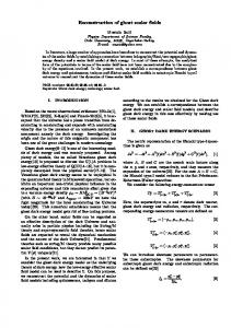
Introduction Visualization is the process of creating visual images from raw data to support human beings with the formation of a mental model and thereby opens the gate for gaining insight. The goal of modern research in visualization is to find visual representations and interaction techniques that maximize human understanding of potentially complex and large amounts of data on a scientific basis. Depending on the application area and data type, modern visualization can be roughly divided into information and scientific visualization [316]. Typically, information visualization deals with abstract and high-dimensional data, whereas scientific visualization is better suited for spatial and low-dimensional data although there exists no clear distinction between these two major fields and plenty of applications combine visual elements from both worlds. The most fundamental parts of a visualization process were formalized by Haber and McNabb [104], who introduced the visualization pipeline as a sequence of basic operations as illustrated in Figure 1.1. Beginning with raw data as input, three major steps are required to obtain the final image: filtering, mapping, and rendering. Filtering involves operations related to selection, preprocessing, and refining the raw data to obtain the actual visualization data. In the mapping stage, this abstract data is transformed into a set of visual representations like geometric primitives to obtain renderable data. In the final step, rendering is performed to obtain the final image by shading and projecting the renderable data onto a rastered screen. The increase of computational power over the last 30 years has been playing a vital role for visualization and science in general. On the one hand, scientific computing deals with the development of algorithms to simulate complex phenomena and generates huge amounts of data with the help of parallel cluster computers. On the other hand, visualization also benefits from this rapid hardware development because it
2 Chapter 1 • Introduction
Raw Data
Filtering
Visualization Data
Mapping
Renderable Data
Rendering
Image Data
Figure 1.1 — The visualization pipeline derived from Haber and McNabb [104].
allows researchers to develop scalable and interactive visualizations, which in turn are valuable and powerful tools for efficient data exploration, sharing experience, and making further developments in the application domain. In particular, in scientific visualization, the computational demands are rather high, because it is often necessary to perform many simple, but costly operations on large amounts of data, for example, to compute derived quantities like gradients or to perform illumination for improved perception of spatial depth. The development of programmable graphics processing units (GPUs) opened new possibilities because their massive and light-weight parallelism naturally facilitates the fast execution of a single task on a large chunk of data. This property soon became attractive in scientific computing because many simulation algorithms follow this principle, too. In this way, both disciplines are fusing together and benefit from each other. The topic of this thesis resides in this emerging field of computational visualization and rendering with a focus on scalar data. Three-dimensional scalar fields are all around us, for example, to describe the varying temperature at each position inside a room. The range of application domains that compute or measure scalar fields is manifold. Well-known examples are data from computer tomography (CT) or magnetic resonance imaging (MRI) providing three-dimensional models of the human body or mechanical parts. In scientific computing, a large class of numerical simulations yield scalar data, for example, the pressure field of a flow simulation, but also more abstract data like the magnitude of the angular momentum of a simulated supernova explosion. Moreover, the appearance of many natural phenomena like clouds, fire, mirages, or fluids is based on the spatially varying material parameters, represented by a scalar field. With global illumination, it is possible to synthesize photorealistic images, for example, in the entertainment or movie industry. Depending on the demands of each of these applications, different visualization and computation techniques are required in terms of the visual properties, accuracy, and performance. The visual properties are defined by a mathematical description of an optical model and is one of the most fundamental elements that drives a threedimensional volume visualization. This thesis introduces three novel optical models for different applications ranging from photorealistic rendering based on physical principles toward more goal-oriented visualizations where a user is more in control of the visual properties. In addition, with increasing data size and the development of massively parallel hardware devices, the computational aspects play an important role
1.1 • Scalar Fields 3 in visualization and scientific computing. However, the characteristics of the hardware are challenging for the development of efficient methods. This thesis introduces three novel algorithms for distributed rendering and computation of scalar fields, specifically developed and optimized for multi-GPU environments. The following sections briefly discuss the general context of this thesis before the research questions and contributions are presented in Sections 1.5 and 1.6, respectively.
1.1
Scalar Fields
A scalar field is a domain in space that stores scalar-valued data at defined positions inside this domain. Formally, a scalar field f is defined as a scalar-valued function that maps each point x = ( x1 , x2 , . . . , xn ) T in the domain D ⊂ R n to a scalar value s ∈ R: f : D → R,
(1.1)
x �→ f ( x) = s.
(1.2)
In the case of a differentiable scalar field, the gradient can be computed and each point x = ( x1 , x2 , . . . , xn ) T in the domain D ⊂ R n is mapped to the gradient vector v ∈ R n of the scalar field f : � x �→ ∇ f ( x) =
∇ f : D → Rn , ∂ f ( x) ∂ f ( x) ∂ f ( x) , ,..., ∂x1 ∂x2 ∂xn
(1.3)
�T
= v.
(1.4)
For the remainder of this thesis, the dimension of all scalar fields is either n = 2 or most often n = 3. Furthermore, in scientific computing and visualization, scalar fields are usually represented as a sampled set of discrete values that are stored in a spatial data structure that can be subdivided into three major classes: gridless, unstructured grid, and structured grid. The data sets that are used throughout this thesis fall into the category of structured grids, in particular, uniform Cartesian grids. For most data sets, it is assumed that the underlying domain is continuous, which requires a method for reconstructing data values at any sample point in the domain. Common reconstruction filters are bilinear (2D) and trilinear (3D) interpolation that linearly weight the four (2D) or eight (3D) neighboring data values depending on their distance to the sample point. In many cases, the achieved quality is sufficient for visualization, which offers efficient computation on graphics hardware and is therefore employed throughout this thesis. However, to obtain results of highest quality, it can be necessary to employ higher-order filters that better approximate an ideal filter [206] at the costs of higher computation times. In addition to the spatial dimensions of a scalar field, time plays also an important role in many applications and is represented as an additional dimension. Formally, an
4 Chapter 1 • Introduction unsteady or time-dependent scalar field f t is defined as: f t : ( D × R ) → R,
(1.5)
( x, t) �→ f t ( x, t) = s.
(1.6)
Similar to the spatial dimensions of a scalar field, the temporal dimension is usually also discretized, most often with equidistant time steps and for each time step, a spatially discretized data set is stored.
1.2
Visualization of Scalar Fields
Due to their wide spreading in many applications, scalar fields play a central role in scientific visualization and computer graphics. This section summarizes how the three generic stages of the visualization pipeline in Figure 1.1 can be interpreted in the context of scalar field visualization.
1.2.1
Filtering
The first stage involves filtering operations that transform the raw scalar field to a welldefined data source for visualization. In the context of scalar fields, filtering is often used as a synonym for the reconstruction of the continuous field from the sampled representation [60, 206], which is closely related to the field of signal processing. Similarly, the estimation of derived quantities like the gradient requires proper filters [28] to avoid artifacts at shading. However, filtering is also important to remedy shortcomings of the data acquisition. For example, medical scanners often exhibit a low signal-to-noise ratio. Therefore, denoising [126] is one of the typical and important operations of this stage. Furthermore, filtering also involves the creation of suitable data structures, for example, multiresolution grids for large data sets [178], but also efficient storage techniques like data compression, such as vector quantization [289] or wavelet-based encodings [226]. Moreover, raw data cannot distinguish between separate parts that have the same scalar value although they might have different origins and meanings. For many applications, it is necessary to segment the raw data into clearly defined regions of interest, for example, by exploiting topological features of the scalar field [334]. Another important filtering technique is clipping [337] that allows one to cut away selected parts of the volume to unveil otherwise hidden details.
1.2.2
Mapping
In the second stage, the still abstract volume data is mapped to renderable primitives together with other relevant attributes like color or opacity. Indirect volume visualization extracts a geometric mesh of an isosurface, for example, with the marching cubes algorithm [194]. The mesh of the isosurface is mapped to triangle primitives together with estimated normals for shading. In contrast, direct volume visualization
1.3 • Computation of Scalar Fields 5 directly samples the voxel data, for example, from a 3D texture and generates a series of fragments [78]. The central element of the mapping stage is the assignment of visual properties. In physically based rendering, material coefficients are determined by real-world phenomena, for example, particle density, albedo, or scattering properties. However, in visualization, the meaning of the scalar data can be manifold and often these data do not exhibit optical properties like emission or absorption coefficients that can be directly used for visualization. Instead a user must decide how this data is mapped to optical properties and this classification is achieved with the transfer function, which is an at least one-dimensional function that maps the range of scalar values to color and opacity. However, multi-dimensional transfer functions [161] can be employed as well, for example, to differentiate between homogeneous areas and sharp transitions by means of the gradient magnitude.
1.2.3
Rendering
The last stage of the visualization pipeline is rendering, that is, the actual image synthesis. Typically, volume rendering is based on an optical model that describes how the classified data is displayed on the screen. Depending on the goals of a visualization, different types of optical models can be employed. For photorealistic image synthesis [96], rendering is usually based on physical light transport in participating media [51] and requires the solution of global illumination. With given material parameters that describe all physical effects of emission, absorption, and scattering, energy transport is simulated accurately with radiometric quantities that are independent of human perception to obtain an objective result solely based on physics. However, there can be several reasons why other optical models can be more suitable. In scientific visualization, the focus is on data exploration and gaining insight instead of realistic appearance. Simplified optical models usually neglect global illumination [116, 211] to accelerate rendering, but also because global illumination is harder to control and it can be difficult to achieve a certain goal. In many cases, these models are also driven by human perception in contrast to realistic rendering. In the extreme case, specialized non-physical models are developed that yield the desired visual properties when visualizing certain volumetric features and that provide easy control for a user. A more recent development is the combination of goal-driven illumination models with the high performance and flexibility of more traditional volume visualization techniques to improve perception of spatial depth and relative size.
1.3
Computation of Scalar Fields
Traditionally, research in many disciplines is based on theory and practical experiments. Over the last decades, scientific computing has emerged as an additional basic field of research that allows scientists to perform virtual experiments by means of computer simulations with the goal to reduce costs or to obtain results from experiments that are impossible to conduct in the real world. The common element of all these virtual
6 Chapter 1 • Introduction experiments is a mathematical formulation of the problem that needs to be solved and since most problems cannot be solved directly, numerical algorithms are usually required to obtain a result. The range of numerical methods for solving the problems in scientific computing cover a wide spectrum, including linear and non-linear equations, optimization problems, initial and boundary value problems, stochastic processes, and many more. A comprehensive overview is beyond the scope of this thesis and the reader is referred to the textbook by Heath [114] that surveys the most fundamental techniques. The focus of the computational part of this thesis is on linear problems where the solution is a scalar field that serves again as input data for a visualization.
1.3.1
Systems of Linear Equations
Systems of linear equations and the computation of their solutions play an important role in many disciplines like engineering, economics, or natural sciences. In particular, many non-linear problems can be approximated with piecewise linearization or decomposed in a true non-linear and linear part, for example, the non-linear advection and the linear pressure projection step in an incompressible Navier-Stokes solver [53]. Formally, a system of linear equations is a set of linear equations with the same set of variables and can be written in matrix form: Ax = b,
(1.7)
where A is a m × n matrix, x is the unknown solution vector with n entries, and b is a vector with m entries. The solution set of a linear system depends on the properties of the matrix as well as on the relationship between the number of equations and the number of unknowns. An overdetermined system has more equations than unknowns, that is, m > n and there often exists no exact solution. However, it is possible to find an approximate solution x¯ so that �b − A x¯ � is minimized under a given vector norm, for example, with the method of linear least squares [127]. In contrast, in an underdetermined system, there are fewer equations than unknowns, that is, m < n and the system has an infinite number of solutions and additional constraints are required to choose one of these solutions. In compressed sensing [70], the solution is assumed to be sparse, which means that only a small number coefficients are allowed to be non-zero and if there exists a unique sparse solution, compressed sensing can find it. Quadratic linear systems that have the same number of equations as number of unknowns with m = n usually have one unique solution. In particular, systems with sparse matrices play an important role for many applications, for example, to solve partial differential equations with the finite element or finite difference method. Typically, iterative algorithms like the preconditioned conjugate gradient method are employed to compute a solution for large systems [280].
1.4 • Graphics Processing Units 7 Independent of the type of linear system, the computational expense for solving systems with billions of unknowns is very high and requires high performance computers like clusters that connect many physical nodes over a fast network link to combine their storage and computing capabilities for parallel processing.
1.3.2
Cluster Computing
Many clusters contain a large number of rather inexpensive nodes, each equipped with its own dedicated memory and with one or several multi-core central processing units (CPUs). Developing algorithms for such systems requires considerable knowledge of the architecture and hardware characteristics to achieve good scalability concerning data size and performance. However, for many problems, it is intrinsically difficult to reach a speedup that is about equal to the number of nodes for a fixed data size (strong scaling) because the communication overhead increases proportionally. Nonetheless, for data-intense problems, it is often sufficient if an algorithm scales well with data size, that is, by adding more nodes, larger problems can be solved in about the same time (weak scaling). The implementation of parallel algorithms usually relies on application programming interfaces (APIs) that handle communication and synchronization of the different tasks. Closely coupled devices like multi-core CPUs can communicate via shared memory, for example, with the open multi-processing (OpenMP) API [246], whereas the communication between the loosely connected nodes is often implemented with the message passing interface (MPI) API [220]. In many cases, data communication is slower than local memory access and much slower than the actual computation on the CPU, which makes it difficult to optimize a parallel algorithm. With the development of fully programmable graphics processing units (GPUs), the gap between bandwidth and calculation speed is widening even further and poses new challenges for developing efficient algorithms. To obtain high performance under such conditions, it is crucial that a maximum amount of concurrency is achieved, for example, by carefully overlapping computation, memory access, and data transfer. Furthermore, many traditional algorithms cannot be mapped easily to this new kind of architecture because of intrinsic dependencies that require serialization.
1.4
Graphics Processing Units
In this section, a brief overview of programmable GPUs is provided because most contributions of this thesis make use of them to accelerate rendering or computation. This section is based on a book chapter on GPU-accelerated visualization [2].
8 Chapter 1 • Introduction
Rasterizer Stage
Vertex Program Optional
Fragment Program
Optional
Tessellation Control Program
Tessellator Stage
Tessellation Evaluation Program
Geometry Program
Transform Feedback
GPU Memory Resources (Textures, Buffer Objects)
Figure 1.2 — Illustration of the simplified graphics pipeline, based on OpenGL 4.2, with the programmable vertex, tessellation control, tessellation evaluation, geometry, and fragment programs.
1.4.1
The Graphics Pipeline
Traditionally, GPUs compute rasterized images from polygonal data in a sequence of simple operations. The simplified graphics pipeline, based on the open graphics library (OpenGL) 4.2 [291], is illustrated in Figure 1.2 and consists of five programmable stages: vertex, tessellation control, tessellation evaluation, geometry, and fragment programs. The polygonal geometry of a scene is the input of the pipeline. In the first stage, all vertex positions undergo affine transformations like translation, rotation, and scaling. The model-view matrix is applied to transform model coordinates into camera space and a custom vertex program operates on each incoming vertex and its associated data. Typical operations of a vertex shader are manipulations of vertex positions, applying per-vertex lighting, or assigning texture coordinates. The transformed and lit vertices are then assembled to geometric primitives like points, lines, or triangles. The optional tessellation control shader transforms input coordinates into a new surface representation and computes the required tessellation level. The output of the control shader determines how the fixed-function tessellator generates new vertices in the following stage. Subsequently, the tessellation evaluation shader computes displacement positions of the incoming vertices and the new vertex data is handed over to the next step in the pipeline. In general, the tessellation shaders are most valuable if the number of vertices changes much, for example, by applying dynamic level-of-detail. In this way, scene geometry can be tremendously augmented without affecting bandwidth requirements or geometry storage. The optional geometry shader has access to all vertices of the incoming primitive and it can emit new vertices, which are assembled into a new set of output primitives. Alternatively, the geometry shader can also discard vertices or entire primitives and
1.4 • Graphics Processing Units 9 provide some sort of culling. Before OpenGL 4, the geometry shader was also used for mesh refinement, but the tessellation shaders now provide a more suitable and dedicated tool for this purpose. Typical applications of the geometry shader are simpler transformations for which the ratio of input and output vertices is not too large, for example, the construction of a sprite from a vertex. The output of this stage can be written optionally to buffer objects in GPU memory with the transform feedback mechanism to resubmit data to the beginning of the pipeline. In the next step of the pipeline, the primitives are clipped against the viewing frustum and back face culling is performed. The remaining geometry is mapped to the viewport and rasterized into a set of fragments. The output of this stage are the positions of the fragments, the corresponding depth values, and the interpolated values of the associated attributes, for example, normals and texture coordinates. The fragment shader performs computations based on the fragment position and its interpolated attributes. However, this position is fixed for each fragment, that is, a fragment shader cannot manipulate attributes of other fragments. The output of the fragment program is the color and the alpha value of each fragment and optionally a modified depth value. Typical applications of the fragment shader include per-pixel lighting, texture mapping, or casting rays through a volumetric data set.
1.4.2
The General Purpose Computing Pipeline
GPUs have been evolving towards flexible and fully programmable computation devices based on massive thread-level parallelism [223, 306]. The addition of programmable stages and high-precision arithmetic to the pipeline encouraged developers to exploit the computational power of graphics hardware for general purpose computing on GPUs (GPGPU). In this context, the GPU is considered as a generic streaming multiprocessor, following the single instruction, multiple data (SIMD) paradigm, which is applicable to a wide range of computational problems and the recent developments have even led to dedicated GPGPU-cluster systems. General purpose computing is also of high interest in the visualization community because many advanced algorithms do not map well to the stages of the shader pipeline. Figure 1.3 illustrates a simplified model of a GPGPU architecture. Similar to a shader in the graphics pipeline, a compute program (or kernel) executes user-written code on the GPU [159]. However, a compute program is not dedicated to a specific operation and it does not require a graphics API, such as DirectX or OpenGL. Instead, the host code triggers a GPU kernel by setting up a thread configuration and by calling the compute program like a regular function. Once the kernel is deployed, the GPU executes the code in parallel with full read and write access to arbitrary locations in GPU memory. Furthermore, input and output data of the kernels can be transferred over the PCIe bus between system memory and GPU resources. Several implementations of this thesis are based on the Compute Unified Device Architecture (CUDA) [244], which implements a GPGPU architecture and allows access
10 Chapter 1 • Introduction CPU Sequential Program Execution GPU Parallel Execution
GPU Parallel Execution
Compute Program 0
Compute Program 1
PCIe
PCIe
GPU Parallel Execution Compute Program n
... PCIe
PCIe
PCIe
GPU Memory Resources (Textures, Buffer Objects)
Figure 1.3 — Illustration of the simplified general purpose computing pipeline with multiple compute programs sequentially called from the CPU.
to the memory and the parallel computational elements of CUDA-capable GPUs with a high-level API and does not require any graphics library. The programming of compute kernels is achieved with an extension to the C/C++ programming language. In contrast to shaders, CUDA kernels have access to arbitrary addresses in GPU memory and still benefit from cached texture reading with hardware-accelerated interpolation. Furthermore, fast shared memory is available for thread cooperation or for the implementation of a user-managed cache. A comprehensive introduction to CUDA programming is provided in the textbooks by Sanders and Kandrot [286] and by Kirk and Hwu [159].
1.5
Research Questions
This section provides an overview of the open challenges that are addressed in this thesis. These research questions are the basis for the subsequent contributions in Section 1.6. Physically based rendering of participating media relies on the radiative transfer equation (RTE) by Chandrasekhar [51], which covers interaction of light due to emission, absorption, and scattering. Recently, a series of publications [46, 101, 131, 301, 310] presented rendering algorithms for more complex media that additionally have a continuously varying index of refraction, for example, for rendering mirages. These papers strongly focus on the efficient computation of curved light rays to account for continuous refraction. Although some techniques solve full global illumination, they are still based on the standard RTE that does not correctly handle conservation of energy in such media. For photorealistic rendering with predictable results, a more accurate description of light transport is required that is rigorously based on physical principles and that does not contain any visually noticeable systematic error.
1.5 • Research Questions 11 In general, visual quality and interactivity play important roles in visualization [147]. In volume rendering, it was shown that illumination has a positive influence on how humans perceive shape and spatial depth [191], which is crucial to gain insight. However, in contrast to photorealistic rendering, users also need to explore data sets interactively, which requires a good balance between visual fidelity and performance. Soft shadows and approximated multiple scattering can help to deduce the spatial arrangement of volumetric features, but full global illumination is too expensive. Therefore, a simplified model is required that can simulate these effects with full interactivity over the transfer function, lighting setup, and camera placement. For time-dependent data sets, it is also necessary that no data-specific precomputation is necessary. Besides illumination, opacity is one of the most fundamental quantities in volume rendering that determines the visibility of volumetric features. In direct volume rendering (DVR), isosurfaces are modeled with Dirac delta distributions in the transfer function, but sometimes it also is necessary to classify narrow, but finite intervals in data space, called interval volumes, which represent generalized isosurfaces of finite thickness. However, depending on the viewpoint and the topology of the scalar field, opacity can vary significantly with standard DVR, which can either lead to high occlusion or high transparency. In both cases, important details remain invisible to the user. Therefore, an extended optical model is required that improves the balance of opacity mapping for interval volumes combined with accurate and efficient reconstruction of the scalar field for high-quality visualizations. In addition to suitable optical models, high rendering performance plays an important role for interactive visualization and is challenging for larger data sets and higher image resolutions. Therefore, distributed and GPU-based rendering can be combined to achieve data and performance scalability. While object-space decompositions scale well with the data size, it is difficult to implement DVR algorithms that require some kind of ray coherence such as volumetric shadows. In contrast, image-space decompositions facilitate the development of such algorithms in cases where data size is not the limiting factor. However, GPUs have only limited memory capabilities and it should be at least possible to efficiently combine all the available GPU memory in the entire cluster domain. At the same time, load imbalances must be avoided when the viewpoint changes to achieve high and constant frame rates. In some cases, the biggest challenge of a visualization is the computation of the underlying data. One such example is the volumetric rendering of astronomical nebulae because observational telescope data is limited to the view from Earth and only two-dimensional. However, the approximate symmetry of many nebulae can be exploited to automatically reconstruct a plausible volumetric model from a single telescope image by iteratively solving a system of linear equations. Nonetheless, the problem is strongly ill-posed and cannot be solved with standard techniques without suffering from artifacts or overly symmetric results. Therefore, a dedicated algorithm is required that accounts for the specific requirements and that can be parallelized
12 Chapter 1 • Introduction on a distributed GPU cluster to achieve data scalability and to reduce computation time. The computational power of multiple GPUs can also be exploited to accelerate standard algorithms for solving well-posed linear systems. Traditionally, Krylov subspace methods are widely used to solve sparse systems of linear equations. Preconditioning of the linear system is often employed to accelerate computation, but the hardware characteristics of GPUs make it difficult to achieve any speedup with common preconditioners, which requires the development of novel approaches that are better suited for these architectures. Another challenge is performance scalability because the problem is strongly limited by bandwidth, which becomes even more problematic with multiple GPUs. Therefore, efficient latency hiding is required by exploiting asynchronous data transfer and computation.
1.6
Contributions and Outline
This section briefly provides the author’s contributions of this thesis to the fields of rendering, scientific visualization, and scientific computing. Figure 1.4 illustrates the organization of the chapters and puts the different topics in perspective. Note that Chapter 2 is not a contribution of this thesis since it only summarizes basic techniques as well as previous work. All subsequent publications were co-authored by the author’s PhD advisor Daniel Weiskopf. Chapter 3 presents a generalization of the well-known radiative transfer equation to heterogeneous participating media that have a spatially varying index of refraction, represented as a continuous scalar field. Basic principles from non-linear Hamiltonian optics are reviewed to introduce a physically based light transport equation to the graphics and visualization community that accounts for curved trajectories and, in particular, for correct conservation of energy by means of an extended definition of radiance. A complete formal derivation of the optical model is presented for full reproducibility of all steps. As a secondary contribution, an extension of the photon mapping algorithm [143] is presented that solves the novel model accurately. It is shown that previously published rendering approaches fail to conserve energy in such complex media. The more general light transport equation also facilitates the accurate rendering of time-dependent light transport, for example, for time-of-flight imaging or for rendering of light echoes. This work was published in a regular journal paper at ACM Transactions on Graphics [1] and is co-authored by Christoph Bergmann, who developed a first GPU implementation of the non-linear photon mapping algorithm as part of his Diplom (MSc) thesis. However, for publication, the implementation was completely redesigned in the Mitsuba framework [132] by the author of this thesis. In Chapter 4, a simplified optical model is introduced for the efficient illumination and interactive visualization of volumetric data sets. In participating media, far-range scattering effects often do not contribute much radiance to the final image due to the
1.6 • Contributions and Outline 13 Computational Visualization of Scalar Fields Chapter 3
Chapter 4
Chapter 5
Chapter 6
Light Transport
Efficient Illumination
Opacity Mapping
Parallel Visualization
Rendering
Visualization
Chapter 7
Chapter 8
Parallel Parallel Reconstruction Preconditioning
Computation
Figure 1.4 — Structural overview of the contributions of this thesis.
exponential attenuation. As a consequence, this chapter presents a novel illumination model that confines multiple scattering into spheres of finite radii around any given sample point. A Monte-Carlo simulation preintegrates light transport for a set of material parameters like anisotropy and extinction. At rendering, a small preintegration table is accessed to efficiently estimate ambient light transport by a simple texture lookup. The presented approach effectively generalizes local shadowing techniques like volumetric ambient occlusion [122]. In particular, the algorithm provides interactive volumetric scattering and soft shadows, with interactive control of the transfer function, anisotropy parameter of the phase function, lighting conditions, and viewpoint. Since preintegration does not depend on the data set or transfer function, the technique is also well suited for the visualization of time-dependent data. The contribution of this chapter was published in a conference paper at IEEE SciVis 2013 [5] and received an Honorable Mention award. Filip Sadlo co-authored this publication and contributed valuable data sets and expertise from computational fluid dynamics and flow visualization. Chapter 5 introduces a novel optical model, based on emission and absorption, for visualizing interval volumes and isosurfaces with scale-invariant opacity. The introduced technique is derived from the visual properties of isosurfaces, which means that opacity does not vary with the viewpoint and that scale has no influence. In standard DVR, opacity is strongly affected by the distance that a ray traverses in the spatial and data domain. With the introduced model, this potentially strong imbalance of opacity is avoided by developing an algorithm that compensates varying scale in both domains. In this way, the visual properties of interval volumes are closer to the visual properties of isosurfaces than of large volumetric regions. It is shown that the novel model for finite interval volumes is also able to visualize true isosurfaces with constant opacity, which effectively generalizes previous approaches [164, 167]. Furthermore, since the quality of the visualization strongly depends on accurate sampling, a novel and efficient method is introduced to analytically reconstruct the scalar field inside a cubic cell of a uniform grid. By assuming trilinear interpolation, a cubic polynomial is locally computed from only four samples in each cell by exploiting the fast texture unit of modern GPUs. In this way, crack-free rendering can be guaranteed in combination with higher frame rates than with previous reconstruction methods [204]. The contribution
14 Chapter 1 • Introduction of this chapter was published in a conference paper at IEEE SciVis 2010 [9]. Hamish Carr co-authored this publication and contributed valuable expertise in writing the paper. In Chapter 6, a distributed volume rendering algorithm is presented based on an imagespace decomposition with dynamic load balancing for GPU-based cluster systems. The chapter presents a bricking approach that offers improved data scalability, which is a weak point of sort first decompositions, especially for GPU-based rendering. Furthermore, a novel caching strategy is described that exploits frame-to-frame coherence to preload data that is close to the current frustum of each render node. Depending on the viewpoint, the computational load can strongly vary between the render nodes. Therefore, a dynamic load balancing algorithm is introduced that reorganizes the image decomposition based on a per-pixel cost estimation. It is also shown that sort first partitioning is preferable to parallelize algorithms that depend on ray coherence such as visibility culling or volumetric shadows. The work of this chapter was published in a regular journal paper at IEEE Transactions on Visualization and Computer Graphics [11] in 2011 and is an extended version of a previous paper, published at the Eurographics Symposium on Parallel Graphics and Visualization 2007 [218]. Both papers are first-authored by Brendan Moloney, who contributed the dynamic sort first partitioning algorithm for rendering and the hybrid partitioning algorithm for volumetric shadows. In the first paper [218], a rather small cluster with only eight render nodes could be employed. The author of this thesis joined the second paper [11] for porting the implementation to a larger cluster with up to 32 nodes, writing Python scripts for automatic testing, conducting all performance evaluations, and writing parts of the related work and result sections. The paper was also co-authored by Torsten Möller, the advisor of Brendan Moloney, who performed proofreading and contributed expertise in writing the paper. Chapter 7 presents an application for visualizing volumetric models of astronomical nebulae. In this case, volume rendering is not only employed for final display of the data but as a means to compute the scalar field to be visualized from a single telescope image. The approximate symmetry of many emission nebulae is exploited to formulate a linear problem with additional constraints to reconstruct a plausible volumetric model, similar to a computed tomography (CT). However, since the problem is strongly ill-posed, the algorithm must be robust against inconsistent input data. The linear problem is then solved with a compressed sensing algorithm that employs repeated forward and backward projections of the volume and image data, respectively, with a distributed multi-GPU algorithm to handle the large data and to accelerate reconstruction. The contribution of this chapter was published in a conference paper at IEEE SciVis 2012 [13]. The paper was first-authored by Stephan Wenger, who adapted an existing compressed sensing algorithm from image processing to the problem of reconstructing astronomical nebulae with additional constraints. The author of this thesis developed the distributed algorithm that decomposes the storage and computation demands over a GPU cluster. Furthermore, he was responsible for creating results and performance measurements as well as writing parts of the sections on related
1.7 • Reused and Copyrighted Material 15 work, distributed architecture, and results. Stefan Guthe initially implemented the projection operations on a single GPU, which was then further developed by the author of this thesis for distributed processing on the GPU cluster. Dirk Lorenz and Andreas Tillmann assisted with their expertise in mathematics, especially in ill-posed problems and regularization. They were also proofreading the formal part of the reconstruction algorithm. Furthermore, Marcus Magnor, the PhD advisor of Stephan Wenger, coauthored the publication, contributing his long-term experience in the reconstruction and visualization of astronomical phenomena. Parts of this chapter were also published in an overview journal paper at IEEE Computing in Science and Engineering [14] in 2012. This paper was further co-authored by Wolfgang Steffen and Nico Koning, who wrote the sections on interactive 3D modeling and space hydrodynamics. The author of this thesis contributed the section on parallel GPU-based visualization, which is based on the parallel rendering algorithm of Chapter 6. While Chapter 7 presents an algorithm for solving an ill-posed linear problem in the field of astronomical visualization, many other applications require the solution of a well-posed system of linear equations. In particular, the Poisson equation plays an important role, for example, to model diffusion processes, but also for mesh and image editing. The discretization of the Poisson problem leads to a large and sparse system of linear equations, which is often solved with the preconditioned conjugate gradient algorithm. In Chapter 8, a novel preconditioning technique for the Poisson problem is introduced that accelerates computation and is well suited for efficient multi-GPU processing. It is shown that performance of traditional preconditioners is strongly lowered by the hardware characteristics of GPUs. The novel preconditioner is a sparse approximate inverse of the matrix and requires only GPU-friendly matrixvector products. Furthermore, a multi-GPU algorithm is presented that builds on asynchronous computation and data transfer to improve performance scalability. The work of this chapter was published in a conference paper at PDP 2010 [4]. Günter Knittel co-authored the paper and provided valuable tips for the GPU implementation. Wolfgang Strasser contributed with proofreading the manuscript. In an application, the presented technique was employed as part of a 2D Navier-Stokes simulation code to solve for the pressure scalar field [3]. The solver was tightly coupled with an integrated flow visualization environment that allows one to interactively change the boundary conditions of the simulation and visualize the result in real-time. The paper was coauthored by Steffen Frey and Filip Sadlo, who contributed tips on the implementation and flow visualization, respectively. Thomas Ertl, the PhD advisor of Steffen Frey, contributed with proofreading the paper.
1.7
Reused and Copyrighted Material
In this thesis, material from the following ACM copyrighted paper is partly reused with kind permission of ACM by following the ACM Author Rights agreement:
16 Chapter 1 • Introduction • [1] M. Ament, C. Bergmann, and D. Weiskopf, Refractive radiative transfer equation, ACM Transactions on Graphics, 33(2): 17:1-17:22, 2014. Furthermore, material from the following IEEE copyrighted papers is partly reused with kind permission of IEEE by following the agreement for Thesis/Dissertation reuse: • [4] © 2010 IEEE. Reprinted, with permission, from M. Ament, G. Knittel, D. Weiskopf, and W. Strasser, A parallel preconditioned conjugate gradient solver for the Poisson problem on a multi-GPU platform, Proceedings of the 18th Euromicro Conference on Parallel, Distributed, and Network-based Processing, pages 583-592, 2010. • [5] © 2013 IEEE. Reprinted, with permission, from M. Ament, F. Sadlo, and D. Weiskopf, Ambient volume scattering, IEEE Transactions on Visualization and Computer Graphics, 19(12): 2936-2945, 2013. • [9] © 2010 IEEE. Reprinted, with permission, from M. Ament, D. Weiskopf, and H. Carr, Direct interval volume visualization, IEEE Transactions on Visualization and Computer Graphics, 16(6): 1505-1514, 2010. • [11] © 2011 IEEE. Reprinted, with permission, from B. Moloney, M. Ament, D. Weiskopf, and T. Möller, Sort first parallel volume rendering, IEEE Transactions on Visualization and Computer Graphics, 17(8): 1164-1177, 2011. • [13] © 2012 IEEE. Reprinted, with permission, from S. Wenger, M. Ament, S. Guthe, D. Lorenz, A. Tillmann, D. Weiskopf, and M. Magnor, Visualization of astronomical nebulae via distributed multi-GPU compressed sensing tomography, IEEE Transactions on Visualization and Computer Graphics, 18(12): 2188-2197, 2012. • [14] © 2012 IEEE. Reprinted, with permission, from S. Wenger, M. Ament, W. Steffen, N. Koning, D. Weiskopf, and M. Magnor. Interactive visualization and simulation of astronomical nebulae, IEEE Computing in Science and Engineering, 14(3): 78-87, 2012. In addition, Figure 2.4 is reused from the following copyrighted paper with kind permission of John Wiley and Sons by following the license agreement for Dissertation/Thesis reuse (license number 3342461059061): • [149] © 2013 The Authors Computer Graphics Forum © 2013 The Eurographics Association and John Wiley & Sons Ltd. D. Jönsson, E. Sundén, A. Ynnerman, and T. Ropinski, A survey of volumetric illumination techniques for interactive volume rendering, Computer Graphics Forum, 33(1): 27-51, 2014.
Part I Visualization of Scalar Fields
17
Chapter
2
Basics of Volume Rendering Volume rendering has been an active field of research in scientific visualization and computer graphics over the last three decades. This chapter presents and summarizes the most important principles and basic techniques that are relevant for volume rendering and the subsequent chapters of this thesis. Consequently, the following presentation is not part of this thesis’ contribution, but serves as an introduction of nomenclature and to discuss previous work. Parts of Section 2.3.2 were published in a book chapter about GPU-accelerated visualization [2] by the author of this thesis. The organization of this chapter follows a bottom-up approach, beginning with fundamental principles of geometrical optics in Section 2.1 that are relevant for the scope of this thesis, especially for subsequent contributions on light transport in continuously refracting media [1]. The interaction of light in participating media under the laws of geometrical optics is a central aspect of this thesis. The mathematical basis for describing light transport is defined by an optical model, which can be either physically based for photorealistic volume rendering or developed by experts to achieve specific visual properties that are beneficial to gain insight in complex scalar fields with scientific volume visualization. Therefore, Section 2.2 presents a brief overview of optical models that are important for this thesis, especially for the contributions on ambient light transfer [5] and opacity of interval volumes [9]. The process of image synthesis requires an algorithm that computes the actual solution of an optical model for final rendering. Traditionally, a large body of research focuses on the development of efficient rendering algorithms, depending on the optical model, data set size, and progress in hardware development. Section 2.3 provides a discussion of basic rendering algorithms that are essential building blocks for most of the contributions of this thesis.
20 Chapter 2 • Basics of Volume Rendering
2.1
Physics of Geometrical Optics
According to the textbook of Kandel et al. [152], visible light is electromagnetic radiation at frequencies approximately in the range of ν ∈ [428, 749] THz, which corresponds to wavelengths in the range of λ ∈ [400, 700] nm in vacuum. However, throughout the entire thesis, the scale of interest is in the range of millimeters up to light years. In this case, according to Born and Wolf [37], the finiteness of the wavelength can be neglected and it is legitimate to consider the limiting case λ → 0 for the propagation of light, which is known as geometrical optics. An important consequence for rendering and visualization is that energy transport can be conducted along light rays, which are straight lines or curves that are collinear with the wave vector. Furthermore, their trajectories are determined by Fermat’s principle, which states that the path taken by a light ray between two points in space is the path that can be traversed the fastest. A direct consequence of Fermat’s principle is that light rays propagate along straight lines in vacuum, but along curves in media that have a spatially varying index of refraction. Under the laws of geometrical optics, energy transport can be described by a linear superposition of discrete wave packets (photons) that can be considered as massless, point-like particles carrying energy Q = hν, where h is Planck’s constant and ν is the photon’s frequency. Another important assumption of geometrical optics is that the total number of the discrete particles is very high to describe light transport. In this case, the statistical distribution of the particles can be treated as a continuum. Moreover, the state of each particle is completely described by its position and momentum, which lends itself to describe their motion and density in phase space.
2.1.1
Phase Space
The concept of phase space has a long history in mathematics and physics [241]. In general, the phase space describes all possible states of a dynamical system, where each point in phase space corresponds to a unique state. In Hamiltonian mechanics, the phase space consists of canonical coordinates pi for position and qi for momentum. In statistical mechanics, large ensembles of systems can be described with a distribution function f ( p1 , ..., p N , q1 , ..., q N , t), which provides the number of points per unit volume in phase space of a system with N degrees of freedom [315]. The phase space of the previously discussed photon particles consists of three dimensions for the spatial location and three dimensions for the momentum. In vacuum, the momentum of each particle is composed of its direction of travel and its magnitude hν/c, where c is the speed of light in vacuum. Since c and h are constants, the magnitude of the momentum only depends on the frequency. Therefore, the canonical coordinates pi and qi can be replaced with:
( p1 , p2 , p3 ) → ( x, y, z),
(2.1)
(q1 , q2 , q3 ) → (φ, μ, ν).
(2.2)
2.1 • Physics of Geometrical Optics 21 The state of a photon at time t is determined by x = ( x, y, z) for its spatial location, (φ, μ) for its direction of propagation, and ν for its frequency, which is proportional to the photon’s energy. In rendering, it is common practice to describe the direction of propagation in spherical coordinates with a radial unit vector ω = (φ, θ, r = 1) and it is convenient to define μ := cos θ for the following sections. Hence, a system of photons can be described with a phase space density distribution function: � � m−3 sr −1 Hz−1 . (2.3) f ( x, ω, ν, t) In general, photons propagate with group velocity v g in a refracting medium. The
rate j at which particles stream through a small surface area dA⊥ perpendicular to the direction of propagation and through a small cone dω per unit time dt is obtained by: � � j( x, ω, ν, t) = v g f ( x, ω, ν, t)
m−2 sr −1 Hz−1 s−1 .
(2.4)
Until now, Eqn. (2.4) only describes a particle flow rate in phase space that is not yet related to radiometric quantities that are discussed next.
2.1.2
Radiometry
Since each particle carries energy Q, the rate at which energy streams through a small surface area dA⊥ and through a small cone dω per unit time dt is obtained by multiplication, which leads to the formulation of transient spectral radiance: � � W m−2 sr −1 Hz−1 . (2.5) Lν,t = L( x, ω, ν, t) = Qj( x, ω, ν, t) = v g hν f ( x, ω, ν, t) The important relationship between radiance and the distribution function in Eqn. (2.5) is discussed in more detail by Arvo [20] or Pomraning [261], for example. In geometrical optics, radiance is one of the most fundamental measures to quantify radiation. Radiance measures the radiant energy dQ per unit solid angle dω, per projected unit area dA⊥ , per unit frequency dν, and per unit time dt. Alternatively, the radiant energy dQ per unit time dt can be substituted with the radiant flux Φ = dQ/dt: � dΦ( x, ω, ν, t) � W m−2 sr −1 Hz−1 . (2.6) L( x, ω, ν, t) = ⊥ dA dω dν Since the speed of light is very high, temporal changes of the flux propagate almost instantaneously on small scales and the explicit time dependency can be neglected, which leads to spectral radiance: � dΦ( x, ω, ν) � W m−2 sr −1 Hz−1 . (2.7) Lν = L( x, ω, ν) = ⊥ dA dω dν Furthermore, in many cases, it is sufficient to focus on monochromatic radiance, which is independent of the frequency as illustrated in Figure 2.1: � dΦ( x, ω) � L = L( x, ω) = W m−2 sr −1 . (2.8) ⊥ dA dω
22 Chapter 2 • Basics of Volume Rendering
dȦ
Ȧ
dAŏ ds
Figure 2.1 — Radiance measures the number of photons per unit time that are streaming through a small surface area dA⊥ and through a small cone dω.
The main reason for using radiance as a fundamental quantity in rendering is that it remains constant along a light ray in vacuum. For a more comprehensive discussion of radiometry, the reader is referred to the two volumes of Glassner’s textbook [90].
2.1.3
Liouville’s Theorem
In addition to the description of radiometric quantities, the distribution function f is a fundamental quantity in statistical mechanics to describe transport phenomena in phase space. Most important, Liouville’s theorem [89, 192] describes the temporal evolution of the distribution function f . In particular, it states that f is constant along any trajectory in phase space: N ∂f df = +∑ dt ∂t i=1 �
�
∂ ( f q˙ i ) ∂ ( f p˙ i ) + ∂qi ∂pi ��
�
= 0,
(2.9)
continuity equation
where the dot denotes the time derivative. It can be observed that Eqn. (2.9) is a continuity equation in phase space with f being the conserved quantity. A full derivation of Eqn. (2.9) is beyond the scope of this thesis and can be found in the textbook by Tolman [315] on statistical mechanics. In the Lagrangian frame, the total derivative d f /dt of Eqn. (2.10) tracks the temporal evolution of both the coordinates and the distribution function, which means that the photon density of an infinitesimally small volume element remains constant as it moves in phase space. In addition, the partial derivatives of Eqn. (2.10) provide also an equivalent formulation of the temporal evolution in the Eulerian frame for a fixed point in phase space.
2.1.4
Transport Theory
In more general systems such as gas and fluid dynamics, collisions between the particles can occur or external forces can act on the particles, which introduces inhomogeneity terms on the right-hand side of Eqn. (2.9). This general description of migration and interaction of particles leads to Boltzmann’s equation and linear transport theory [47, 72].
2.1 • Physics of Geometrical Optics 23 Radiative transfer is based on the same principles and can be considered as a special case of Boltzmann’s transport equation. In participating media, photons can be emitted, absorbed, or scattered [51]. For example, in ionized gases, photons are emitted due to the recombination of electrons or as the result of a transition from an excited state to a lower level. Depending on the degree of ionization, chemical composition, or the difference of energy, photons of different frequencies are emitted. In general, emission acts as a source term χe that adds photons to the system and thereby increases the density distribution f . In contrast, photons can also be absorbed and the photon’s radiant energy is transformed into internal energy of the absorber; hence, absorption acts as a sink term χ a that decreases f . The third form of interaction occurs when photons are scattered by particulate matter. Depending on the size of the scattering particles compared to the wavelength of a photon, different types of scattering are possible [318]. In contrast to emission and absorption, scattering locally acts as a source and sink term χs at the same time. Photons that are out-scattered of their direction of travel locally decrease f , but increase f at the same time as they are in-scattered into another direction. The combination of Liouville’s theorem and the inhomogeneity terms lead to a general light transport equation in phase space by substituting the canonical coordinates according to Eqns. (2.1) and (2.2): df ∂ f ∂ ( f x˙ ) ∂ ( f y˙ ) ∂ ( f z˙ ) ∂ ( f φ˙ ) ∂ ( f μ˙ ) ∂ ( f ν˙ ) = + + + + + + = χ a + χe + χs . (2.10) dt ∂t ∂x ∂y ∂z ∂φ ∂μ ∂ν Although Eqn. (2.10) is already a complete description of light transfer, it is not in a suitable formulation for volume rendering. However, Eqn. (2.10) serves well as a starting point for the subsequent contributions on refractive radiative transfer in Chapter 3.
2.1.5
Hamiltonian Optics
The transport equation of the previous section describes the statistical behavior of photons and how they interact with matter. However, for a more complete formulation, the equations of motion are required that quantitatively describe the changes of the position, the direction of propagation, the frequency, and the velocity of a photon as it streams in a medium. Since refractive media play an important role in this thesis, the following equations also cover the motion of photons in media with a spatially varying index of refraction. Fermat’s principle states that the optical length of the path followed by light between two points in space is an extremum, where the optical length is the physical length multiplied by the index of refraction [42]. In fact, Fermat’s principle is a special case of a variational problem with fixed end points. Moreover, Fermat’s principle has the same form as Hamilton’s principle, which can be exploited to derive the Hamiltonian formulation of geometrical optics. However, a full derivation of the following equations
24 Chapter 2 • Basics of Volume Rendering of motion is beyond the scope of this thesis and the reader is referred to literature on optics [37, 261]: dx ds dω ds dν ds ds dt
= ω, 1 = (∇ x n − (ω · ∇ x n) ω) , n ν ∂n ! =− = 0, c ∂t c = =: v g . n + ν ∂n ∂ν
(2.11) (2.12) (2.13) (2.14)
Eqn. (2.11) describes the change of position along a curved line element ds, which is equivalent to the direction of propagation ω. In continuously refracting media, ω undergoes changes according to the gradient of the index of refraction n = n( x, ν, t) as shown in Eqn. (2.12). In case that the spatially varying index of refraction is a function of time, the frequency of a photon is also affected. However, for the remainder of this thesis, it is assumed that the index of refraction is quasi-stationary, that is, the refractive properties of the medium vary slowly compared to the speed of light or remain even constant, which is a reasonable assumption for rendering purposes; hence, the frequency of a photon can be assumed to be constant along its path as indicated by the exclamation mark in Eqn. (2.13). Furthermore, the group velocity v g of a photon in refractive and dispersive media is given by Eqn. (2.14).
2.1.6
Further Reading
Literature on physics and optics provide a more comprehensive overview of the previously discussed topics. Fundamental principles of geometrical and Hamiltonian optics are described by Born and Wolf [37] and by Buchdahl [42], respectively. For more details on radiometric quantities, interested readers are referred to the literature of Nicodemus et al. [235, 236] and to the two volumes of Glassner’s reference book [90]. Furthermore, the books by Goldstein [91] and Tolman [315] provide a wealth of information about classical and statistical mechanics, respectively. Linear transport theory is discussed in detail in the textbooks by Case and Zweifel [47] and by Duderstadt and Martin [72]. Finally, van de Hulst [318] provides a comprehensive overview of the different types of light scattering with a focus on small particles.
2.2
Optical Models
The previously discussed principles of geometrical optics are the physical basis for the mathematical description of several optical models. Common to all subsequently discussed models is a formulation in terms of radiance. However, depending on the considered types of light interaction, different visual effects can be achieved. The following discussion begins by introducing the characteristics of a participating
2.2 • Optical Models 25 medium and how it interacts with light, which is the basis for the radiative transfer equation (RTE) that is presented right after. Although the RTE is not the most general optical model, it covers the most important effects that are necessary for photorealistic rendering of participating media such as clouds, fog, water, or smoke. Typically, the full RTE is employed in computer graphics, but only in few cases in scientific volume visualization due to the high complexity. In the latter case, it is often necessary to fall back to simplified optical models like single scattering. Compared to the RTE, no global solution of illumination is required and directional shadows can still be achieved. However, volume visualization traditionally builds on the emission–absorption model in combination with a transfer function that maps the scalar value to color and opacity, which facilitates a data driven control of the visual appearance.
2.2.1
Participating Media
Before introducing the different optical models, this section discusses the necessary assumptions about the properties of a participating medium in this dissertation. It is assumed that a participating medium is composed of a large number of microscopic particles that are spaced far apart from each other compared to their size. Furthermore, the particles are not represented individually, but only as a mass density distribution ρ. The following sections briefly discuss the four most important types of interactions between a participating medium and light as illustrated in Figure 2.2. Absorption Following Chandrasekhar [51], true absorption of radiance in such media can be described by the absorption coefficient σa = κ a ρ where κ a is the mass absorption coefficient. Hence, σa describes how much radiance is absorbed per unit length and is commonly employed in volume rendering. The change of radiance along a differential straight line element ds due to extinction can be expressed with the following ordinary differential equation (ODE): dL( x, ω) = −σa ( x) L( x, ω). ds
(2.15)
In general, the absorption coefficient can depend on both the position x and direction ω. However, for the remainder of this thesis, the absorption coefficient is assumed to be isotropic, that is, σa = σa ( x). Out-scattering Similar to absorption, the scattering coefficient σs = κs ρ quantifies the amount of radiance that is scattered per unit length where κs is the mass scattering coefficient. Scattering can reduce and increase radiance along a ray at the same time. Incoming radiance is out-scattered of its current direction of propagation, which acts like a
26 Chapter 2 • Basics of Volume Rendering
(a)
(b)
(c)
(d)
Figure 2.2 — In participating media, radiance decreases along a ray due to (a) absorption or (b) out-scattering. In contrast, radiance increases by (c) in-scattering or (d) emission.
local sink. The following ODE describes the total change of radiance due to outscattering: dL( x, ω) = −σs ( x) L( x, ω). (2.16) ds Similar to the absorption coefficient, the scattering coefficient can depend on both the position x and direction ω, in general. However, for the remainder of this thesis, the scattering coefficient is assumed to be isotropic as well, that is, σs = σs ( x). In-scattering In-scattering employs the same scattering coefficient σs like out-scattering and acts like a local source. However, in-scattering depends on all radiance contributions from all incoming directions and cannot be computed directly. Nonetheless, a ODE for in-scattering can still be obtained: dL( x, ω) = σs ( x) Li ( x, ω), ds
(2.17)
where Li ( x, ω) is the in-scattered radiance, which will be discussed subsequently. Emission Finally, radiance is also increased by emission of photons, for example, as the result of a conversion of heat to radiative energy. The ODE for emission is: dL( x, ω) = σa ( x) Le ( x, ω), ds
(2.18)
where Le ( x, ω) is the emissive radiance. Scattering Phase Function In-scattered radiance Li ( x, ω) describes the amount of radiance that arrives at point x from all possible directions ω and that is scattered into direction ω: Li ( x, ω) =
Ω
P( x, ω , ω) L( x, ω ) dω ,
(2.19)
2.2 • Optical Models 27 where Ω denotes the sphere of all directions and P( x, ω , ω) is the phase function that describes the angular distribution of scattering. In general, the phase function is anisotropic and its properties heavily depend on the size of the scattering particles. In volume rendering, one of the most commonly employed phase functions is the Henyey-Greenstein (HG) phase function [120], which was originally developed to simulate scattering of light by interstellar dust particles. However, several publications in volume rendering showed [48, 149] that the scattering properties of many other participating media can be approximated as well with the HG phase function: PHG ( x, ω , ω) =
�
1 − g ( x )2
�3/2 , 4π 1 + g( x)2 − 2g( x) ω · ω
(2.20)
where ω · ω is the dot product between the incident direction ω and the outgoing direction ω. In this way, the HG phase function does not depend explicitly on the orientation but only on the angle between the two directions. Furthermore, the HG phase function depends on the anisotropy parameter g ∈ [−1, 1] that describes the relative amount of forward and backward scattering. More precisely, g describes the average cosine of the scattered directions. Figure 2.3(a) shows polar plots of the HG phase function with moderate backward scattering g = −0.5, isotropic scattering g = 0.0, and moderate forward scattering g = 0.5. For atmospheric scattering, the model by Rayleigh [266] provides a more accurate approximation assuming particles that are much smaller than the wavelength. In computer graphics, Rayleigh scattering was employed by several authors [40, 103, 125, 239] for the physically based rendering of the Earth’s atmosphere. The Rayleigh phase function is defined as:
2 � 3 � , (2.21) 1 + ω · ω PR ( x, ω , ω) = 16π which is illustrated in Figure 2.3(b). In addition to the phase function, a central aspect of Rayleigh scattering is the scattering coefficient that highly depends on the wavelength and is responsible for the bluish appearance of the sky or reddish sunsets: σs ( x) =
2π 5 d( x)6 3 λ4
�
n ( x )2 − 1 n ( x )2 + 2
�2 ,
(2.22)
where d( x) and n( x) are the diameter and the index of refraction of the particles at position x, respectively. One of the most general approaches to light scattering is provided by the Lorenz-Mie solution [195, 215] to Maxwell’s equations, which describes the scattering of electromagnetic radiation by spheres that have about the same size as the wavelength. Due to its complexity and practical restrictions, Lorenz-Mie scattering is employed infrequently in graphics or visualization. However, Frisvad et al. [83] recently presented an approach
28 Chapter 2 • Basics of Volume Rendering ��Û
��Û
�Û ���Û
���Û
���Û (a)
��Û
�Û ���Û
���Û (b)
��Û
�Û ���Û
���Û (c)
�Û
���Û (d)
Figure 2.3 — Plots of common phase functions over the polar angle θ, which is defined as the angle between the incoming direction ω and the outgoing direction ω. (a) Henyey-Greenstein phase function with varying anisotropy parameter g = −0.5 (red), g = 0.0 (green), and g = 0.5 (blue). (b) Rayleigh phase function. (c) Mie-Hazy phase function. (d) Mie-Murky phase function.
that is more suitable for volume rendering and that can also handle absorbing media. Two common approximations to Lorenz-Mie scattering were presented by Nishita et al. [240] for rendering of murky and hazy atmospheres. The Mie-Hazy phase function approximates scattering by sparse fog and is given by: ⎛ � �8 ⎞ 1 ⎝ 1 9 1 + (ω · ω) ⎠ , (2.23) PMH ( x, ω , ω) = + 4π 2 2 2 which is illustrated in Figure 2.3(c). In contrast, the Mie-Murky phase function is more suitable for dense fog and is defined as: ⎛ � �32 ⎞ 1 ⎝ 1 33 1 + (ω · ω) ⎠, PMM ( x, ω , ω) = + (2.24) 4π 2 2 2 which is plotted in Figure 2.3(d). For a more comprehensive overview of light scattering and phase functions, the reader is referred to the textbook by van de Hulst [318].
2.2.2
Radiative Transfer Equation
The RTE [51] is the de-facto standard model for the physically based rendering of participating media with global illumination [48]. The RTE combines all four of the previously discussed types of interaction of light and the medium. Therefore, the differential form of the RTE describes the combined change of radiance at point x along a differential line element ds due to absorption (Eqn. (2.15)), out-scattering (Eqn. (2.16)), in-scattering (Eqn. (2.17)), and emission (Eqn. (2.18)): dL( x, ω) = − σa ( x) L( x, ω) − σs ( x) L( x, ω) + σa ( x) Le ( x, ω) + σs ( x) Li ( x, ω) . � �� � �� � �� � �� ds absorption
out-scattering
emission
in-scattering
(2.25)
2.2 • Optical Models 29 In Eqn. (2.25), the effects of absorption and out-scattering can be aggregated by introducing the extinction coefficient σt ( x) = σa ( x) + σs ( x): dL( x, ω) = − σt ( x) L( x, ω) + σa ( x) Le ( x, ω) + σs ( x) Li ( x, ω) . � �� � �� � �� ds extinction
emission
(2.26)
in-scattering
Similarly, the effects of emission and in-scattering can be combined: dL( x, ω) = − σt ( x) L( x, ω) + σt ( x) Ls ( x, ω), � �� � �� ds
(2.27)
source
extinction
by introducing the source radiance term: Ls ( x, ω) = (1 − Λ( x)) Le + Λ( x) Li ( x, ω),
(2.28)
where Λ( x) = σs ( x)/σt ( x) is the albedo of the medium that measures if extinction is dominated by absorption (Λ � 0) or scattering (Λ � 1). Rearranging Eqn. (2.27) yields the final differential form of the RTE: dL( x, ω) + σt ( x) L( x, ω) = σt ( x) Ls ( x, ω). ds
(2.29)
It can be observed that Eqn. (2.29) is a linear first-order ordinary differential equation in terms of L( x, ω) with variable coefficients. Following Pomraning [261], the integral form of the RTE along a straight ray can be obtained. For the sake of clarity, the notation for a line integral in three-dimensional space is shortened according to Definition 1 in Appendix A.1: L( x, ω) =
L ( x , ω) T ( x , x) � b b �� b reduced background radiance
+
x
�
xb
T (u, x)σt (u) Ls (u, ω) du . ��
(2.30)
accumulated source radiance
In Eqn. (2.30), xb denotes a point on the boundary of the domain with a given boundary condition Lb ( xb , ω). Furthermore, T ( x0 , x1 ) is the transmittance along a straight ray that connects two points x0 and x1 in space: � x � 1 σt (u) du . (2.31) T ( x0 , x1 ) = exp − x0
The first term on the right-hand side of Eqn. (2.30) is the background radiance Lb ( xb , ω), which is attenuated by the transmittance of Eqn. (2.31). The second term is the accumulated source radiance Ls ( x, ω) including emission and in-scattering. The latter contribution depends on the in-scattered radiance Li ( x, ω) of Eqn. (2.19), which in turn depends on the solution L( x, ω) of the RTE. This recursion leads to an integral of infinite dimension and is computationally very expensive to solve.
30 Chapter 2 • Basics of Volume Rendering There can be several reasons why the RTE is not always the best choice of optical model. First of all, an accurate solution requires a considerable amount of computational resources and interactive performance is hardly possible. Furthermore, in scientific volume visualization, the requirements are somewhat different than in computer graphics, which has led to the development of more goal and data driven models that are derived from the RTE, but usually simplified or specialized to visually solve certain tasks and to gain insight into complex scalar fields. A comprehensive overview of such simplified model is provided by Hege et al. [116] and by Max [211].
2.2.3
Single Scattering
In media where the albedo or the density is low, light tends to scatter just a few times. In this case, it is possible to approximate the RTE with a model that accounts only for a single bounce of light scattering. In principle, single scattering equation has the same form as the RTE: L( x, ω) = Lb ( xb , ω) T ( xb , x) +
x xb
T (u, x)σt (u) Ls,s (u, ω) du.
(2.32)
However, Ls,s ( x, ω) is the source radiance with respect to single scattering: Ls,s ( x, ω) = (1 − Λ( x)) Le + Λ( x) Li,s ( x, ω).
(2.33)
In contrast to the RTE, the in-scattered radiance Li,s ( x, ω) does not depend on the solution L( x, ω): Li,s ( x, ω) =
Ω
P( x, ω , ω)
L ( x , ω ) T ( xb , x) � b b ��
dω .
(2.34)
reduced background radiance
In Eqn. (2.34), the incoming radiance from all directions is obtained from the reduced background radiance and not by recursion as opposed to Eqn. (2.19). In this way, the incoming light from the boundary condition and external light sources is attenuated by the medium, which leads to volumetric shadows in rendered images.
2.2.4
Emission and Absorption
In scientific volume visualization, emission–absorption is the most commonly employed optical model. In contrast to the previous approach, scattering is neglected completely, which is equivalent to σs = 0 and the extinction σt = σa is equivalent to absorption. Then, the traditional volume rendering equation is obtained by: L( x, ω) = Lb ( xb , ω) T ( xb , x) +
x xb
T (u, x)σa (u) Le (u, ω) du.
(2.35)
2.2 • Optical Models 31 Note that the transmittance is now computed by integrating over the absorption coefficient in Eqn. (2.31). In volume visualization, it is often assumed that the background radiance is Lb ( xb , ω) = 0 and that emissive radiance Le (u, ω) = Le (u) is independent of the direction ω. Computationally, a discrete sum of n samples can be substituted for the integral in Eqn. (2.35): L( x, ω) ≈
n
∑ T (ui , x) σ� a (ui ) L��e (ui ) Δu ,
i =1
(2.36)
=:Lq (ui )
where Lq (ui ) is defined as the associated radiance. Similarly, the transmittance is approximated: � x � σt (u) du (2.37) T (ui , x) = exp − ui � � i −1
≈ exp − ∑ σt (u j ) Δu
(2.38)
� � i −1 = ∏ exp −σt (u j ) Δu
(2.39)
� i −1 � = ∏ 1 − α(u j ) ,
(2.40)
j =1
j =1
j =1
where the opacity is defined as:
� � α(u j ) := 1 − exp −σt (u j ) Δu .
(2.41)
Together, Eqns. (2.36) and (2.40) lead to the discrete volume rendering equation: L( x, ω) ≈
n
i −1 �
∑ L q ( ui ) ∏
i =1
1 − α(u j )
� (2.42)
j =1
In scientific visualization, radiance Lq and opacity α are usually controlled by the transfer function. In this case, the scalar field s : R3 → R is sampled at locations ui and the transfer function maps these values to Lq (s(ui )) and α(s(ui )), respectively.
2.2.5
Further Reading
Additional literature on radiative transfer can be found in the textbooks by Chandrasekhar [51] and Pomraning [261]. While those two references provide comprehensive background information about physics and light transport, the papers by Hege et al. [116] and Max [211] focus more on volume rendering and also present simplified models. In the context of global illumination, Arvo [20] also presented a derivation of the RTE based on a simpler variant of the transport equation from Section 2.1.4. In scientific volume visualization, the emission–absorption model is discussed in detail in the textbook by Engel et al. [78].
32 Chapter 2 • Basics of Volume Rendering
2.3
Volume Rendering Techniques
In general, none of the previously discussed optical models can be solved analytically. Therefore, the search for numerical solutions has led to a large number of different rendering techniques. The following section briefly summarizes the most relevant methods in the context of volume rendering based on the RTE in Section 2.3.1 and based on the emission–absorption model in Section 2.3.2.
2.3.1
Global Volume Illumination
Research in global volume illumination deals with the development of algorithms that solve or approximate the RTE. Most rendering techniques originate from developments in physics, especially from radiative heat transfer [166] and astrophysics [51] of the 1950s and 1960s. For a comprehensive overview, the reader is referred to the paper of Mishra and Prasad [216], who presented a survey on these early techniques. Blinn [34] as well as Kajiya and Von Herzen [151] were one of the early pioneers who studied light transport in participating media for computer graphics and visualization. However, the development of low-cost high performance hardware and the demands of entertainment industry opened the gate for this rather young field of research. Following the taxonomy by Cerezo et al. [48], the subsequent discussion classifies rendering methods as analytic, deterministic, or stochastic approaches. Analytic Methods Only few analytic methods exist and all of them require hard constraints to be fulfilled or make strict assumptions. For single scattering, Sun et al. [308] derived an analytical solution, but their method requires homogeneous media and works only with isotropic point light sources. Later, Zhou et al. [358] presented an extension of this approach for inhomogeneous media that can be represented as a sum of Gaussians. For multiple scattering, an analytic solution in form of an infinite series was presented by Narasimhan et al. [231] together with an extended technical report [232]. However, their approach requires a homogeneous medium of infinite size and works only with an isotropic point light source. Deterministic Methods Many early deterministic methods are based on finite elements. In surface-based rendering, Goral et al. [94] assumed perfect diffuse reflection in the scene to simplify the RTE and develop the radiosity equation. By discretizing the scene with a finite mesh and by using piecewise constant basis functions, diffuse light transport can be solved with a system of linear equations. Later, the radiosity method was extended by Rushmeier and Torrance [279] to handle participating media with isotropic scattering by discretizing the volumetric domain into a finite set of zones. Sillion [297] presented a unified framework to compute light transfer between surface and volume patches.
2.3 • Volume Rendering Techniques 33 Furthermore, Sillion reduced the high computational expense by hierarchical clustering of the discrete elements. Bhate and Tokuta [33] extended the zonal method to simulate anisotropic scattering by employing a truncated spherical harmonics expansion instead of constant basis functions. However, for strong anisotropy, storage and computational complexity increases dramatically. The same observation applies to the discrete ordinate method [210], originally developed by Chandrasekhar [51], that discretizes the sphere of all directions with a finite number of bins. The discrete ordinate method usually suffers from numerical diffusion and spurious beams of light due to the limited angular discretization. Recently, Fattal [81] employed light propagation maps to increase the accuracy of the method by avoiding interpolation, which is one of the main reasons for these artifacts. In optically thick media with a high albedo, light tends to scatter multiple times. Under this assumption, Stam [300] proved formally that the angular variation of a light field tends to become smooth and in the limit of an infinite number of scattering events becomes isotropic. As a consequence, Stam motivated an approximation of the angular dependency of the light field with a truncated Taylor series that accounts only for the first two terms with respect to the direction. By substituting this approximation into the RTE, Stam derived a diffusion equation that can be solved on a discretized grid, which leads to a sparse system of linear equations. The diffusion approximation was exploited by several follow-up papers as a building block for further developments. Jensen et al. [145] presented a subsurface scattering model that computes the boundary condition of the diffusion equation for a plane parallel medium with two opposing point light sources at each ray entry point, similar to a dipole. In this way, the expensive computation of multiple scattering can be approximated efficiently with diffusion theory. Zhou et al. [359] exploited the diffusion approximation to efficiently compute multiple scattering on a coarse representation of a participating medium. Afterward, the lighting of the high-frequency details of the residual field is compensated during ray marching. Similar to the diffusion approximation, Szirmay-Kalos et al. [312] employed the first two terms of the spherical harmonic expansion to approximate the directional dependence of the radiance to compute multiple scattering with a three-pass algorithm. In the first step, energy is distributed from the light sources with wave front tracing. In the second step, the initial solution is refined iteratively on a grid and discrete directions. In the last step, radiance is gathered with ray casting. Recently, Zhang and Ma [355] have presented a PDE-based illumination model that facilitates light transport and multiple scattering by means of an advection-diffusion equation. Although scientific volume visualization often relies on the emission–absorption model, it was shown by several user studies [179, 191, 272] that advanced illumination models can be beneficial for the perception of spatial depth and relative size. Therefore, the visualization community started to develop efficient algorithms that also approximate realistic global effects like multiple scattering and soft shadows. A comprehensive
34 Chapter 2 • Basics of Volume Rendering
(a)
(b)
(c)
(d)
Figure 2.4 — Comparison of different illumination models for interactive volume rendering. (a) Local illumination with gradient-based shading [187]. (b) Directional occlusion shading [290]. (c) Light propagation illumination [272]. (d) Spherical harmonic illumination [172]. All four images are taken from the survey by Jönsson et al. [149]. © 2013 The Authors Computer Graphics Forum © 2013 The Eurographics Association and John Wiley & Sons Ltd.
overview of such advanced illumination techniques for interactive volume rendering is provided by Jönsson et al. [149]. A large number of interactive methods is based on light cones. At each sample point, scattering and shadows are approximated within a finite cone that is directed toward a light source. Originally introduced by Kniss et al. [162, 163] with half-angle slicing, the light cone paradigm was further developed by several authors. Directional occlusion shading by Schott et al. [290] assumed a backward peaked phase function to simulate back scattering of a single head light within a cone that is directed toward the observer. Later, this technique was extended to arbitrary light cone directions by Šoltészová et al. [330]. Ropinski et al. [272] employed a light propagation volume to simulate multiple scattering and soft shadows in a cone. In contrast to previous approaches, this method allows one to employ ray casting for final rendering. Schlegel et al. [288] discovered that soft shadows and scattering effects can be efficiently approximated by integrating extinction over a finite volume and not only along a one dimensional ray. Furthermore, the authors accelerated numerical volume integration by using a 3D summed area table. Similar to previous approaches, Schlegel et al. also employ a cone shaped subvolume for integration. However, since the orientation of the summed area table is aligned with the data set, the cone is approximated and sampled with a series of cuboids. To account for lighting from all directions, truncated spherical harmonics expansions are often employed to approximate scalar quantities like radiance or visibility over
2.3 • Volume Rendering Techniques 35 a spherical domain. Ritschel [271] computed visibility in the volume domain with a spherical harmonics representation to simulate low-frequency shadows. Kaplanyan and Dachsbacher [153] presented an algorithm that combines spherical harmonics with light propagation volumes to plausibly simulate indirect light in participating media with interactive performance. Kronander et al. [172] employed a multiresolution data structure in the spatial domain to reduce the overhead for computing and storing the spherical harmonics coefficients of the visibility and the light field. In many cases, it is sufficient to further simplify light transport and account only for ambient light that is partially blocked or absorbed by local occluders in the vicinity of each sample point [277]. Hernell et al. [122] sampled a spherical region of each voxel with a set of rays to compute an ambient occlusion factor to attenuate ambient light. In this way, the degree of local occlusion is directly coupled to the shading of a point, which provides important visual cues for the spatial arrangement of volumetric features. Ropinski et al. [273] employed local histograms for the neighborhood of each voxel to obtain a representation of the ambient region that is independent of the transfer function, which allows one to update the occlusion information with interactive performance. However, expensive preprocessing is required to create and cluster the local histograms. In volumetric ambient occlusion, the spherical sampling of the local neighborhood of each point is rather expensive. However, since the directional information of the occlusion is not taken into account anyway, the computation can be simplified to increase performance. Diaz et al. [68] employed a 3D summed area table to efficiently estimate an occlusion factor by averaging the opacity of the eight adjacent octants of each point. A similar approach was developed by Schlegel et al. [288], who compute a 3D summed area table of the extinction coefficient. However, in contrast to Diaz et al., the authors employ a number of cuboid shells and weight each shell with their distance to the sample point to compute the ambient occlusion factor.
Stochastic Methods Stochastic methods usually rely on some kind of Monte-Carlo integration, that is, samples are taken according to a probability density function to randomly trace rays or particles within the environment. In this way, the points at which the integrand is evaluated are chosen randomly, which is well suited for high-dimensional integrals like the RTE. Originally, the Monte-Carlo method was developed by Metropolis and Ulam [214] in the context of nuclear weapons design. In computer graphics, MonteCarlo integration in form of unbiased path tracing was employed by Kajiya [150] to solve the rendering equation accurately. In contrast to distributed ray tracing [54], path tracing does not branch a tree of rays at each intersection point, but follows only a single path from the camera with a random walk and accumulates over a large number of paths. Later, path tracing was extended to participating media by Rushmeier [278] and by Pattanaik and Mudur [253].
36 Chapter 2 • Basics of Volume Rendering For specular reflections or anisotropic phase functions, path tracing converges slowly and leads to high variance, which manifests in noisy images. Bidirectional path tracing [176, 324] overcomes some of these issues by tracing two separate random walks, one from the light source and one from the camera. These subpaths are then connected deterministically to generate a large number of complete light paths. Later, Lafortune and Willems [177] extended bidirectional path tracing to participating media. In general, bidirectional path tracing is also an unbiased method, which means that the technique does not introduce a systematic error. The so far discussed stochastic methods rely on generating statistically independent random samples to evaluate the integrand. In contrast, Markov Chain Monte-Carlo techniques obtain random samples that are statistically correlated. The unbiased Metropolis light transport algorithm by Veach [325] first generates a complete path with bidirectional path tracing and then begins to mutate the vertices of the path with a given acceptance probability. In this way, nearby paths can be explored more efficiently depending on the mutation strategy, which can be advantageous compared to bidirectional path tracing. Later, Pauly et al. [254] presented Metropolis light transport for participating media with mutations of the scattering direction and the scattering location. A more thorough discussion of Markov Chain Monte-Carlo techniques can be found in the dissertations of Veach [323] and Jakob [133]. A general approach to compute difficult paths is a two-pass algorithm. One subclass of these algorithms builds on the many-light paradigm [63], which is derived from the instant radiosity algorithm by Keller [156]. First, a set of virtual light sources is distributed from the light sources into the scene with a random walk similar to path tracing. At each scattering bounce, a virtual light source is created and stored in a spatial data structure. For rendering, ray tracing can be employed to loop over the virtual light sources and gather their contribution to compute indirect light at each point. The original method by Keller employs point light sources, which leads to singularities and is prone to artifacts. Recent developments avoid these singularities by using spherical [113], ray [243], or beam [242] light sources. The second class of two-pass algorithms builds on the concept of density estimation to compute radiance. For surface-based rendering, Jensen [141] presented photon mapping as a rendering technique that is well suited for caustics. In the first step, virtual flux particles (photons) are traced from the light sources with a random walk and stored in a spatial map at each diffuse bounce. In the second step, ray tracing is used to gather radiance by estimating the flux density at each intersection point. Two years later, the method was further extended to participating media by Jensen and Christensen [143]. For a comprehensive discussion of both techniques, the reader is referred to the textbook of Jensen [142]. In general, photon mapping is not as prone to high-frequency noise as path tracing, if the radius of the density estimation is large. However, the finite radius introduces bias to the result. In the past few years, research in photon mapping focused on the reduction of bias. The original methods [141, 143] employed circular or spherical kernel shapes to estimate
2.3 • Volume Rendering Techniques 37 density at discrete points in space, which requires a high number of particles to converge. For participating media, Jarosz et al. [140] presented a method that estimates radiance for an entire beam by projecting the contributions of nearby particles on the beam, which effectively reduces the number of required photons to reach the same level of quality. Later, Jarosz et al. [138] provided a comprehensive discussion of several point and beam-based density estimators. In principle, photon mapping requires an infinite number of particles to converge to the true solution of the RTE. However, even a reasonably good approximation of illumination can require a high number of photons to obtain a result of high quality, which leads to a high memory footprint of the photon map. Hachisuka et al. [105, 106] developed a multipass approach that progressively decreases the size of the radiance estimator by means of several photon tracing passes. In this way, photon mapping is no longer bounded by the available amount of memory. The concept of progressive refinement was also adapted to photon beams by Jarosz et al. [139]. Recently, Kaplanyan and Dachsbacher [154] have presented an algorithm that adaptively refines the gather radius to balance local bias and noise for faster convergence. In scientific volume visualization, stochastic methods are employed infrequently due to their rather slow convergence. Csébfalvi and Szirmay-Kalos [61] employed Monte-Carlo integration for volume visualization, but the optical model did not involve global light transport and was mainly developed for visualizing data sets that do not fit entirely into memory. Wyman et al. [351] presented an algorithm for precomputing global illumination of isosurfaces with path tracing. Once the precomputation is finished, rendering and changing the isovalue is interactive. However, the technique cannot be extended to volumetric light transfer. Rezk-Salama [268] presented a Monte-Carlo algorithm that approximates volumetric light transport by restricting scattering events to a limited set of isosurfaces. Similarly, Kroes et al. [171] presented a hybrid Monte-Carlo algorithm that samples the bidirectional reflectance distribution function at surface-like structures and the phase function in volumetric regions. However, only single scattering is solved and interactivity heavily relies on progressive refinement. Recently, Jönsson et al. [148] introduced an extension of the photon mapping algorithm [143]. By tracking the history of photon trajectories, a full recomputation of light transport can be avoided when the transfer function is changed, but is still necessary when the light source is moved or when time-dependent data is visualized.
2.3.2
Emission and Absorption
Typically, scientific volume visualization relies on the emission–absorption model because photorealistic appearance is not of the same interest as in computer graphics. A central aspect of volume visualization and the emission–absorption model is that the mapping of the scalar value to optical properties is controlled by a user with a transfer function. In this way, the meaning of the underlying scalar quantity is
38 Chapter 2 • Basics of Volume Rendering completely decoupled from its visual representation, which allows a user to classify scalar data individually and to extract meaningful information from volumetric data. The subsequent section briefly discusses some important design principles for transfer functions in volume rendering. Afterward, basic volume rendering techniques for the emission–absorption model are presented. Following the taxonomy of Kaufman and Mueller [155], the methods are classified as indirect, object-order, or image-order. Transfer Function Design In a panel discussion at the IEEE Visualization Conference in 2000, the design space for transfer functions was roughly partitioned into image-centric and data-centric [258]. In image-centric design, the transfer function is specified by exploring a set of rendered images, for example with design galleries, and by combining their visual properties via a user interface. Jankun-Kelly and Ma [135] employed a graphical user interface based on thumbnails and spreadsheets to explore the parameter space. König and Gröller [165] decomposed classification of volume data into three domains (data range, color, opacity) that can be mapped separately via dedicated user interfaces that offer predefined suggestions with thumbnails of rendered images to quickly design a transfer function. In data-centric design, the transfer function is specified by analyzing the scalar field. Bajaj et al. [23] presented the contour spectrum that provides information about the area or the enclosed volume of an isosurface to assist a user in finding salient isovalues. Pekar et al. [256] employ the integral of the gradient magnitude over an isosurface to measure the strength of intensity transitions between different material types. Kindlmann and Durkin [158] automatically detect salient boundaries in a data set by analyzing the relationship between the scalar value and its first and second directional derivatives along the gradient direction. Kniss et al. [161] presented multidimensional transfer functions that also employ higher-order derivatives of the scalar field to achieve a more flexible classification. Haidacher et al. [109] employed statistical properties to define a transfer function space for distinguishing different materials. Weber et al. [334] presented a topology-based segmentation of the volume with a contour tree where each region can be classified with a separate transfer function. For a more elaborate discussion on transfer functions and their design, the reader is referred to the survey paper by Arens and Domik [18]. Indirect Volume Rendering Indirect volume rendering techniques employ an intermediate structure to visualize the features of a scalar field. Traditionally, isosurfaces are one of the most salient structures of a scalar field and their visualization plays an important role in many applications because they often represent meaningful quantities. The most common approach for extracting isosurfaces by means of a polygonal mesh is the marching cubes algorithm by Lorensen and Cline [194]. The scalar field is processed by an imaginary cube whose eight vertices determine the polygon that is needed to represent the part
2.3 • Volume Rendering Techniques 39 of the isosurface that passes through this cube. Later, the algorithm was extended to marching tetrahedra by Shirley and Tuchman [293] as well as by Payne and Toga [255]. In this way, ambiguities of the marching cubes algorithm with some configurations could be solved. In this thesis, indirect volume rendering does not play a vital role and the reader is referred to additional literature. Livnat [193] discusses several improvements concerning data structures and acceleration techniques for isosurface extraction. Furthermore, Newman and Yi [234] provide a comprehensive survey of marching cubes extensions and optimizations. Object-order Volume Rendering In contrast to the previously discussed methods, object-order techniques do not require an intermediate structure because they directly map data samples from the spatial domain onto the image plane. The volume splatting method [343] employs a 3D reconstruction kernel to compute the image plane footprint of a volume sample. The algorithm iterates through the volume and projects the footprints of all voxels to image space. Mueller and Crawfis [222] presented a traversal order where the compositing sheets are always parallel to the image plane, which eliminates disturbing bleeding and popping artifacts. Furthermore, Zwicker et al. [360] employed elliptical Gaussian kernels to avoid aliasing artifacts or excessive blurring. Later, the technique was optimized for GPU based volume rendering by Chen et al. [52]. For a more detailed discussion on volume splatting, the reader is referred to the book chapter of Crawfis et al. [58]. Another important class of object-order methods relies on the projection of tetrahedra for the rendering of unstructured volume data. The algorithm by Shirley and Tuchman [293] traverses and projects all tetrahedral cells of the data set onto the image plane, which leads to a collection of triangles. When the triangles are sorted according to their distance to the camera, they can be classified, rasterized, and blended by the graphics hardware. Röttger et al. [275] developed the concept of preintegrated transfer functions for the projected tetrahedra algorithm to efficiently render isosurfaces without sampling artifacts. Furthermore, Kraus et al. [169] presented a corrected perspective interpolation for the triangles to avoid disturbing rendering artifacts and the authors also presented a preintegration table with a logarithmic scale for the distance. Silva et al. [298] provide a comprehensive survey of volume rendering techniques for unstructured data. Probably the most popular class of object-order techniques relies on 2D and 3D texture slicing [78]. Early GPU-based approaches relied on 2D textures and bilinear interpolation. In this case, the volumetric data set is stored in three object-aligned stacks of 2D texture slices, one for each major axis. Depending on the viewing direction, one of these stacks is chosen for rendering so that the angle between the slice normal and the viewing ray is minimized. Once the correct stack is determined, the proxy geometry is rendered back-to-front or front-to-back and texture sampling can be implemented in a fragment shader. Although sampling artifacts can be reduced by using multi-texturing and trilinear interpolation [269], flickering still remains when switching between the stacks. Furthermore, valuable graphics memory is wasted because of needing to store
40 Chapter 2 • Basics of Volume Rendering three copies of the same volume data, a problem overcome with 3D texture-based methods. The introduction of hardware support for 3D textures [43, 62] enabled a new class of slicing algorithms. The volume data is stored in a 3D texture representing a uniform grid. View-aligned polygons are rendered for generating fragments and 3D texture coordinates are used for trilinear resampling of data values [78, 173]. Gradients can be either precomputed for each grid point or calculated on-the-fly to provide local illumination [320]. In a similar way, Westermann and Ertl [342] presented diffuse shading of texture-based isosurfaces. To avoid expensive oversampling, preintegration [275] was adopted for texture based rendering by Engel et al. [79] to handle high frequencies in the transfer function [31], occurring when isosurfaces or similar localized features are classified with sharp peaks in the transfer function. The rendering of large data sets was addressed by Weiler et al. [336], who developed a multiresolution approach based on 3D textures to achieve an adaptive level of detail. In numerical simulations, even larger amounts of 4D volume data is generated. Lum et al. [197] employed compression and hardware texturing to render time-varying data sets efficiently. Furthermore, the exploration of volume data is also inhibited by occlusion. Weiskopf et al. [338] presented a method for volume clipping using arbitrary geometries to unveil hidden details in the data set. Depending on the transfer function, significant areas of the volume can be transparent or opaque, leading to many samples that do not contribute to the final image. Li et al. [188] show how empty space skipping and occlusion clipping can be adapted to texture-based volume rendering. Image-order Volume Rendering Image-order techniques solve the volume rendering equation by casting rays from the virtual camera through the volume. Over the past few years, ray casting has become the most popular volume rendering method, especially since GPUs provide the necessary capabilities. However, ray casting has its origin in CPU-based volume rendering beginning with the pioneering work by Kajiya [151], Sabella [282], and Drebin et al. [71]. Furthermore, ray casting was employed for visualizing isosurfaces directly from volume data without extracting a polygonal mesh. In early work, Levoy [187] presented an isosurface visualization approach where thickness of the transition region stays constant throughout the volume by weighting the opacity of a voxel inversely proportional to the magnitude of the local gradient vector. Parker et al. [249, 250] presented a ray tracing method that analytically computes the intersection point of a ray and an isosurface under the assumption of trilinear interpolation. Ray casting was introduced to GPU-based volume rendering by Röttger et al. [274], followed by an alternative implementation by Krüger and Westermann [173]. However, until then, all implementations relied on multiple rendering passes. With the development of more flexible fragment shaders, Stegmaier et al. [303] presented a single-pass GPU implementation of ray casting. The introduction of GPGPU programming languages further simplified implementation and offers high flexibility independent of the
2.3 • Volume Rendering Techniques 41 graphics pipeline. Maršálek et al. [209] presented an optimized implementation for the compute unified device architecture (CUDA) and showed that there is no performance penalty compared to traditional shader implementations. The quality of rendered images depends on the filtering method that is used to reconstruct the discrete scalar field at arbitrary positions [206]. Lee et al. [185] introduced a GPU-accelerated algorithm to interpolate the scalar field between uniform samples with third-order splines by evaluating the polynomial functions arithmetically. The control points of the splines are sampled with tricubic B-spline texture filtering by using the efficient technique from Sigg and Hadwiger [296] with eight trilinear texture fetches. Marchesin and de Verdière [204] reconstructed a cubic polynomial from the eight vertices of each hexahedral cell by assuming trilinear interpolation. The cubic polynomial is then approximated with three linear segments that can be employed for preintegration. The rendering of isosurfaces requires an adequate sampling rate to ensure artifact-free images. Hadwiger et al. [108] employed adaptive sampling and iterative refinement with a secant method on the GPU. Although preintegration also avoids sampling artifacts, opacity is scaled improperly and depends on the data topology. Therefore, Knoll et al. [164] introduced peak finding, which analyzes the transfer function for peaks in a preprocessing step. Similar to preintegration, a lookup table is constructed that stores possible isovalues for a set of data segments. During ray casting, the color and opacity of each detected isosurface can be read directly from the transfer function.
Chapter
3
Refractive Radiative Transfer Equation The previously discussed volume rendering techniques all rely on the RTE or on simplified optical models. However, the RTE does not cover light transport in all types of participating media. This chapter motivates and introduces a more general transfer equation to the graphics community for the physically based rendering of participating media that have a spatially varying index of refraction. Based on the generic transport equation (2.10) of Chapter 2.1.4, a differential and integral form suitable for rendering is presented and discussed. It is shown rigorously that the continuous bending of light rays leads to a non-linear scaling of radiance. To obtain physically correct results, basic radiance is employed—known from discontinuous refraction—to conserve energy in such complex media. Furthermore, the generic model accounts for the reduction in the speed of light due to the index of refraction to render transient effects like the propagation of light echoes. The presented refractive radiative transfer equation (RRTE) is solved by extending photon mapping with transient light transport in a refractive, participating medium. The impact of the presented theory is demonstrated and analyzed with rendered images of media that are dominated by spatially continuous refraction and multiple scattering. Furthermore, with this model, it is possible to render visual effects like the propagation of light echoes or time-of-flight imagery that cannot be produced with previous approaches. Parts of this chapter were published in a regular journal paper in ACM Transactions on Graphics [1].
44 Chapter 3 • Refractive Radiative Transfer Equation
3.1
Introduction
In heterogeneous media, material properties vary spatially due to different physical processes such as advection or diffusion. Hence, in addition to the scattering and absorption coefficient, the index of refraction is also a function of position due to a varying concentration of different materials or due to changing temperatures. In this case, light rays are bent continuously and propagate along curves according to the ray equation of geometric optics. Previous work on continuous refraction in computer graphics [46, 101, 131, 301, 310] convincingly visualized the geometric distortion in such media, but without providing a more generic rendering equation. The main motivation for a refractive volume rendering equation is a mathematical description of light transport independent of a specific algorithm or discretization, such as a piecewise constant approximation with Snell’s law. A major issue of continuous refraction is conservation of energy due to the continuously changing solid angle along a curved ray. Therefore, radiance is no longer a conserved quantity in transparent media and the well-known light transfer equations [51, 150] are no longer valid in this general case. In this chapter, a rigorous theory from optics literature is discussed to close this gap in rendering. In addition to curved light rays, this unified model also guarantees conservation of energy by employing so-called basic radiance, which previous approaches did not account for. Although basic radiance is a known quantity in the graphics community [111, 322] for the rendering of discontinuous refraction based on Snell’s law, its application to participating media with continuous refraction and an extended volume rendering equation has not been studied yet. Well-known real-world phenomena of continuous refraction include mirages and heat shimmerings. The refractive index of many materials depends on the temperature. In a mirage, air of different temperatures causes light rays to bent continuously in the atmosphere [30, 102, 227, 356]. Depending on the direction of the temperature gradient, inferior or superior images of the surrounding objects can be observed. Figure 3.1 shows a superior mirage of an ocean liner due to a thermal inversion layer in the presence of a participating medium. Global illumination effects are combined from continuous refraction and multiple scattering in the clouds. Other important sources of continuous refraction are impure materials due to mass transport or mixture processes. One of the most fundamental transport phenomena in nature is diffusion, which can be observed in gases, liquids, and solids. According to the laws of diffusion, the concentration of a material in steady state is described by a harmonic function; hence, the refractive index also becomes a smooth function in space [17, 307]. In general, refraction is a result of the varying speed of light in different media. In everyday life, it is perceived that light propagates instantaneously, since the speed of light is far beyond the reaction time scale of human perception. Recently, several timeof-flight (TOF) visualizations [326, 327, 329, 348] and applications [160, 229, 328, 347] have attracted attention in the graphics community to exploit the finite speed of light for the analysis of light echoes. The latter is also an active field of research
3.1 • Introduction 45 Render Time: 5:32h
Figure 3.1 — Rendering of a superior mirage on a cloudy day with an extended photon mapping algorithm solving the refractive radiative transfer equation. Due to a thermal inversion layer, light is refracted continuously in the lower atmosphere. The inset shows a magnification of the far-distant ocean liner, which seems to be mirrored in the sky. Global illumination effects due to multiple scattering in the clouds are combined with continuous refraction.
in astronomy [36, 170]. Stars or supernovae can induce strongly varying bursts of radiation that are reflected by dust in the surroundings of an emitter. The primary contribution of this chapter is the introduction of a single transfer equation from optics to the graphics community that is suitable for rendering of participating and continuously refracting media. For the first time in rendering, a unified theory from Hamiltonian physics is discussed that describes global light transport in such complex media. It is shown formally that the continuous bending of light causes radiance to depend on the spatially varying index of refraction, which is crucial for conservation of energy. For rendering, there are two important implications. First, the conserved quantity is basic radiance. Second, a mathematical model for continuous refraction is presented that does not rely on Snell’s law and a piece-wise constant approximation of the spatially varying index of refraction. Comprehensive details of all mathematical transformations are provided in the appendix for full reproducibility. A direct result of
46 Chapter 3 • Refractive Radiative Transfer Equation this generic approach is also a description of transient light transport, which allows one to render TOF imagery and light echoes. The secondary contribution of this chapter is an extension of photon mapping [143] that solves the unified transfer equation. Practical considerations for implementing continuous refraction in a participating medium are discussed using basic radiance and higher-order integration without relying on Snell’s law. For efficient rendering, the density estimation method by Jarosz et al. [140] is extended to non-linear beams with basic radiance. Furthermore, it is shown how transient light transport can be solved efficiently with photon mapping by storing additional information about the TOF in the photon map.
3.2
Related Work
This section covers previous work related to physics of light transport, the rendering of refractive media, and rendering of time-resolved phenomena. Note that previous work on rendering of participating media is already discussed in detail in Chapter 2.3 and is therefore not repeated here.
3.2.1
Physics of Light Transport
The already discussed RTE [51] is probably the best-known optical model for physically based rendering of participating media. However, the RTE does not account for a spatially varying index of refraction. Therefore, this section reviews more general optical models from physical optics that are required to discuss a refractive radiative transfer equation (RRTE) for rendering. Based on measure theory and functional analysis, Preisendorfer [262, 263, 264] derived a general transfer equation that accounts for the finite speed of light and a heterogeneous distribution of the refractive index. Pomraning [261] presented a more physically oriented derivation that accounts additionally for an explicit time-dependency of the index of refraction. Both derivations require considerable knowledge in theoretical physics and mathematics, which makes it hard to follow all steps for non-domain experts. In an effort to make this topic more accessible to the graphics community, a derivation of the more practical approach of Pomraning is provided in Appendix B. However, in contrast to Pomraning [261, pp.144–153], this chapter focuses on a stationary index of refraction and all mathematical transformations are provided including the source and sink terms due to emission, absorption, and scattering. Common to Preisendorfer and Pomraning is the use of basic radiance in the final transfer equation. In subsequent work, several authors [19, 112, 181, 190, 235] showed independently that basic radiance is, in fact, a fundamental conserved quantity, which obeys the laws of geometric optics and thermodynamics. More recently, alternative formulations of a generic transfer equation have raised attention in the optics literature. An overview is provided by Martí-López et al. [208],
3.2 • Related Work 47 who discuss the different assumptions and issues concerning conservation of energy of four recently published formulations [265, 157, 207, 317]. Common to all these approaches is that they do not employ basic radiance, leading to complex expressions in their transfer equations, which makes it hard to find an integral solution suitable for rendering. Furthermore, neither of these approaches relate their work to Preisendorfer, Pomraning, or the other work on basic radiance.
3.2.2
Rendering of Refractive Media
Early techniques were able to approximate heterogeneous distributions of refractive indices by repeated application of Snell’s law to render atmospheric effects like mirages [30, 227]. Discontinuous refraction effects were also achieved with interactive performance on the GPU [64, 65, 245, 349, 350]. However, these approaches optimize for rendering speed, whereas this contribution focuses on an accurate rendering model. Walter et al. [332] have presented a technique to quickly compute paths that connect points inside and outside a medium while obeying Snell’s law. However, this approach is not applicable to curved paths that result from continuous refraction. In general, the bending of light can be simulated with non-linear ray tracing. Early work by Gröller [98] describes a generic approach to non-linear ray tracing for visualizing mathematical and physical systems. Later, Weiskopf et al. [340] developed a GPU-based non-linear ray tracer primarily for relativistic visualization. In media with spatially varying refraction, the geometric bending of light is described by the solution of the ray equation of geometric optics [37]. Stam and Languénou [301] employed the eikonal equation to render heat shimmering in air with non-constant refractive indices. Global illumination of participating and continuously refracting media was addressed by Gutierrez et al. [101], who extended photon mapping with inelastic scattering and curved light paths, for example, for the simulation of atmospheric effects [102]. However, the approach was not aware of a refractive transfer equation and did not employ basic radiance to conserve energy. With the contribution of this chapter, the importance of basic radiance is shown to obtain physically accurate results. Ihrke et al. [131] achieved interactive frame rates with wavefront-tracking based on the eikonal equation. Energy conservation was achieved by obeying the intensity law of geometric optics on a mesh. However, light transport was simplified to single scattering. Sun et al. [310] presented an octree decomposition of the refractive index field for adaptive ray marching to accelerate rendering, but also limited to single scattering. Cao et al. [46] presented an analytical solution of the ray equation of geometric optics by assuming a constant gradient of the index of refraction, but energy conservation was not discussed and illumination did not include participating media. However, their analytical solution is employed to validate the implementation for this special case.
48 Chapter 3 • Refractive Radiative Transfer Equation
3.2.3
Time-aware Rendering
Probably, the most typical application of time-aware rendering in computer graphics is motion blur [54], simulating real cameras with finite exposure times. Cammarano and Jensen [44] extended photon mapping to implement motion-blurred global illumination in scenes with moving objects. Although these methods are aware of time in principle, they do not solve transient light transport, that is, the temporal change of radiance due to the finiteness of the speed of light. The latter is a central aspect of special relativistic visualization [128, 225, 339], but these methods do not solve global illumination. Transient global light transport was briefly discussed by Arvo [20], who added the explicit time dependency and a temporal derivative to the classic rendering equation. Later, Smith et al. [299] presented a computer vision-oriented model in operator form for TOF applications. Recently, Jarabo [136] have demonstrated how transient light transport can be solved with photon mapping and time-dependent density estimation [44] for surface-based rendering. Jarabo et al. [137] presented a framework for transient light transport combined with special relativistic rendering to visualize light aberration, the Doppler effect, or the searchlight effect. However, neither of these approaches accounted for participating or even continuously refracting media. Transient light transport can be exploited to infer hidden geometry [160, 328] as well as its motion [248] or to rapidly acquire reflectance properties of objects from a single viewpoint with a TOF camera [229]. Wu et al. [348] analyzed transient light transport in frequency space for designing a bare sensor imaging system. Time-resolved imaging can also be employed to separate direct light, subsurface scattering, and interreflections in a scene [347]. Furthermore, light echoes in interstellar dust clouds [36, 252, 267] belong to some of the most visually compelling phenomena in nature that cannot be rendered without transient light transport. However, there exists no previous technique that accurately renders TOF or light echo effects in complex media.
3.3
Refractive Radiative Transfer Equation
The starting point to obtain a more general volume rendering equation is Eqn. (2.10) from Chapter 2.1.4: ∂f ∂ ( f x˙ ) ∂ ( f y˙ ) ∂ ( f z˙ ) ∂ ( f φ˙ ) ∂ ( f μ˙ ) ∂ ( f ν˙ ) + + + + + + = χ a + χe + χs . ∂t ∂x ∂y ∂z ∂φ ∂μ ∂ν
(3.1)
In principle, Eqn. (3.1) is already a complete description of global light transport in participating and refracting media. The basic recipe for obtaining a more practical transfer equation based on radiance is to substitute Eqn. (2.8) and Eqns. (2.11)–(2.14). However, this requires a significant amount of transformations and the interested reader is referred to Appendix B for reproducibility. By employing common notations for the absorption coefficient σa = σa ( x, ν, t), scattering coefficient σs = σs ( x, ν, t), and the phase function P(ω , ω), a suitable formulation of
3.4 • Analysis 49 global light transport can be provided, following the results of Preisendorfer [262] and Pomraning [261]. From Eqn. (3.1) and the steps of Appendices B.1–B.6, the differential form of the RRTE is obtained and summarized in the following theorem. Theorem 1. In a refractive and participating medium with an index of refraction n = n( x, ν) that varies continuously with position x and frequency ν, radiative transport is described by:
σ d L˜ = σa L˜ e − σt L˜ + s P(ω , ω) L˜ dω , (3.2) ds 4π Ω where L˜ = L˜ ( x, ω, ν, t) is called basic radiance and L˜ e = L˜ e ( x, ω, ν, t) emissive basic radiance:
L L˜ = 2 . n
(3.3)
The total derivative of basic radiance L˜ along a curved line element ds is: d L˜ dt ∂ L˜ dx ∂ L˜ dω ∂ L˜ . = + · + · ds ds ∂t ds ∂x ds ∂ω
(3.4)
The major advantage of Eqn. (3.2) compared to other possible formulations of light transport [208] is that it employs basic radiance as the conserved quantity. In this way, Eqn. (3.2) also obeys previous work in geometric optics and thermodynamics [19, 112, 181, 190, 235] and it closely resembles the standard RTE [51] for non-refracting media. Therefore, an integral solution can be obtained easily and common Monte-Carlo rendering techniques can be adapted with ease.
3.4
Analysis
In this section, the differences between the RRTE and the standard RTE are discussed in detail. Furthermore, interesting connections to previous rendering algorithms are provided that convincingly simulated refraction of light, albeit in a less general manner. As a consequence, it is shown why the approach of this chapter is indispensable to obtain physically correct results in the general sense.
3.4.1
Basic Radiance
The most noticeable difference between the RRTE and the RTE is the use of a different ˜ instead of L, but since the index of refraction is dimensionless, radiation quantity L, the measurement unit of L˜ is the same as of L. In fact, L˜ is called basic radiance and is a well-known quantity in optics literature [19, 181, 190, 235, 236]. Basic radiance was previously employed in computer graphics by Hanrahan and Krueger [111] and Veach [322] to correctly render caustics when light rays are refracted at material
50 Chapter 3 • Refractive Radiative Transfer Equation
L1 n1
dA
n0 L0 Figure 3.2 — Illustration of light transport in two transparent media with different, but constant, indices of refraction n1 < n0 . At the boundary dA of the two media, a non-symmetric BTDF is evaluated and the observer receives scaled radiance L1 < L0 .
boundaries as shown in Figure 3.2. By exploiting Snell’s law and the conservation of energy, it can be shown that radiance is scaled according to: L1 =
n21 n20
L0 .
(3.5)
An intuitive explanation of this phenomenon is that flux density changes when light enters a medium with another index of refraction. For the example in Figure 3.2, it is assumed that n1 < n0 . The energy from the lower region that passes through the area dA is dispersed into a larger solid angle in the upper region; hence, radiance decreases due to conservation of energy. To account for the change of radiance at such discontinuous material boundaries, Veach [322] employed a non-symmetric BTDF. This technique works well for discontinuous interfaces between two different homogeneous media as in Figure 3.2, where refraction only occurs at discrete locations that coincide with scattering locations. However, this approach is not applicable for continuously refracting media as in the current case. In general, it would not be possible to model continuous bending of light with a non-symmetric phase function. In contrast, the RRTE describes both phenomena with a unified model and thereby generalizes the previously discussed approach to continuous refraction and anisotropic scattering. In fact, it is shown easily that discrete refraction at a boundary layer is approximated with a special case of the RRTE: Δ L˜ d L˜ L˜ − L˜ 0 ≈ = 1 = ds Δs Δs
L1 n21
− Δs
L0 n20 (3.5)
= 0.
(3.6)
Eqn. (3.6) states that basic radiance L˜ remains constant when a ray crosses a material boundary. In addition, Eqn. (3.6) is a special case of the RRTE by setting σa = σs = 0, that is, a transparent medium. In general, the total derivative describes the change of
3.4 • Analysis 51 basic radiance along any differential path element ds, which is, in this case, a straight line element, except at the material boundary. It is noted that true discontinuous refraction can only be approximated with the RRTE, since the gradient of n in Eqn. (2.12) is not defined at the boundary. However, in this case, an evaluation of Snell’s law can be employed. The transition from a continuous index of refraction to a discontinuous interface, which results in Snell’s law, can be proved formally with Stokes’ theorem [37].
3.4.2
Streaming of Basic Radiance
The second major difference between the RRTE and the RTE is the total derivative of basic radiance and radiance, respectively. According to Eqn. (3.4), the total derivative in the RRTE is: dt ∂ L˜ dx dω d L˜ = + · ∇ x L˜ + · ∇ω L˜ . ds ds ��� � ��∂t �ds �� �ds �� total
temporal
directional
(3.7)
angular
The total change of basic radiance along a differential line element ds is composed of temporal, directional, and angular contributions. The directional derivative is known from the RTE, where it describes the change of radiance in a certain direction. In non-refractive media this direction does not change, since rays propagate along straight lines: formally, the gradient of the index of refraction is zero in Eqn. (2.12), in which case the angular term is zero in Eqn. (3.7), too. Furthermore, the RTE assumes that temporal changes of radiance propagate instantaneously, which is equivalent to assuming that the group velocity v g is infinite in Eqn. (2.14). In this case, the temporal derivative in Eqn. (3.7) vanishes and the common RTE is obtained, except for the formulation with basic radiance. Now, it can be seen that the RTE with radiance is only valid in media with a constant index of refraction; however, many participating media that are commonly rendered in computer graphics, like frosted glass, jade, amber, or wax, have varying refractive indices 1 < n < 2 [189], depending on the level of purity or on the temperature of a material. The physical interpretation of Eqn. (3.7) is closely related to the partially coupled Eqns. (2.11)–(2.14). They describe the motion of a massless point-like particle that does not have any extent or explicit orientation. According to Born and Wolf [37] and Ihrke et al. [131], there exists the following important relationship between the eikonal function S and the trajectory of such a particle: � � � dx � dx ! ∇S � ω= = (3.8) ⇒� � ds � = 1. ds �∇S� This means that the directional derivative of Eqn. (3.7) only vanishes if L˜ is constant. In contrast, the angular derivative of Eqn. (3.7) explicitly depends on the refractive properties of the medium. A necessary condition for the angular derivative to not
52 Chapter 3 • Refractive Radiative Transfer Equation vanish is that the second derivative with respect to the path length is non-zero: d dω = ds ds
�
dx ds
�
=
! 1 (∇ x n − (ω · ∇ x n) ω) = 0, n
(3.9)
which is only the case if ∇ x n = 0 and if ω and ∇ x n are not colinear. In non-refracting media with ∇ x n = 0, the angular derivative of Eqn. (3.7) always vanishes and particles propagate along straight lines. The temporal derivative in Eqn. (3.7) accounts for the fact that any change of position or direction of a particle is coupled to its traveling speed in a refractive medium, that is, to Eqn. (2.14). This allows one to reinterpret the total derivative in Eqn. (3.7) as a Lagrangian derivative with respect to time by multiplying both sides of the RRTE with v g = ds/dt and by applying the chain rule: D L˜ d L˜ ds ∂ L˜ dx dω ˜ = + · ∇ x L˜ + · ∇ω L. := Dt ds dt ∂t dt dt
(3.10)
This formulation of light transport is similar to other time-dependent transport phenomena such as advection in fluid dynamics. The Lagrangian frame of reference is often advantageous because many rendering algorithms, especially Monte-Carlo techniques, solve radiative transfer directly in this frame via particle or ray tracing, such as photon mapping or path tracing. A parametrization of the particle trajectories or the light rays with respect to time facilitates the handling of transient radiative transfer; hence, this description is later employed to derive a formal solution of the transient RRTE. In summary, the total derivative in Eqn. (3.7) describes the variation of basic radiance along the potentially curved trajectory of a particle that travels with a spatially varying group velocity due to inhomogeneous refractive indices.
3.4.3
Continuous Refraction
A significant advantage of the RRTE compared to the RTE is the comprehensive description of continuous refraction in terms of geometry and basic radiance. The geometric shape of refracted light rays can be calculated by substituting Eqn. (2.11) into Eqn. (2.12): d2 x
⇔
d ds
�
2
=
1 n
�
∇x n −
ds� dx n = ∇ x n. ds
dn dx ds ds
� (3.11) (3.12)
Eqn. (3.12) is the ray equation of geometric optics [37] and was employed in several previous publications to calculate the bending of light rays for rendering objects with continuous refraction [46, 101, 131, 301, 310]. While the solution of Eqn. (3.12) describes the geometric effects of continuous refraction properly, it does not guarantee
3.5 • Formal Solution 53 E1 dA1
E0 dA0
E1 ΔA1
E0 ΔA0 (a)
(b)
Figure 3.3 — Illustration of the intensity law of geometric optics. (a) The product of irradiance and differential area remains constant along a tube of rays. (b) Discretization of the wavefront area with a quad mesh.
conservation of energy. In principle, the conservation of energy can be assured by obeying the intensity law of geometric optics [37]: E0 dA0 = E1 dA1 ,
(3.13)
where E0 and E1 denote irradiance values at both ends of a narrow tube formed by all rays proceeding from an area element dA0 to dA1 as shown in Figure 3.3(a). The area patches denote the wavefronts of propagating light, which are the solution of the eikonal equation. However, this formulation is not well-suited for an energyconserving transfer equation based on radiance such as the RRTE. As a consequence, many established rendering algorithms like path tracing or photon mapping could not be employed without significant redesign. In fact, to incorporate Eqn. (3.13) into light transport, beam tracing [115, 333] or wavefront tracing [131] with a geometric mesh are mandatory to keep track of the continuously varying area patches as illustrated in Figure 3.3(b). This approach only works well as long as the wavefronts propagate without much hindrance. However, in participating media with multiple scattering, very complex meshes would be necessary, since at each scattering event the energy is distributed radially in all directions according to the phase function.
3.5
Formal Solution
Since the RRTE is similar to the RTE, many principles can be reused to find a formal solution. Therefore, the subsequent discussion focuses only on the most important differences and the reader is referred to Arvo [20] for the common steps. The most relevant difference is that rays propagate along curved rays, which requires the formal solution of Eqn. (3.12). Furthermore, the curved trajectories also affect the required exponential factor to derive a formal solution due to the substitution theorem of integration. The following discussion distinguishes between the non-transient and the transient RRTE, since, in many cases, it is not necessary to account for the explicit time-dependency.
54 Chapter 3 • Refractive Radiative Transfer Equation
3.5.1
Non-transient RRTE
In the non-transient case, the time derivative in Eqn. (3.4) vanishes and the solution does not depend explicitly on time. In the first step, a function x(s) is defined that yields the position on a curved ray depending on the arc length s and x(s) is obtained by formally solving Eqns. (2.11) and (2.12). In Eqn. (3.12), it can be seen that this is equivalent to finding the solution of the ray equation of geometric optics: � � dx d = ∇ x n. (3.14) n ds ds � �� =:v(s)
With the definition of v(s), Eqn. (3.14) is formally integrated, twice: dv = ∇x n ds
⇒
dx v = ds n
⇒
v(s) = v0 + x ( s ) = x0 +
s s0
∇ x n ds
s v(s ) s0
n
ds ,
(3.15) (3.16)
with initial conditions v0 = v(s0 ) and x0 = x(s0 ). In the second step, an exponential factor [20] is required in form of the transmittance, similar to the standard RTE, to find an integral solution. The substitution theorem leads to: � � � � s � dx � 1 � . (3.17) σt ( x(s )) � τ ( x0 , x1 ) = exp − � ds � s0 ds For � straight � rays in the form x(s ) = x0 + s ω with unit vector ω, it is guaranteed that �dx/ds � = 1 in Eqn. (3.17). However, for curved rays, described by Eqn. (3.16), a closed� � form solution of Eqn. (3.15) would be required to compute �dx/ds �. Nonetheless, we can again exploit between the eikonal function and the trajectory of � the relationship � Eqn. (3.8) with �dx/ds � = 1. Following common practice, the basic source term is defined, which describes how much basic radiance is emitted or in-scattered at point x in direction ω:
Λ J˜( x, ω) := (1 − Λ) L˜ e ( x, ω) + 4π �
Ω
L˜ ( x, ωi ) P(ωi , ω) dωi , ��
(3.18)
=: L˜ i ( x,ω)
where Λ = σs /σt is the albedo and L˜ i denotes the in-scattered basic radiance. Similar to the RTE, it can be observed that the RRTE is a linear first-order ordinary differential equation with variable coefficients, but in terms of basic radiance: d L˜ ˜ + σt L˜ = σt J. ds
(3.19)
Similar to Arvo [20], the exponential factor of Eqn. (3.17) is employed to integrate both sides of Eqn. (3.19), but along a curved path from x0 = x(s0 ) to x = x(s). The following integral solution of the non-transient RRTE is obtained:
3.5 • Formal Solution 55 L˜ ( x, ω) = τ ( x0 , x) L˜ ( x0 , ω ( x0 )) +
x x0
τ (u, x)σt (u) J˜(u, ω (u)) du,
(3.20)
by using again the shortened notation of a line integral, according to Definition 1 of Appendix A.1. In Eqn. (3.20), ω (u) yields the direction of propagation at point u on the curved path similar to Eqn. (3.8). Similar to the formal solution of the RTE, the first term on the right-hand side of Eqn. (3.20) is the reduced basic radiance from the boundary condition, whereas the second term represents the contribution along the curved path due to emission, absorption, and scattering in the continuously refracting medium.
3.5.2
Transient RRTE
For the formal solution of the transient RRTE, the arc length parameter s becomes a function of light propagation time and the function x(s(t)) is redefined. Eqn. (2.14) is employed to get an expression for the differential line element in terms of light propagation time ds = v g dt and that is substituted into Eqn. (3.14). Similar to the nontransient case, it is solved for x with initial conditions v0 = v(s(t0 )) and x0 = x(s(t0 )). Furthermore, the transmittance of Eqn. (3.17) is rewritten in terms of light propagation time and the substitution theorem is again employed: � � � � t � dx � ds 1 � τ ( x0 , x1 ) = exp − (3.21) σt ( x(s(t ))) � dt � ds � dt t � � 0t 1 (3.22) = exp − σt ( x(s(t )))v g dt t0
with x0 = x(s(t0 )) and x1 = x(s(t1 )). Compared to the non-transient case, the group velocity v g is added, which is crucial to obtain the subsequent formal solution. The basic source term of Eqn. (3.18) can be reused for the transient equation, except that explicit time-dependency is required in all radiance terms. The RRTE is reformulated in terms of light propagation time and the Lagrangian derivative from Eqn. (3.10) is employed by multiplying both sides of Eqn. (3.19) with v g = ds/dt: D L˜ ˜ + σt v g L˜ = σt v g J. Dt
(3.23)
Similar to the non-transient equation, the following integral solution of the transient RRTE is obtained along a curved path from x0 = x(s(t0 )) to x = x(s(t)) with group velocity v g : L˜ ( x, ω, t) = τ ( x0 , x) L˜ ( x0 , ω ( x0 ), t0 ) +
x x0
τ (u, x)σt (u)v g (u) J˜(u, ω (u), t (u)) du, (3.24)
56 Chapter 3 • Refractive Radiative Transfer Equation where t (u) is a function that yields the time at point u on the curved path. It can be observed that many principles from the non-transient equation can be reused and adapted by accounting for the finite and spatially varying group velocity during ray propagation.
3.6
Rendering
A formal solution of light transport in terms of basic radiance is advantageous for many existing rendering algorithms even if transient effects are not considered. In participating media with spatially varying refractive indices, radiance varies continuously along a curved ray due to refraction, in addition to emission, scattering, and absorption. However, with basic radiance, the different interactions of light with the medium can be discriminated from each other, while still retaining a unified model with conservation of energy. Instead of continuously adapting radiance due to refraction, for example, by redesigning existing algorithms to obey the intensity law of geometric optics in highly scattering media, light transport can be solved in terms of basic radiance and reuse a large collection of established rendering techniques for participating media with only very small adjustments. In the following, details of an extended photon mapping algorithm are provided that is devised to solve the RRTE. Although the RRTE could be solved with path tracing as well, the curved trajectories do not allow one to send shadow rays, since two points in space cannot be connected anymore [101], leading to very slow convergence.
3.6.1
Photon Mapping
Photon mapping is a two-pass rendering algorithm. In the first pass, flux particles are emitted from the light sources and are traced through the scene with a random-walk. At each scattering event, these virtual photons are stored in a spatial data structure. In the second pass, ray marching directly solves the integral form of the transfer equation by gathering radiance with a density estimation of the virtual photons. This observation is exploited and photon mapping is adapted to solve the integral form of the RRTE. Although photon mapping was previously employed to simulate the bending of light in participating media [101], the latter approach did not account for transient effects and was not aware of basic radiance. Especially, the latter is crucial to conserve energy and to obtain physically correct results, which is shown in Section 3.8 with multiple comparisons. In the following, it is assumed that the volumetric distributions σs , σt and the refractive index n of the medium as well as the light source positions are quasi-static compared to the speed of light. Non-transient Photon Tracing In the first pass, virtual photons are emitted from all light sources, similar to standard photon mapping. However, the trajectory of each virtual photon is described by
3.6 • Rendering 57 Eqns. (2.11) and (2.12), which were employed to derive the RRTE. In Section 3.5, a formal solution was obtained in Eqn. (3.16) for the non-transient case. For the curved path x(s), a solution is computed with the fourth-order Runge-Kutta (RK4) method. While a virtual photon propagates without interaction through the refractive, participating medium, energy is conserved. Intuitively, virtual photons do not gather radiance but carry flux, on which the index of refraction has no influence and the stage of photon tracing can be considered as the evolution of a dynamical system with phase space density f that was employed earlier in Section 2.1. The interaction of a photon with the participating medium is solved with a Markov random walk. For heterogeneous media, the inversion method [259] or Woodcock tracking [312] can be employed to compute the free path distance between two interaction events with non-linear photon marching. At an interaction location, the photon is stored in the photon map and Russian roulette [21] is used to decide if a photon is absorbed or scattered. Since the beam radiance estimation method by Jarosz et al. [140] is extended, each photon is assigned a radius and a bounding box hierarchy is created over the photon-discs for efficient rendering. Transient Photon Tracing For the finite speed of light is accounted by solving Eqn. (3.14) numerically in terms of light propagation time with step size Δt and a spatially varying group velocity v g ( x) = c/n( x) in a non-dispersive medium. v(t) and x(t) are solved numerically, similar to the non-transient case, but with step size Δs( x) = v g ( x)Δt that depends on the local group velocity. Since a quasi-static medium is assumed, transient light transport can be simplified. Instead of emitting and tracing photons continuously over time, the spatial distribution of all photons is computed once and only their flux is adapted in each time step of the rendering process. Therefore, the TOF of each photon is stored in the photon map instead of absolute time values. The TOF is obtained by accumulating the time steps Δt from the numerical integration. Furthermore, the N photons cannot carry flux Φ/N anymore as in non-transient photon mapping, since the flux Φ(t) now depends on absolute time. Instead, each photon is emitted with a weight of 1/N and the flux of each photon is reconstructed by multiplying its weight with the dynamically queried flux during rendering. In addition to the TOF, a unique identifier is stored for the light source that emitted the photon. Scattering The main reason why photon mapping is chosen as rendering method is the straightforward handling of single-scattered light. In non-refractive media, the photon map is not required to solve the single scattering contribution, since straight shadow rays can be traced to sample each light source; hence, photons are only stored in the photon map after at least two bounces. However, in continuously refractive media, this is not possible since there is no general solution to finding a curved path connecting two
58 Chapter 3 • Refractive Radiative Transfer Equation arbitrary points in space. By also storing photons after the first bounce, the single scattering contribution can be solved with a radiance estimation from the photon map as well. The drawback of this approach is that the necessary amount of photons to obtain high-quality results increases. In general, scattering of any order is described by the basic source term in Eqn. (3.18), which includes the estimation of basic radiance L˜ i that is in-scattered at point x in direction ω. For consistency, a full derivation of the basic radiance estimator is provided by employing the distribution function f from Section 2.1 and by regarding all dependencies:
Λ L˜ i ( x, ω, ν, t) = L˜ ( x, ωi , ν, t) P(ωi , ω) dωi 4π Ω
Λ = v g hν f P(ωi , ω) dωi 4πn2 Ω
Λ hν = v g σs f P(ωi , ω) dωi 4πn2 Ω σs
=
Λ 2
4πn
Λ
Ω
1 d4 Q P(ωi , ω) dωi σs dx dωi dν dt
(3.26) (3.27) (3.28)
3
1 d Φ P(ωi , ω) dωi 4πn2 Ω σs dx dωi dν
Λ = L( x, ωi , ν, t) P(ωi , ω) dωi 4πn2 Ω 1 =: 2 Li ( x, ωi , ν, t). n
=
(3.25)
(3.29) (3.30) (3.31)
In transformation (3.26), the definition of basic radiance and Eqn. (2.8) are substituted that were used previously in the derivation. Subsequently, it is expanded with σs and it is exploited the fact that a photon carries energy Q = hν and that the distribution function denotes a density d3 /(dx dω dν). By substituting the flux Φ = dQ/dt, the wellknown relationship between scattered flux and radiance in a participating medium [143] can be reproduced. Non-transient Rendering In the second pass, basic radiance is gathered with non-linear ray tracing that iteratively estimates and attenuates basic radiance along the curved ray. Therefore, the beam radiance estimation method by Jarosz et al. [140] is extended with basic radiance and with curved beams in heterogeneous media as shown in Figure 3.4. In the first step, the trajectory of each curved beam is computed with an RK4 solver and the node positions are stored in a list. At the same time, the transmittance of Eqn. (3.17) is computed with the composite Simpson’s rule [22] and these values are stored with the nodes in the list. In the second step, basic radiance is estimated along the curved beam. However, in contrast to the point-wise density estimation method by Jensen and Christensen [143], basic radiance is computed due to in-scattering for the entire curved
3.6 • Rendering 59 beam in Eqn. (3.20): L˜ b ( x, ω) :=
x
=
x0 x x0
τ (u, x)σt (u) L˜ i (u, ω (u)) du
τ (u, x)
σt (u) n ( u )2
Li (u, ω (u)) du,
(3.32) (3.33)
where the in-scattering term of Eqn. (3.31) is substituted. In Eqn. (3.33), it can be seen that the spatially varying non-linear term n(u)−2 is integrated along the curved beam in contrast to the standard radiance computation. The beam basic radiance of Eqn. (3.33) is then approximated by looping over the k photons that contribute to the curved beam according to their radius r j and their distance d j to the beam: L˜ b ( x, ω) ≈
k
σt (u j )
∑ τ (u j , x) n(u )2 K(r j , d j ) ΔΦ j P(ωj , ω (u j )),
j =1
(3.34)
j
where u j is the projected location of the j-th photon onto the closest curve segment and ΔΦ j is the photon’s weight. Following Jarosz et al. [140], the same smoothing function K is employed. The transmittance values τ (u j , x) can be looked up and interpolated from the previously computed list. To obtain the final beam radiance for rendering, the result is transformed back to normal radiance with the local refractive index at location x: Lb ( x, ω) = n2 ( x) · L˜ b ( x, ω). (3.35) It is important to note that n2 ( x) in Eqn. (3.35) does not cancel out with 1/n2 (u j ) in Eqn. (3.34), since these values depend on the positions along the ray. Transient Rendering The extension to transient rendering is straightforward and follows the same steps as in the previous section to obtain the transient basic radiance for a curved beam: L˜ b ( x, ω, t) ≈
k
σt (u j )
∑ τ (u j , x) n(u )2 K(r j , d j ) ΔΦ j (t (u j )) P(ωj , ω (u j )).
j =1
(3.36)
j
The function t (u j ) returns the time at point u j , which is the absolute time t minus the TOF from x to u j . The TOF values are obtained during time integration and are stored together with the nodes in a list. For transient rendering, the time-dependent flux ΔΦ j (t (u j )) that each photon contributes with respect to absolute time t needs to be determined with the photon map. Since the TOF of each photon since emission is stored in the photon map, the absolute time of emission can be reconstructed. Together with the light source identifier, a look-up of the flux in the emission function of the corresponding light source is performed.
60 Chapter 3 • Refractive Radiative Transfer Equation
n0 n(x)
L0
Figure 3.4 — Non-linear beam estimation of basic radiance. The green nodes are obtained by numerical integration. At each node, the transmittance values are computed and stored in a list. Basic radiance is estimated by looping over all nearby photons, shown in red, and by computing their contribution with a smoothing function according to their distance to the beam.
3.6.2
Discussion
The extensions to standard photon mapping allow one to solve the RRTE and to demonstrate the practical consequences of the contributions. With the first extension, basic radiance is employed instead of normal radiance to correctly render refraction in participating media. In addition to the curved geometry of light rays, this approach guarantees conservation of energy even in very complex participating media with continuous refraction, in contrast to the approach by Gutierrez et al. [101] that only accounts for the geometric effects of refraction. The key difference to regular photon mapping is the strong non-linear dependency of the spatially varying squared refractive index in the integral over the curved path. Since the index of refraction depends on the location, the influence of this additional term cannot be compensated easily, for example, with a simple rescaling of the light source fluxes. In Section 3.8, the impact on rendered images is investigated and a quantitative analysis for one example is provided. It can be observed that the rather technical and complex theory from the previous sections pays off, since the algorithmic extension is quite simple and can be included in any existing implementation of photon mapping without redesigning the entire algorithm. With the second extension, the propagation of global illumination can be visualized in a participating, refractive medium with spatially varying speed of light. The rendering pass integrates over time and estimates basic radiance in space and time. Since each photon travels along a different path through the medium and carries different flux, radiance estimation requires a look-up of the flux at the time of emission of each photon. In principle, this could be achieved by continuously emitting photons over time and
3.7 • Implementation 61 storing them in a 4D photon map. In this case, a finite time interval is required to estimate photon density in time as well, which was employed by Cammarano and Jensen [44] to render motion blur with photon mapping or more recently by Jarabo [136] for surface-based transient rendering. However, this additional dimension would raise the number of photons even further, especially if the emission functions of the light sources contain high frequencies. This issue is circumvented by assuming that the medium and the light sources are quasi-static, which allows one to reuse the spatial distribution of the photons for each point in time. In this way, the TOF is employed to reconstruct the emission signal without loss of information.
3.7
Implementation
The non-linear photon mapping algorithm of the previous section was implemented with C++ in the Mitsuba renderer [132]. The extension for continuous refraction is fully integrated into the framework as a custom integrator plugin that is coupled with the existing render methods for surfaces and non-refracting, participating media. A series of novel container types is supported to model complex media with a spatially varying index of refraction. Mainly for validation purposes, a medium with constant index gradient was implemented because there are analytical solutions to compute the curved trajectories from Eqn. (3.14). The two different approaches by Ghatak [88, Chapter 3.4] using exponential functions and by Cao et al. [46] using logarithmic functions were implemented to cross-validate the analytical solutions. For more realistic scenes, a grid-based medium was implemented with heterogeneous distributions of the index of refraction, density, and color, which allows one to model compositions of different materials or concentrations from physically based simulations like Maya® Fluid Effects™ . For numerical integration of Eqn. (3.14), the Euler method and the RK4 method are supported. For media with a solid surface, the existing BRDFs for dielectric and rough dielectric materials were extended to read the spatially varying index of refraction from the internal medium container to evaluate Snell’s law. In this way, refraction can also vary spatially on the surface with consistent contributions of refraction and reflection due to Fresnel’s equation. To increase render performance, the plugin employs the existing parallelization layer of Mitsuba for multi-threaded and parallel ray tracing on a render cluster.
3.8
Results
This section presents results from the parallel implementation on a cluster with 16 compute nodes, each equipped with 2 Intel Xeon X5620 Quad Core CPUs with 2.4 GHz and 24 GB RAM. The physical nodes are interconnected over an InfiniBand network with a bandwidth of 20 GBit/s. Various results are discussed that show the impact of the approach on rendered images in the presence of scattering and refracting media.
62 Chapter 3 • Refractive Radiative Transfer Equation
30 cm cm
10 cm
30
60
Laser
cm
Toward Camera Render Time: 5:06h
(a)
(b)
Figure 3.5 — Bouncing laser beam due to continuous refraction in a glass tank filled with a sugar solution of varying concentration. (a) Long shot photograph of the realworld experiment. (b) Rendering of the virtual experiment from a similar point of view.
In addition, image sequences of propagating light echoes are shown that illustrate the transient behavior of light transport in such media.
3.8.1
Refraction in Participating Media
Mirages are a well-known phenomenon, where continuous refraction plays an important role. Figure 3.1 shows a rendering of a superior image of a far-distant ocean liner with RRTE-based photon mapping. The mirage is caused by a thermal inversion layer in the lower atmosphere. To obtain realistic data for the temperature-dependent index of refraction, the atmospheric model described by Gutierrez et al. [102] was employed. Due to scattering in the clouds and in the fog, global illumination effects are combined from participating and continuously refracting media. The inset shows a magnification of the mirrored ocean liner and the surrounding clouds. In Figure 3.5, a real-world experiment was conducted, similar to Strouse [307] and Ambrosini et al. [17], to study continuous refraction in a participating medium under controlled conditions in the lab and to validate the implementation. The setup consists of a glass tank (60x30x30 cm) with 18 liters (10 cm height) of fresh water intermixed with one droplet of a 2% eosin solution to increase scattering of light. Afterward, 2 kg of sugar cubes were dissolved on the bottom of the tank. By diffusion and gravity, a concentration profile formed naturally over a time span of 24 h with a decreasing sugar concentration from the bottom toward the top. According to Lide [189], the index of refraction of a sugar solution varies between n = 1.33 (0% concentration, fresh water) up to n = 1.49 (80% concentration) at 20 ◦C. Figure 3.5(a) shows a photograph of the real-world experiment. A green 1 mW laser pointer emits a collimated beam of light that enters the tank horizontally and gets continuously refracted in the sugar
3.8 • Results 63
Reflection of Camera
Render Time: 4:34h
(a)
(b)
Reflection of Camera
Render Time: 4:39h
(c)
(d) 1.42 10 cm
n
1.33 60 cm
(e)
Figure 3.6 — (a) Photograph from the front side. The laser beam enters the tank from the right in a height of 3.30 cm. After one bounce on the bottom, the beam leaves the tank horizontally on the left. (b) Rendering of the setup from (a). (c) Photograph from the front side. The laser is lowered to a height of 2.58 cm. After two bounces, the beam leaves the tank on the left. (d) Rendering of the setup from (c). (e) False-color visualization of the index of refraction inside the sugar solution deduced from the real-world experiment.
solution. On the bottom of the tank, the beam gets partially reflected and is again bent downward. Figure 3.5(b) shows a rendering of the corresponding virtual experiment from a similar point of view. For better comparison, the setup is shown from the front side with dimmed lights in Figure 3.6. In the photograph of Figure 3.6(a), the laser enters the tank in a height of 3.30 cm above the table board. After one bounce, the beam leaves the tank on the left again horizontally. The virtual experiment, in Figure 3.6(b), closely reproduces the trajectory of the beam, its reflections on the back side of the tank, and the scattering of light in the fluid. In the photograph of Figure 3.6(c), the
64 Chapter 3 • Refractive Radiative Transfer Equation
(1)
(5)
(9)
n = 1.33 RTE PM Render Time: 2:21h
(a)
(4)
(8)
(12)
Varying n RRTE PM Render Time: 3:16h
(b)
Figure 3.7 — Heterogeneous cocktail with varying sugar concentration along the vertical axis inside a glass (n = 1.48) with three cherries. (a) Rendering with standard photon mapping assuming a spatially constant index of refraction (n = 1.33) inside the fluid. (b) Rendering with RRTE-based photon mapping assuming a linear distribution along the vertical axis from n = 1.42 at the bottom to n = 1.33 at the top of the fluid. The curved photon and ray trajectories are computed analytically.
3.8 • Results 65 (5)
Snell
Snell
Diff. (1),(4)
(2)
(9)
Diff. (5),(8)
(6)
Piecewise Snell
Diff. (2),(4)
(3)
Piecewise Snell
Diff. (6),(8)
(7)
RK 4 (4)
Diff. (3),(4)
Snell
Diff. (9),(12)
(10)
Piecewise Snell Diff. (10),(12) (11)
RK 4 (8)
Diff. (7),(8)
RK 4 (12)
Diff. (11),(12) 49.4 Radiance [Wsr— 1 m—2]
(1)
0 Analytical
Analytical
Analytical
Figure 3.8 — Closeup renderings of Figure 3.7. Areas (1), (5), and (9) show renderings with constant refraction using Snell’s law together with difference images compared to continuous refraction with analytically computed trajectories in Areas (4), (8), and (12), respectively. The renderings in Areas (2), (6), and (10) are computed by approximating continuous refraction with piecewise evaluations of Snell’s law. The difference images with respect to the analytic solution in Areas (4), (8), and (12) show significant discrepancies. By employing the RK4 method in Areas (3), (7), and (11), the solution closely approaches the analytical result.
laser is lowered to a height of 2.58 cm, which causes the beam to bounce twice before it leaves the tank. Figure 3.6(d) shows a rendering of the changed setup, which closely matches the real-world result. The small discrepancies in all rendered images result from slight deviations of the measured concentration profile. In Figure 3.6(e), a falsecolor visualization of the index of refraction is shown that was employed to render the previous results. The index of refraction varies between n = 1.42 (ca. 50% concentration) on the bottom and n = 1.33 (fresh water) in a height of about 4 cm and above. Note that the distribution also varies slightly in the horizontal direction, probably due to an imperfect distribution of the sugar cubes at the beginning of the experiment. As a consequence, the laser beam gets blurred in Figures 3.6(c) and (d) close to the second bounce.
66 Chapter 3 • Refractive Radiative Transfer Equation In Figure 3.7, the experience from the real-world experiment of Figure 3.5 was applied to an example of everyday life. Many beverages and cocktails contain a significant amount of sugar1 and by mixing different fluids, heterogeneous concentration profiles can occur. In Figure 3.7, it is assumed that the drink consists of sugar-free orange juice (n = 1.33) and grenadine syrup with 18.9 g of sugar per ounce2 , which corresponds to a mass concentration of about 66%; hence the index of refraction is approximately n = 1.45. A linear transition is assumed from pure grenadine syrup on the bottom (y = 0) to pure orange juice on the top (y = 1) of the fluid. The spatially varying index of refraction is then computed by n(y) = (1.0 − y) · 1.45 + y · 1.33 along the vertical axis. For such linear profiles, there exist analytical solutions [46, 88] for the computation of the curved photon/ray trajectories that can be used to validate the numerical solver. In Figure 3.7(a), the fluid is rendered with spatially constant refraction n = 1.33 and standard photon mapping. A spot light illuminates the glass creating a caustic that is partially reflected by the facets of the sphere. In Figure 3.7(b), the same scene is rendered, but the linear distribution n(y) is employed together with RRTE-based photon mapping. All other material parameters remain unchanged. Figure 3.8 shows magnifications of the highlighted areas in Figure 3.7. By comparing Areas (1) and (4) together with their difference image, it can be seen that continuous refraction has a noticeable impact on global illumination. The fluid appears to be more transparent in the upper part of the inset and the shape of the cherries as well as the reflections has changed. Area (2) shows an approximation of continuous refraction by repeated evaluation of Snell’s law; however, compared to the analytic solution, significant discrepancies remain visible. In contrast, the RK4 method closely approaches the analytic result in Area (3). Similar observations can be found for Areas (5) to (8). The reflections of the fluid in the different facets of the sphere depend on the type of refraction and the numerical accuracy of the solver. The shape and position of the caustic on the table board are also affected by the curved trajectories of the photons. In the constant case of Area (9), the triangular shaped caustic is not as focused as in the continuous case in Area (12) and the reflected speckles vary in their positions. In Area (10), the piecewise approximation with Snell’s law fails to sufficiently reproduce the shape of the caustic, in contrast to the higher-order solution in Area (11). In Figure 3.9, a variant of the artificial scene used by Jensen and Christensen [143] and by Jarosz et al. [138] was created to demonstrate the influence of basic radiance. The upper sphere is modeled as an ideal glass sphere that does not scatter or absorb any light. However, due to refraction, a volume caustic is generated in the surrounding grayish, non-refracting medium and in the lower unit sphere. In Figure 3.9(a), a homogeneous orange sphere with a constant index of refraction n = 1.3 is rendered with standard photon mapping. In Figure 3.9(b), the Gauss error function is employed to model a diffusion process inside the sphere with a spatially varying index of refraction that 1 2
http://www.sugarstacks.com/beverages.htm http://www.drinksmixer.com/desc102.html
3.8 • Results 67
Render Time: 1:26h Render Time: 2:19h Render Time: 2:18h
(a)
(b)
(c)
Radiance [Wsr— 1 m—2]
4.03
Render Time: 2:19h
0 (d)
(e)
(f)
Figure 3.9 — The upper glass sphere (transparent, but refracting) generates a volume caustic in the lower sphere (scattering, absorbing, and refracting). (a) The lower sphere has a constant index of refraction n = 1.3 and is rendered with standard photon mapping. (b) The index of refraction increases gradually from n = 1.3 to n = 1.5 according to a diffusion profile. Rendering with standard photon mapping and curved photon/ray trajectories using a correct non-symmetric BTDF [322] at the surface transition. However, energy is not conserved inside the sphere. (c) Rendering with standard photon mapping and curved photon/ray trajectories using an incorrect BTDF. Energy is neither conserved on the surface nor inside the sphere. (d) Rendering with RRTE-based photon mapping and correct energy conservation. (e) Difference image of (b) and (d) with false-color mapping. (f) Difference image of (c) and (d) with false-color mapping.
68 Chapter 3 • Refractive Radiative Transfer Equation continuously decreases from n = 1.5 at the center toward n = 1.3 at the surface. Continuous bending deflects photons and light rays toward the center of the sphere, since the gradient of the index of refraction points in this direction, which changes the shape of the caustic on the floor. In this image, standard photon mapping is employed that accounts for the curved trajectories. However, energy is only conserved at the surface by means of a non-symmetric BTDF [322], but not inside the sphere, where too much radiance is gathered. For full comparison, the scene is also rendered with an incorrect BTDF in Figure 3.9(c), which leads to an even higher overestimation of radiance. In Figure 3.9(d), the impact of basic radiance is demonstrated where RRTE-based photon mapping is employed to achieve full conservation of energy and correct estimation of radiance. Figure 3.9(e) shows a false-color difference image of Figures 3.9(b) and (d), which reveals that radiance is also overestimated in the reflection of the orange sphere, as shown in the magnification of the highlighted region. In Figure 3.9(f), the difference image of Figures 3.9(c) and (d) indicates that the error increases further when using an incorrect BTDF. Note that performance is not affected by correct energy conservation. In Figure 3.10, Maya® Fluid Effects™ was employed to simulate the mixing of melted glass (n = 1.48) and jadeite (n = 1.68) by means of thermal convection and diffusion. The spatially varying index of refraction is obtained with a linear model n( x) = Cg ( x) · 1.48 + Cj ( x) · 1.68, where Cg ( x) ∈ [0, 1] is the concentration of glass and Cj ( x) = 1.0 − Cg ( x) the concentration of jadeite, similar to the volume of fluid method for multiphase flow. In Figure 3.10(a), the cup is rendered with the novel approach. First, the visual impact of continuous refraction with respect to material appearance and caustics is shown. Therefore, the cup is again rendered with spatially constant refractive index n = 1.48 in Figure 3.10(b), while all other material parameters remain the same as in Figure 3.10(a). With constant refractive index, the structure of the material and the caustics remains smooth, which does not agree with the heterogeneity of the complex medium, in contrast to the fine-grained details in Figure 3.10(a). However, simulating continuous refraction as shown in Figure 3.10(a) results in an increase in render time from 2:57h to 4:41h. Second, conservation of energy is studied. In Figure 3.10(a), energy is fully conserved by using a non-symmetric BTDF [322] on the surface and RRTE-based photon mapping inside the medium. In Figure 3.10(c), the cup is rendered with non-linear photon/ray trajectories [101] and with a non-symmetric BTDF [322] on the surface, but with incorrect radiance estimation inside the medium. In Figure 3.10(d), the difference image of Figures 3.10(a) and (c) shows where radiance is overestimated solely due to continuous refraction. For completeness, the cup is also rendered with an incorrect BTDF on the surface in Figure 3.10(e). In Figure 3.10(f), the difference image of Figures 3.10(a) and (e) shows that radiance is drastically overestimated since both errors accumulate. In Figure 3.11, radiance is plotted along the dashed scanlines in Figures 3.10(a), (c), and (e) for a quantitative comparison. The plot reveals that an incorrect BTDF is responsible for a large portion of the error, but a significant discrepancy remains when radiance is not estimated correctly inside the medium. Ultimately, the correct handling of energy conservation is computationally not more
3.8 • Results 69
Varying n RRTE PM Correct BTDF Render Time: 4:41h
n = 1.48 RTE PM Correct BTDF Render Time: 2:57h
(a)
(b)
Varying n nl-RTE PM Correct BTDF Render Time: 4:40h
(c)
Diff. (a),(c)
(d)
Varying n nl-RTE PM Incorrect BTDF Render Time: 4:43h
(e)
Radiance [Wsr— 1 m—2]
1.12
Diff. (a),(e)
0
(f)
Figure 3.10 — Decorative cup made of a heterogeneous mix of light crown glass (n = 1.48) and jadeite (n = 1.68). (a) The spatially varying index of refraction is computed from the concentration of both materials at each point inside the cup. Rendering with RRTE-based photon mapping and full energy conservation. Subtle details of the material are visible and micro caustics are produced on the floor as shown in the two close-up views. (b) The comparison with spatially constant refractive index n = 1.48 cannot reproduce these features sufficiently. (c) Rendering with nonlinear photon/ray trajectories but without energy conservation inside the participating medium. However, a correct BTDF is employed on the surface. (d) The difference image of (a) and (c) reveals that radiance is still overestimated inside the cup. (e) The same setup as in (c) but with an incorrect BTDF. (f) Difference image of (a) and (e).
expensive with the novel approach. Figure 3.12 is an example, where temperature affects the index of refraction. A wax candle is placed inside a vase of frosted glass with constant index of refraction n = 1.55. The surface of the candle is modeled with a rough dielectric BRDF using the GGX microfacet distribution by Walter et al. [331]. Figure 3.12(a) is rendered with standard photon mapping, where a constant temperature of 20 ◦C is assumed, which corresponds
70 Chapter 3 • Refractive Radiative Transfer Equation 2.5
Radiance [W sr −1m−2]
2
Fig. 3.9(a) RRTE with correct BTDF Fig. 3.9(c) nl-RTE with correct BTDF Fig. 3.9(e) nl-RTE with incorrect BTDF
1.5
1
0.5
0 −1 −0.5 0 0.5 1 x-co ordinate of dashed scanline in Figures 3.9(a),(c), and (e)
Figure 3.11 — Quantitative analysis of radiance along the dashed scanlines in Figures 3.10(a), (c), and (e).
to an index of refraction of about n = 1.55 and which is visualized in Figure 3.12(c) with false-color mapping. Figure 3.12(b) is rendered with RRTE-based photon mapping, where a spatially varying temperature distribution of the wax is assumed ranging from about 20 ◦C at the bottom up to 90 ◦C close to the flame. The index of refraction varies between n = 1.55 and n = 1.42, respectively, which is visualized in Figure 3.12(e) with the same color map as in Figure 3.12(c). Figure 3.12(d) shows the difference image of Figures 3.12(a) and (b), before tone mapping. The varying index of refraction leads to observable differences. On the surface, close to the flame, the hot wax appears softer compared to the constant case, mainly due to different Fresnel contributions. Furthermore, global light transport inside the candle and the vase is also affected since photons tend to stream more downward and away from the flame according the index gradient. In Figure 3.12(b), the illumination of the wax varies more smoothly compared to the constant case as highlighted by the left arrows. As a consequence, the vase in Figure 3.12(b) receives more light in the lower regions compared to Figure 3.12(a) as denoted by the right arrows, respectively. The rather high rendering times for both candles are due to the microfacet model on the surface, which leads to slower convergence compared to the other results of this chapter.
3.8 • Results 71
n = 1.55 RTE PM Render Time: 15:19h (a)
1.42
n (c)
1.55 0
Radiance [Wsr— 1 m—2] (d)
Varying n RRTE PM Render Time: 21:41h (b)
9.87 1.42
n
1.55
(e)
Figure 3.12 — A wax candle is inside a vase of frosted glass. (a) Rendering with standard photon mapping. The wax has a constant index of refraction n = 1.55 according to the false-color visualization of (c). (b) Rendering with RRTE-based photon mapping. The wax is modeled with a temperature-dependent index of refraction between n = 1.42 and n = 1.55 according to (e). (d) Difference image of (a) and (b).
72 Chapter 3 • Refractive Radiative Transfer Equation
3.8.2
Light Echoes
The image series of Figure 3.13 shows a result of TOF rendering. The XYZ RGB dragon consists of a heterogeneous mix of amber with varying purity. The index of refraction varies in the range n ∈ [1.53, 1.55]. In Figure 3.13(a), the scene is rendered with stationary lighting to provide an overview. The dragon is illuminated by an area light from the top and by a spot light from the left. In Figure 3.13(b), the area light is turned off completely and the dragon is only illuminated by a short burst of light from the spot light. The head of the dragon appears more saturated than his body because light has already scattered more often. In Figure 3.13(c), the light pulse has almost passed the dragon’s body, which now appears also more reddish due to higher orders of scattering. Meanwhile, the light front has reached the dragon’s tail, which appears again more faint. In Figure 3.13(d), the pulse has passed the dragon completely and the remaining saturated light originates only from multiple scattering inside the dragon. Figure 3.14 shows a real-world application of light echo rendering in astronomy. A variable star emits an intense burst of light, which propagates through the surrounding dust and finally reaches the observer. A well-studied example of a real light echo is V838 Monocerotis3 and serves as a prototype for this result. For the volumetric data set, a single time step of a numerical supernova simulation4 is employed assuming a radius of about 1 light year. Following Magnor et al. [201], the anisotropy parameter is set to g = 0.6 and only slight refraction is simulated in the range n ∈ [1.0, 1.01]. The observation time range in Figures 3.14(a)–(f) corresponds to about 18 months of real time. Meanwhile, the visible structures of the nebula vary significantly due to the transient light transport. Although the volumetric model remains constant throughout the entire image sequence, the scene appears to be dynamic due to the changing lighting conditions. For this result, a CUDA-accelerated implementation of the transient photon mapping algorithm was employed, highly optimized for pure voxelized scenes. The render time of each frame was 110 s on a desktop machine with a 3.4 GHz Intel Core i7 processor, 16 GB RAM and an NVIDIA GTX-680 graphics card.
3.9
Discussion
In this chapter, a physically based optical model was introduced to graphics that describes global illumination in continuously refracting and participating media with a generic volume rendering equation. In previous work, the combination of spatially varying refraction and participating media was solved with simplified models that did not guarantee conservation of energy or did not account for global illumination. The RRTE is independent of a specific algorithm or discretization and has a similar form as the well-known RTE. The main difference is the quantity that is conserved: basic radiance instead of radiance. Thereby, conservation of energy in continuously 3 4
http://hubblesite.org/newscenter/archive/releases/2003/10/ http://vis.cs.ucdavis.edu/VisFiles/pages/supernova.php
3.9 • Discussion 73
(a)
(b)
(c)
(d)
Figure 3.13 — Progression of TOF rendering. The XYZ RGB dragon consists of amber of varying purity with an index of refraction n ∈ [1.53, 1.55]. Rendering with transient RRTE-based photon mapping takes 3:30 h for each frame. (a) Overview with stationary lighting. An area light and a spot light illuminate the dragon. (b) The area light is turned off and the spot light emits a short pulse of light from the left that has already passed the dragon’s head and just reached his body. (c) The light front has almost passed the dragon’s body and reached his tail. (d) The light pulse traversed the dragon completely. Only multiple scattered light illuminates the dragon.
refracting media was achieved and previous approaches that are based on Snell’s law were effectively generalized. The derivation of the RRTE involved several mathematical transformations that are crucial for comprehension; however, the essential benefit of this elaborate discussion is a rather simple implementation in practice. In addition, the computational expense, due to energy conservation, does not increase further compared to pure geometric refraction. With the implementation of photon mapping, the impact of the extended theory on the correctness of rendered images was demonstrated. It was shown that conservation of energy is important in practice as well and that its influence on renderings cannot be neglected, if high accuracy and physical correctness are required. To obtain authentic results, it is crucial that the input data is sufficiently accurate. As a simple example, a real-world experiment was presented in Figure 3.5 and Figure 3.6 to measure the distribution of the refractive index in a heterogeneous sugar solution. However, for more complex media, advanced techniques must be
74 Chapter 3 • Refractive Radiative Transfer Equation
(a)
(b)
(c)
(d)
(e)
(f)
Figure 3.14 — Progression of light echo rendering. (a) The variable star emits a strong burst of radiation. (b) With increasing observation time, light propagates through the medium. (c) Direct light of the star reduces to normal intensity. (d–f) Indirect light continues to propagate, reaches the outer regions, and fades out.
3.9 • Discussion 75 employed to acquire their refractive properties, similar to the scattering properties of participating media [230]. In optics literature, several alternative formulations of light transport without basic radiance were discussed by Martí-López et al. [208] and many of them fail to obey the laws of geometric optics, such as the inverse square law [37]. A noticeable exception is the approach by Martí-López et al. [207], who introduced an explicit term for the divergence of rays that acts as an artificial attenuation or amplification coefficient in their transfer equation to account for the continuously varying solid angle and to achieve conservation of energy. In contrast, the RRTE does not require such an explicit handling of the diverging ray geometry, because basic radiance already accounts for the varying flux density in continuously refracting media and thereby simplifies conservation of energy. However, an interesting direction for future work is to formally investigate the equivalence of both formulations and in case of discrepancies to study the impact on rendering. The current implementation is limited to non-dispersive media, since it does not account for a frequency-dependent index of refraction. However, this is not a limitation of the model, but just of the current implementation. If scattering remains elastic, a discretization of the spectrum could be employed to render independent images for each frequency, since there is no explicit dependency of the frequency present in the RRTE. For practical rendering, the current implementation is mainly limited by the high number of photons that are necessary to estimate direct light. However, further research is required to connect curved light paths with curved eye paths in a continuously refracting medium. A promising approach is the line space gathering method by Sun et al. [309]. Although this technique is currently limited to straight lines, a generalization to curved paths might be possible, for example, with piecewise linear segments. Further algorithmic improvements could be achieved, for example, with progressive photon mapping techniques [105, 106] to improve quality with less memory consumption.
Chapter
4
Ambient Volume Scattering The previous chapter introduced a unified model for light transport for accurate rendering of continuously refracting, participating media. However, solving the RRTE requires significant computational resources, even in non-refracting media, due to multiple scattering, which is infeasible for interactive applications. Therefore, this chapter introduces a simplified optical model derived from the RTE for the interactive rendering and visualization of volumetric data sets. Ambient volume scattering is presented as a preintegration method for scattering on mesoscopic scales in direct volume rendering. Far-range scattering effects often provide negligible contributions to a given location due to the exponential attenuation with increasing distance. This motivates the following approach to preintegrating multiple scattering within a finite spherical region around any given sample point. To this end, full light transport is solved with a Monte-Carlo simulation within a set of spherical regions, where each region may have different material parameters regarding anisotropy and extinction. This precomputation is independent of the data set and the transfer function, and results in a small preintegration table. During rendering, the look-up table is accessed for each ray sample point with respect to the viewing direction, phase function, and material properties in the spherical neighborhood of the sample. Rendering is efficient and versatile because it readily fits in existing ray marching algorithms. It provides interactive volumetric scattering, with interactive control of the transfer function, phase function, lighting conditions, and viewpoint. Parts of this chapter were published in a conference paper at IEEE SciVis 2013 [5] and received an Honorable Mention award. Furthermore, volume renderings with ambient volume scattering won the Computer Graphics Forum 2014 Cover Image Contest [7] and were printed on the front cover of Informatik Spektrum [6].
78 Chapter 4 • Ambient Volume Scattering
4.1
Introduction
Direct volume rendering often relies on the optical model of emission and absorption, which was discussed in Section 2.2.4. However, spatial perception of shape can be difficult, since variation of luminance and shadows are missing, which provide important visual cues for spatial depth under natural lighting. The recent study by Lindemann and Ropinski [191] revealed that shadow-based volume rendering techniques are superior compared to local illumination to determine the relative size of volumetric features. A common alternative to directional shadows is volumetric ambient occlusion that samples the spherical neighborhood of each point to find occluders that attenuate ambient light creating local soft shadows. In this way, concavities appear darker than unoccluded regions. However, the study by Langer and Bülthoff [179] showed that human perception is not solely based on the “dark-means-deep model”. In particular, complex interreflections influence the perception of shape under different lighting conditions. The goal of this chapter is to develop an illumination model that accounts for these aspects. It is shown how directional soft shadows can be combined with indirect lighting from multiple scattering. Ambient volume scattering is computed based on physical light transport within a finite spherical region around each point, similar to ambient occlusion. Many local illumination models [260] rely on normal vectors, which are usually derived from the gradients. However, in homogeneous subvolumes or in areas with low signalto-noise ratio, the direction of the gradient is not numerically stable and shading is susceptible to artifacts. A common alternative is a single scattering illumination model, as shown in Section 2.2.3, based on shadow rays and a phase function. The drawback of that approach is that only a small fraction of light interacts with the medium, which can lead to strong darkening and hard shadows. The latter issues can be avoided with ambient occlusion techniques that integrate extinction over a small spherical neighborhood [68, 122, 273, 277, 304] or a directional cone [290] around each point to compute a local occlusion factor for shading of ambient light. More complex interreflections of light lead to a more natural illumination, but the computation of multiple scattering requires the integration of high-dimensional light transport in the vicinity of each point. Stochastic Monte-Carlo integration is well-suited to solve radiative transfer in participating media [48]. However, to obtain noise-free results, high sampling rates are required, which is computationally too expensive for interactive volume visualization. Nonetheless, high sampling rates are also a wellknown issue in the context of the classic emission–absorption model, especially, if the transfer function contains high frequencies like sharp peaks to visualize isosurfaces. An established technique to accelerate rendering is the preintegration of the transfer function [79, 275] by means of a look-up table. Adapting preintegration to volumetric scattering is, however, not straightforward because scattering requires the solution of global illumination. For inhomogeneous data sets, the dimension of any preintegration technique exceeds practical limits in
4.1 • Introduction 79
(a)
(b)
(c)
(d)
Figure 4.1 — Volume renderings of a supernova simulation with different optical models. (a) Standard emission–absorption model (64 fps). (b) Volumetric ambient occlusion (27 fps). (c) Single scattering model with a point light source in the center of the supernova (31 fps). (d) Ambient volume scattering model with the same point light source (20 fps).
80 Chapter 4 • Ambient Volume Scattering terms of computation and storage. Therefore, it is vital to simplify light transport by taking the specific demands of interactive volume visualization into account. In contrast to photorealistic rendering, illumination is not solved on a global scale, but an optical model on a mesoscopic scale is motivated that approximates illumination in the ambient volume of each point. The contribution of this chapter is an optical model for ambient volume scattering by preintegrating light transport in spherical subvolumes by means of a Monte-Carlo simulation. An important property of this novel approach is that the rather expensive precomputation neither depends on a specific data set nor on the transfer function. Furthermore, the results can be stored efficiently in small look-up tables, which are wellsuited for GPU rendering. A simple ray casting algorithm is presented that employs the preintegration table and that is combinable with many other established volume rendering techniques, such as gradient-based shading and ambient occlusion. The benefit of this approach is an interactive visualization of volumetric structures that employs physically based multiple scattering. As a unique feature, the full range of anisotropic scattering can be utilized by means of the phase function. In this way, forward and backward scattering effects can be simulated in the ambient region of each sample. As a consequence, subsurface scattering and translucency effects can be rendered simultaneously. Scattering and soft shadows can be controlled with only two parameters: anisotropy and ambient radius. The approach is well-suited for interactive volume exploration, even of time-dependent data.
4.2
Related Work
This section covers previous work that is most related to the following contribution. A more comprehensive discussion of rendering techniques for participating media is provided in Chapter 2.3 and is therefore not repeated here. The presented technique relies on the preintegration of light transport in a spherical volume. In this spirit, preintegration of emission and absorption [79, 275] is extended with additional scattering. Lum et al. [198] presented an approximation to preintegrated lighting by linearly interpolating between two preintegration tables. Guetat et al. [99] further developed this approach with non-linear gradient interpolation. However, preintegration has not been applied to ambient volume scattering, before. The classification of isosurfaces via shading parameters by means of a lighting transfer function was introduced by Lum and Ma [196]. An alternative to surface-based illumination models are gradient-free shading techniques like volumetric halos [39, 67]. In a similar way, the presented approach employs a spherical volume in the ambient region of each sample, but full light transport is computed with anisotropic scattering. Jönsson et al. [148] presented a comprehensive survey of advanced illumination techniques including scattering and shadows. In early work, Behrens and Ratering [27] rendered soft directional shadows by superimposing a shadow volume with the original scalar field. Zhang and Crawfis [354] incorporated shadows into sheet-based splatting
4.2 • Related Work 81 techniques; however, the approach is not ideally suitable for GPU processing. Data structures suitable for GPUs were presented by Hadwiger et al. [107], who adapted deep shadow maps to DVR. Stewart [304] shaded isosurfaces by assuming diffuse ambient light that is occluded only in the vicinity of each surface point to improve perceptual cues. Ambient occlusion can be also employed for illustrative and saliency-guided volume rendering, as shown by Ruiz et al. [277]. Hernell et al. [121, 122] employed ray casting to compute an ambient attenuation factor in the spherical neighborhood of each voxel on a multiresolution grid. Schott et al. [290] presented directional occlusion shading that does not require any precomputation but is restricted to a single head light. Ropinski et al. [273] precomputed clustered histograms of the surrounding scalar values of each voxel to obtain a vicinity representation that is independent of the transfer function. However, the generation and the clustering of the histograms depend on the data set and computation can take up to several hours. Schlegel et al. [288] exploited the fact that the computation of soft shadows and ambient occlusion does not depend strongly on the spatial distribution of the surrounding occluders, which allows one to employ summed area tables (SAT) for fast summation. In contrast, the presented approach utilizes SATs to determine the average extinction coefficient in a spherical neighborhood that is used to look-up preintegrated light transport. One of the first approaches to interactive scattering in DVR was introduced by Kniss et al. [162, 163]. In their approach, forward-directed scattering is estimated inside a cone toward the light source by repeated blurring operations. This approach was extended to GPU-based ray casting by Ropinski et al. [272] by utilizing an illumination volume. Sundén et al. [311] employed plane sweeping in image space to render similar lighting effects with lower memory demands. However, common to these techniques is that the phase function is restricted to forward scattering. For the physically based rendering of reflection nebulae, Magnor et al. [201] presented a multi-resolution approach that combines scattering on multiple scales in image space. However, their approach is restricted to smoothly varying data and is not suitable for rendering of isosurfaces. Moon et al. [219] employed precomputed statistics of scattering to accelerate path tracing, but the method is limited to homogeneous media. The dipole method by Jensen et al. [144] is suitable to efficiently render subsurface scattering effects in a slab by exploiting a diffusion approximation [300]; however, the approach is not directly applicable for volume rendering. More recently, Zhang and Ma [355] presented a volume rendering technique that approximates global illumination with a convection–diffusion model by assuming an optically thick medium. The method achieves interactive performance, but it is not capable of rendering anisotropic scattering in optically thin media. Since full global illumination of participating media is beyond the scope of this contribution, the reader is referred to the survey of Cerezo et al. [48]. The presented technique employs a Monte-Carlo simulation, based on path tracing [150, 278], for the preintegration of light transport. Csébfalvi and Szirmay-Kalos [61] employed
82 Chapter 4 • Ambient Volume Scattering Monte-Carlo integration for volume rendering, but the optical model did not involve scattering. Wyman et al. [350] precomputed global illumination for isosurface rendering using spherical harmonics; however, the method cannot incorporate volumetric light interaction. Rezk-Salama [268] presented a Monte-Carlo algorithm that approximates volumetric light transport by restricting scattering events to a limited set of isosurfaces. Similarly, Kroes et al. [171] presented a hybrid Monte-Carlo algorithm that samples the bidirectional reflectance distribution function at surface-like structures and the phase function in volumetric regions. However, only single scattering is solved and interactivity heavily relies on progressive refinement. Recently, Jönsson et al. [149] have introduced an extension of the photon mapping algorithm [143]. By tracking the history of photon trajectories, a full recomputation of light transport can be avoided when the transfer function is changed, but is still necessary when the light source is moved or when time-dependent data is visualized.
4.3
Ambient Light Transfer
In this section, a novel illumination model for ambient light transfer is motivated and introduced. The following discussion builds on the general introduction of optical models and nomenclature of Chapter 2.2. The computationally most expensive part of global illumination is the in-scattering term of Eqn. (2.19), since an integration over the entire sphere of directions is required and the solution L( x, ω) appears on the right-hand side again. In the emission–absorption model, in-scattering is neglected and light transfer reduces to the classic volume rendering equation, which can be solved efficiently with GPU-based ray casting, for example. Therefore, the goal of this chapter is to find an optical model that is based on a one-dimensional integral, but that approximates in-scattering at each point of an eye ray. The same principle was exploited in ambient occlusion before, but only to approximate local shadows. The motivation of the presented approach is based on two important observations. First, in a participating medium, according to Eqn. (2.31), radiance is attenuated exponentially with growing distance due to absorption and out-scattering. Therefore, long-range scattering effects contribute only little energy to a sample, especially in optically thick media or in the presence of almost opaque isosurfaces. However, in the vicinity of a voxel, scattered light from all incident directions accumulates and contributes to anisotropic volumetric shading. For this reason, multiple scattering is computed only in the ambient region of each sample point, similar to the computation of shadows in ambient occlusion. The second observation is that the computation and sampling techniques of ambient occlusion cannot be employed for ambient volume scattering, since the computation of light transport has infinite dimension and depends on the anisotropy of the phase function. In general, high-dimensional integrals can be solved well with Monte-Carlo integration; however, the error in the estimator decreases only at a rate of O(n1/2 ), where n is the number of samples taken [259]. For interactive visualization, it follows
4.3 • Ambient Light Transfer 83
¯s L
xb
xj xq
σ ¯t (x) ¯o L
xo
¯i L
r
Figure 4.2 — In-scattered ambient radiance L¯ i on a mesoscopic scale. Scattering effects are restricted to a spherical region Sr of radius r with ambient extinction coefficient σ¯ t and boundary condition L¯ s on the surface. Moreover, the radially outgoing radiance L¯ o integrates the in-scattered radiance L¯ i along the line of sight inside the sphere.
that even for a finite ambient region around each point, it remains too expensive to compute light transport in each frame. As a consequence, the presented approach opts for a Monte-Carlo preintegration by means of volumetric path tracing.
4.3.1
Ambient Volume Scattering
In general, the dimension of the parameter space of precomputed light transfer in a spherical volume is far too high. The spatially varying distribution σt ( x) prevents a straightforward approach, since, even for 8-bit data sets, the number of possible combinations is 256m , when m is the number of voxels inside the sphere Sr of radius r as shown in Figure 4.2. However, previous work on ambient occlusion [273, 288] showed that the spatial distribution of the extinction coefficient inside the sphere does not heavily influence the result. This observation is exploited and adapted to ambient volume scattering by substituting: σt ( x) → σ¯ t ( x) =
1 3 4 3 πr
V
σt ( x ) dV,
(4.1)
where x ∈ Sr ( x) is a point inside the sphere of volume V with center x and σ¯ t is the average extinction coefficient inside Sr ( x). Subsequently, σ¯ t is called ambient extinction coefficient. Since Sr ( x) encloses different regions of the volume at each point, σ¯ t ( x) also depends on the location x. With this simplification, only a single dimension is required in terms of the extinction coefficient. Furthermore, light transfer can be preintegrated for a large range of values, which makes the approach independent from a specific data
84 Chapter 4 • Ambient Volume Scattering set or a specific transfer function. Now, in-scattering of Eqn. (2.19) can be approximated with the following term: Li ( x, ω) ≈ L¯ i ( x, ω) =
Ω
P( x, ω , ω) L¯ ( x, ω ) dω ,
(4.2)
where L¯ ( x, ω) is the radiance contribution due to ambient volume scattering inside the sphere Sr ( x). The outgoing radiance L¯ o ( xo , ωo ) that leaves the sphere at location xo in radial direction ωo is then described by: L¯ o ( xo , ωo ) = T¯ ( xq , xo ) L¯ s ( xq , ωo ) +
x o xq
T¯ ( x , xo )σ¯ t ( x ) L¯ m ( x , ωo ) dx ,
(4.3)
where xq denotes the exit point of the eye ray and L¯ s ( xq , ωo ) is the corresponding boundary condition on the sphere surface that is described later in more detail. The source radiance of the ambient medium becomes: ¯ ) L¯ e ( x, ω) + Λ ¯ L¯ i ( x, ω), L¯ m ( x, ω) = (1 − Λ
(4.4)
¯ = σ¯ s /σ¯ t is the ambient albedo. Similar to Eqn. (2.31), the ambient transmittance where Λ is given by: � x � 1 T¯ ( x0 , x1 ) = exp − (4.5) σ¯ t (u) du , x0
for two points x0 and x1 inside of Sr . Eqns. (4.2)–(4.5) represent a formal model to approximate multiple scattering in the vicinity of each sample point.
4.3.2
Soft Shadows with Tube Marching
With the previous model of ambient volume scattering, the approach can be extended with soft shadows and translucency effects, like shown in Figure 4.3. In the following, it is assumed that L¯ o can be computed efficiently for any point and any direction in the volume, which will be shown later on. By assuming a piece-wise constant σ¯ t , rays can be casted with large step sizes 2r from the light sources xl to any point x in the volume to accumulate the effects of shadowing and ambient volume scattering inside a tube of radius r. In this way, light transport can be achieved on a mesoscopic scale. The incident radiance L( x, ωl ) at point x in direction ωl is obtained by a feedback algorithm that iteratively employs the result of step i as the input for step i + 1. In particular, the radiance L¯ o ( xi , ωl ) serves as boundary condition to compute L¯ o ( xi+1 , ωl ), which is explained later in more detail. With this model, soft shadows and translucency can be controlled by the anisotropy parameter of the phase function and by the radius.
4.4
The Algorithm
The overall algorithm consists of two major parts. First, full light transport is preintegrated for a range of parameter values. In Section 4.4.1, details of the parameter space
4.4 • The Algorithm 85
¯ o (xi+1,ωl) L
¯ o(x i,ωl) L
r
¯ (x,ωl) L
Figure 4.3 — Mesoscopic light transport with ambient volume scattering for soft shadows and translucency effects. Emitted radiance from the light source is propagated iteratively inside a tube of radius r in direction ωl toward point x. The radially outgoing radiance L¯ o ( xi , ωl ) at step i serves as input for the computation of L¯ o ( xi+1 , ωl ) at step i + 1.
are provided and it is shown how to solve light transport by means of path tracing. This part of the algorithm is computationally expensive, but since the computation is independent of the data set, transfer function, lighting conditions, and viewpoint, it has to be performed only once. Apart from this step, no preprocessing is required for the rest of the algorithm. The second major part is interactive volume rendering. In Section 4.4.2, a rendering technique is described that employs preintegrated light transport to simulate anisotropic scattering and soft shadows. All rendering steps are well suited for interactive manipulation of the viewpoint, transfer function, phase function, and lighting conditions.
4.4.1
Preintegrated Light Transport
Based on the model of ambient light transfer in Section 4.3, light transport is preintegrated inside a homogeneous spherical volume Sr . In particular, the radial radiance distribution L¯ o is required that leaves the surface of the sphere given that the incoming radiance distribution can be provided as a boundary condition. Since the focus is on highly scattering materials, a constant high value of the albedo is assumed throughout this chapter. Therefore, the absorption and scattering coefficients only depend on the extinction coefficient.
86 Chapter 4 • Ambient Volume Scattering The Parameter Space The remaining degrees of freedom for the preintegration are the radius r, ambient extinction coefficient σ¯ t , phase function P, boundary condition L¯ s , and an explicit dependency of the viewing angle. However, the parameter space can be reduced by observing that the scale of r and the ambient extinction coefficient σ¯ t are not independent. According to Eqn. (4.5), the transmittance throughout a homogeneous sphere of radius r is described by T = exp(−r σ¯ t ). Similarly, it follows that T = exp(−kr σ¯ t ) for a sphere of radius kr, which is equal to the transmittance for a sphere of radius r but with an extinction different by a factor k. Therefore, the geometry of preintegration can be restricted to the unit radius ¯ t ] for a sufficiently large range of values. and vary only σ¯t ∈ [0, Σ The second reduction concerns the phase function. In volume rendering, phase functions are usually symmetric around the incident direction [48, 149]; hence, they can be parameterized by the angle α = arccos(ω · ω) between the incoming direction ω and the outgoing direction ω. This chapter follows common practice and employs the Henyey-Greenstein (HG) phase function [120] for the remainder of this chapter although any other symmetric function could be used as well. With the HG phase function of Eqn. (2.20), the predominant scattering direction is controlled by the anisotropy parameter g ∈ [−1, 1] that models a continuous range from backward to forward scattering. The boundary condition L¯ s uniquely determines how each spherical volume is illuminated from outside. Figure 4.4 illustrates how the boundary condition is set up. A local coordinate system is created in the center of a unit sphere so that the local z-axis is aligned with the incident direction of light. With a light source at a far distant location (0, 0, −∞), it can be assumed that light reaches the sphere in parallel at ( x, y, −r ). Furthermore, it is assumed that the incoming radiance at the light front varies smoothly due to previous scattering events. Therefore, the incoming light front is modeled with a constant radiance value L¯ f ( x f , ωz ) = 1 for each point x f on the light front in direction ωz = (0, 0, 1). In this way, the intensity of incoming light can be modulated later with any other value by means of a simple multiplication. The boundary condition L¯ s ( xs , ω) for any point xs on the sphere in any direction ω can then be computed as: L¯ s ( xs , ω) = L¯ f exp(−dσ¯ t ) PHG (ωz , ω, g)
(4.6)
where d is the distance that light travels through the sphere. A symmetric phase function further allows one to reduce the storage costs, since the radial radiance distribution on the surface of the sphere is symmetric around the local z-axis. Therefore, the view dependency reduces to the polar angle θ. It follows that storage costs can be reduced from a 3D spherical distribution to a 2D semicircle distribution that varies with θ ∈ [0, π ]. With the previously discussed assumptions, the parameter space of preintegration consists of three independent dimensions: angular dependency θ ∈ [0, π ], ambient ¯ t ], and anisotropy parameter g ∈ [−1, 1]. The main advantages of extinction σ¯t ∈ [0, Σ
4.4 • The Algorithm 87
Figure 4.4 — Spherical geometry for preintegration of light transport. The dark shaded plane denotes a light front of approximately constant radiance L¯ f from a far distant light source. The boundary condition L¯ s ( xs , ω) on the sphere surface is derived from L¯ f . Due to symmetry around the local z-axis, L¯ o depends only on θ and the medium inside the sphere.
this parameter space are its rather low dimension and its independence from a specific ¯ t can be estimated easily data set or transfer function. An appropriate upper limit for Σ from the spatial dimensions of typical data sets together with the desired maximum opacity value. Volumetric Path Tracing In the following, unidirectional path tracing for participating media [278] is employed to solve light transport and to compute the outgoing radial radiance L¯ o . The range of the 3D parameter space is discretized to obtain a finite set of values for which a solution is preintegrated. The angular discretization provides the starting points on the sphere surface for path tracing. Due to the previously discussed symmetry, all starting points lie in the xz-plane. Since only the radial contributions of outgoing radiance are required, the initial direction of each path points toward the origin. In this way, Monte-Carlo integration is performed by looping over all discrete 3-tuples and by tracing n path samples for each tuple. Each path sample requires a random walk through the unit sphere. For sampling the free path distance d, importance sampling [259] of the transmittance term (4.5) is employed with homogeneous ambient extinction σ¯t . Given a uniformly distributed random number ξ ∈]0, 1], the free path distance can be sampled with d = − ln ξ/σ¯t . At each interaction event, Russian roulette is used to determine if the path is terminated due to absorption. This chapter follows common practice and employs the albedo to
88 Chapter 4 • Ambient Volume Scattering σ¯t[m-1] 20
g= 0.0
g=- 0.8
g= 0.8
¯o [W sr -1 m-2] L 1 10-1 10-2
10
10-3 0
0
θ[deg]
180 0
θ[deg]
180 0
θ[deg]
180
10-4
¯ = 0.9. Figure 4.5 — Three slices of the preintegration table with an ambient albedo of Λ Radiance L¯ 0 is plotted logarithmically over the polar angle θ and the ambient extinction coefficient σ¯ t . From left to right, anisotropy of the HG phase function varies from backward scattering g = −0.8 over isotropic scattering g = 0 to forward scattering g = 0.8.
terminate the path if ξ > Λ. In case of a scattering event, the new direction of a path is determined by importance sampling the phase function. For details on importance sampling of the HG phase function, the reader is referred to the textbook by Pharr and Humphreys [259]. After the new direction is determined, the entire process is repeated by sampling again the free path distance. In this way, each path is traced until it is either terminated or intersects the surface of the sphere. In the latter case, the boundary condition is evaluated and radiance is transported according to the path throughput. After path tracing is finished for all discrete 3-tuples, L¯ o (θ, σ¯ t , g) is stored permanently in a 3D table. Figure 4.5 illustrates three slices of the table with an ambient albedo of ¯ = 0.9. Λ
4.4.2
Interactive Volume Rendering
This section describes the volume rendering algorithm. In the following, it is assumed that volume data is stored in the form of a discrete Cartesian lattice that samples a scalar field s : R3 → R and the transfer function maps these data values to material properties such as extinction coefficient and color. A constant high value of the albedo is assumed, since otherwise, light transport would be dominated by absorption. The rendering approach consists of three major steps: First, for each voxel, a spherical neighborhood is scanned to determine the ambient extinction coefficient. Second, for soft shadows and translucency, light is distributed from the light sources within tubes of radius r by taking advantage of the preintegration tables. Third, for the final image, ray casting is employed to gather view-dependent radiance due to anisotropic scattering.
4.4 • The Algorithm 89 Ambient Extinction Volume For reading the elements of the preintegration table, the ambient extinction coefficient σ¯ t is required at each point of the volume. According to the model of ambient light transfer in Section 4.3, the ambient extinction is computed by averaging σt over the local sphere Sr ( x) of radius r at each point x. In a discrete setting, Sr ( x) contains m voxels and Eqn. (4.1) becomes: σ¯t ( x) ≈
1 Vs
m
∑ σt (xi )ΔV,
xi ∈ Sr ( x),
(4.7)
i =1
where Vs is the volume of the discretized sphere and ΔV is the volume of one cell. Since σt depends on the transfer function, this computation is critical for efficient updates to facilitate interactive data exploration. Therefore, it is vital to accelerate this process as much as possible. Since the summation in Eqn. (4.7) is independent from a specific traversal order, summed area tables (SAT) [59] can be employed, which can be implemented efficiently on the GPU [119]. However, the evaluation of volumetric SATs is restricted to cuboid-shaped regions. Therefore, the sphere Sr ( x) is approximated with a cube Cr ( x) of volume Vs : σ¯t ( x) ≈
1 SAT(Cr ( x)). Vs
(4.8)
In contrast to previous work on DVR with summed area tables [68, 288], the presented approach does not derive an ambient occlusion factor from this computation, but the SAT is employed to obtain an ambient extinction value for the look-up in the preintegration table for ambient volume scattering. The main advantages of using SATs are the fast computation and the constant-time evaluation of cubical regions of any size. In this way, the ambient volume scattering radius r can be changed easily and recomputation time only depends on the data set size. Since the ambient extinction volume remains constant for camera or light source movement, it can be cached in a Cartesian grid, similar to an ambient occlusion volume. Distribution of Light In the next step, radiance is distributed from all light sources to implement the model of mesoscopic light transport by means of shadow-and-scatter tubes, like illustrated in Figure 4.3. In this spirit, the presented approach is similar to previous techniques that employed light cones [163, 272, 288, 290] to approximate advanced illumination. However, ambient volume scattering employs the preintegration tables to render soft shadows and translucency by means of multiple scattering according to the anisotropy of the phase function. In the preintegration step, it was assumed L¯ f = 1 to compute the boundary condition in Eqn. (4.6). Since every table element L¯ o is proportional to L¯ f , the preintegrated results can be modulated by an arbitrary factor to obtain the result for any value of L¯ f
90 Chapter 4 • Ambient Volume Scattering and any radius r:
¯ t , g, L¯ f , r ) = L¯ f · L¯ o (θ, r σ¯ t , g). L¯ 5D o ( θ, σ
(4.9)
Subsequently, Eqn. (4.9) is exploited to implement a feedback loop for a tube marching algorithm. Starting with radiance Ll from the light source, the following iteration procedure is defined: L¯ f ( x0 , ωl ) := Ll L¯ f ( xi , ωl ) := L¯ f ( xi−1 , ωl ) · L¯ o (0, r σ¯ t ( xi−1 ), g),
(4.10) (4.11)
for i = 1, . . . , k + 1 with θ = 0. To avoid banding artifacts for large steps, radiance values are computed at positions xk and xk+1 , where the point x of computation lies in between. The distributed radiance is then obtained by linear interpolation: L¯ d ( x, ωl ) = (1 − η ) L¯ f ( xk , ωl ) + η L¯ f ( xk+1 , ωl ),
(4.12)
where η = � x − xk � / � xk+1 − xk �. In addition to realistic illumination effects, the usage of preintegrated light transport allows one to take large steps of Δx = � xi − xi−1 � = 2r for tube marching compared to traditional shadow ray marching in a single scattering model. An efficient implementation of the distribution of light is crucial for interactive data exploration, since recomputation is necessary as soon as the transfer function, phase function, or lighting conditions change. Similar to the ambient extinction volume, L¯ d can be stored optionally in a radiance cache. Ambient Ray Casting The last step of the rendering algorithm is ray casting from the camera. The previously distributed radiance is gathered to achieve anisotropic shading by evaluating the preintegration table with the view-dependent angle θ. It is solved for the radiance at the camera location xc by approximating the RTE (2.30) with: L( xc , ω) ≈ T ( xb , xc ) Lb ( xb , ω) + Je ( xb , xc , ω) + J¯i ( xb , xc , ω).
(4.13)
Substituting σa = σt (1 − Λ) and σs = σt Λ leads to: Je ( xb , xc , ω) := J¯i ( xb , xc , ω) :=
x c x
bx c xb
T ( x , xc )σa ( x ) Le ( x , ω) dx ,
(4.14)
T ( xo , xc )σs ( x ) L¯ ( x , ω, r ) dx .
(4.15)
In Eqn. (4.14), Je describes the integrated emission–absorption term, which can be solved with standard DVR. In Eqn. (4.15), J¯i is the approximated term due to ambient in-scattering. Note that the transmittance is computed from the outgoing position xo = x + rω to the camera xc to avoid multiple attenuation inside the sphere (see also Figure 4.2). The term L¯ ( x , ω, r ) describes the sum of all distributed and in-scattered radiance from all l light sources: L¯ ( x , ω, r ) =
l
∑ L¯ d,j (x j ) L¯ o (θ j , rσ¯ t (x ), g),
j =1
(4.16)
4.5 • Implementation 91 where x j is the intersection point of the j-th shadow ray and the sphere Sr ( x ). The previously distributed radiance L¯ d,j serves again as boundary condition for the modulated look-up of L¯ o (θ j , r σ¯ t ( x ), g) in the preintegration table. The corresponding angle is obtained by θ j = arccos(ω · ωj ), where ωj is the incident direction of the j-th shadow ray. By discretizing the integrals in Eqns. (4.14) and (4.15) with finite Riemann sums, ray marching can be employed for rendering.
4.5
Implementation
The implementation of ambient volume scattering consists of two independent parts. Preintegration of ambient light transfer was implemented with path tracing on the CPU using standard C++. Uniform spacing is employed for the discretization of the parameter space to compute the radiance distribution Lo for a finite set of values. The results are stored permanently on disk for independent usage at rendering. For comparison, standard DVR using an emission–absorption model was also implemented. In addition, since the presented model focuses on light transport in an ambient region, SAT-based ambient occlusion [288] was also implemented to compare the optical properties. Furthermore, the single scattering model was implemented with shadow rays to demonstrate the visual impact of multiple scattering. Although ambient volume scattering does not depend on normal vectors, it is demonstrated that the approach is combinable with gradient-based shading by optionally adding specular highlights. In addition, dark regions can be illuminated optionally with SAT-based ambient occlusion. All rendering algorithms were implemented on the GPU using CUDA. 3D textures are employed for storing the data set, the preintegration table, and for caching the ambient extinction volume σ¯ t as well as the distributed radiance Ld . For the single scattering model, the transmittance T is also cached in a 3D texture. When the transfer function changes, all caches are recomputed. For the ambient extinction volume and ambient occlusion, the double-buffering algorithm of Hensley et al. [119] was implemented to compute the SAT on the GPU. The final image of all optical models is rendered with ray casting and early ray termination. The pseudocode of ambient volume scattering that solves Eqn. (4.15) is illustrated in Algorithm 4.1.
4.6
Results
This section discusses the visual quality and the performance of the presented approach compared to several common techniques in DVR with six different data sets from astronomy1 , medicine2,3 , and computational fluid dynamics (CFD). All results were 1 2 3
http://vis.cs.ucdavis.edu/VisFiles/pages/supernova.php http://www.nlm.nih.gov/research/visible/ http://www.osirix-viewer.com/datasets/
92 Chapter 4 • Ambient Volume Scattering Require: camera position xc , view direction ωv = −ω, ambient radius r, ¯ anisotropy g, background radiance Lb Require: step size Δt, ambient albedo Λ, 1: J¯i , τ = 0; T = 1; 2: if intersectVolume(xc , ωv , tnear , tfar ) then 3: t = tnear ; 4: while t ≤ tfar do 5: x = getRayPosition(xc , ωv , t); 6: x o = x − r · ωv ; 7: (Crgb , σt ) = sampleTransferFunction(x ); ¯ 8: σs = Crgb · σt · Λ; 9: 10: 11: 12: 13: 14: 15: 16: 17: 18: 19: 20: 21: 22: 23: 24: 25: 26:
σ¯ t = sampleAmbientExtinctionVolume(x ); L¯ = 0; for all activeLightSources l j do ωj = normalize(x − getLightPosition(l j )); x j = x − r · ωj ; θ j = arccos(dot(−ωv , ωj ); L¯ o = samplePreintegrationTable(θ j , r · σ¯ t , g); L¯ d,j = sampleRadianceCache(x j , l j ); L¯ = L¯ + L¯ d,j · L¯ o ; end for J¯i = J¯i + T · σs · L¯ · Δt; (Crgb , σt ) = sampleTransferFunction(xo ); τ = τ + σt · Δt; T = exp(−τ ); t = t + Δt; end while return T · Lb + J¯i ; end if
Algorithm 4.1: Computation of L( xc , ω) (without emission).
obtained with an Intel Core i7 2.8 GHz CPU, 8 GB RAM, and an NVIDIA GTX-560 GPU. The memory footprint of ambient volume scattering is comparable with previous volume illumination techniques. Similar to Schlegel et al. [288], a SAT is required, but only as a temporary data structure to efficiently compute the ambient extinction volume, which is then stored in a 3D texture with the same resolution as the data set. Optionally, an additional 3D texture is employed for the radiance cache [272] to accelerate rendering; however, since multiple scattering casts soft shadows, a reduced cache of only half the resolution of the data set is employed for all results in this paper without any noticeable difference. For larger data sets, a radiance cache becomes infeasible and illumination needs to be recomputed in each frame. Specific to the presented method is the storage of the preintegration table. The same table is employed ¯ = 0.9 and a resolution of 256 × 256 × 19, for all data sets with an ambient albedo of Λ
4.6 • Results 93 which uniformly samples the ranges θ ∈ [0, π ], σ¯ t ∈ [0, 20], and g ∈ [−0.9, 0.9]; hence, with 32-bit floating point data, the table requires only 4.75 MB of memory, independent of the data set size. Figure 4.1 shows volume renderings of a supernova simulation. In Figure 4.1(a), the standard emission–absorption model is employed, which achieves the highest performance but cannot visualize the fine filaments of the outer layer. With volumetric ambient occlusion, in Figure 4.1(b), more details emerge due to local shadows and gradient-based shading, but comprehension of spatial depth is still difficult. In Figure 4.1(c), a single point light source in the center illuminates the supernova with single scattering g = 0.6. The directional shadows provide better visual cues for the perception of spatial depth, but many features remain hidden in the dark regions. In Figure 4.1(d), the same point light source is employed with ambient volume scattering g = 0.6 and gradient-based shading, which provides softer shadows and more interaction of light to obtain a well-lit visualization. Rendering performance and delays from transfer function updates are still comparable with ambient occlusion, according to Table 4.1. Furthermore, changing the anisotropy or moving the light source can be done interactively. Figure 4.5 illustrates the preintegration table for three different anisotropy values. The Monte-Carlo simulation took about 2–20 h using 1–10 k path samples with a singlethreaded non-optimized CPU implementation. Radiance is plotted logarithmically over the polar angle θ and the ambient extinction value σ¯ t . In Figure 4.5(a), strong backward scattering reflects light mainly in the backward direction (large θ) for optically thin media (small σ¯ t ). However, due to repeated back scattering, a substantial amount of energy is also transported in the forward direction (small θ). With isotropic scattering, radiance is distributed evenly in all directions for thin media, but for thick media (large σ¯ t ), radiance is no longer transported but mainly reflected backward. The same observation applies to forward scattering; however, for thin media, light is mainly transported in the direction of propagation. Overall, it can be seen that light transport is similar to isotropic scattering for optically thick media, independent of the anisotropy, which is the basis of the diffusion approximation [300]. However, for thin media, light transport strongly depends on the phase function. At http://go.visus.uni-stuttgart. de/avs, several preintegration tables are provided for Λ ∈ [0.1, 0.9] together with a small piece of C++ code and a short documentation that explains how the data can be loaded and evaluated. For features like subcutaneous tissue, subsurface scattering can create a natural appearance. Figure 4.6 shows volume renderings of the Visible Male data set with different optical models. In Figure 4.6(a), single scattering with an isotropic phase function creates hard directional shadows. Alternatively, ambient occlusion creates soft local shadows in Figure 4.6(b). However, in both cases, the absence of multiple interactions of light leads to a low variation of luminance. In Figure 4.6(c), the same parameters as in Figure 4.6(a) are utilized for ambient volume scattering. With an ambient radius of r = 14 voxels, the visualization appears more vivid due to subsurface scattering in the
94 Chapter 4 • Ambient Volume Scattering
(a)
(b)
(d)
(c)
(e)
Figure 4.6 — Visualization of the Visible Human data set with different optical models. (a) Single scattering model with isotropic scattering g = 0.0 using shadow rays. (b) Volumetric ambient occlusion with a radius of r = 14 voxels. (c) The same lighting conditions as in (a), but with ambient volume scattering g = 0.0 and a radius of r = 14 voxels. (d) Additional specular highlights with gradient-based shading. (e) Additional light with ambient occlusion.
different subcutaneous structures. The technique is combinable with gradient-based specular highlights for isosurface-like structures as shown in Figure 4.6(d). Furthermore, it is possible to add ambient light to illuminate dark regions. In Figure 4.6(e), a small contribution of ambient occlusion is superimposed to obtain a well-lit visualization. Ambient volume scattering is capable of simulating a large range of anisotropy values. In Figure 4.7, the soft tissue and the skeleton of the Manix data set are visualized with ambient volume scattering. One light source is located in front of the data set, close to the observer, and one light source is located behind the data set. The lighting conditions, transfer function, and camera remain constant for this sequence of results. In Figure 4.7(a), strong backward scattering (g = −0.8) induces reflection of light back to the observer on the outmost thin layer, which emphasizes surface-like structures on the skin level. With an anisotropy value of g = −0.6, more light passes this thin layer
4.6 • Results 95 Skin
Vessels
(a)
Bone
(b)
(c)
Brain
(d)
Concavity
(e)
Figure 4.7 — Visualization of the Manix data set with ambient volume scattering and varying anisotropy values. The first light source is located in front of the data set and the second one is located behind. The anisotropy parameter of the HG phase function varies with (a) g = −0.8, (b) g = −0.6, (c) g = 0.0 (d) g = 0.6, and (e) g = 0.8. All other parameters remain constant.
and illuminates mainly the blood vessels in Figure 4.7(b). For isotropic scattering, in Figure 4.7(c), light is scattered strongly in the bone structures of the skull and in the muscle tissue. By further increasing anisotropy to g = 0.6 in Figure 4.7(d), more light can pass the skull and illuminate the outer layers of the brain. In Figure 4.7(e), strong forward scattering (g = 0.8) creates a halo inside the skull from the light source behind
96 Chapter 4 • Ambient Volume Scattering Shadow
Shadow
Vessel
Vessel
(a)
(b)
(d)
(c)
(e)
Figure 4.8 — Visualization of the skeleton of the Manix data set with strong forward scattering g = 0.8. The light source is located behind the data set. (a) Single scattering causes misleading shadows of the blood vessels on the skull. (b) The light source is moved slightly to the left, which leads to different shadows. The same lighting conditions as in (b), but with ambient volume scattering and a radius of (c) r = 2, (d) r = 6, and (e) r = 14 voxels.
the data set and illuminates concavities due to increased translucency. Hard shadows can be misleading in the presence of fibrous structures. In Figure 4.8, the skeleton of the Manix data set is visualized with forward scattering (g = 0.8), where the light source is located behind the data set. In Figure 4.8(a), single scattering casts hard shadows of the vessels on the inside of the skull creating an illusion of line-like features.
4.6 • Results 97
(a)
(b)
(c)
Figure 4.9 — The Mecanix data set with strong forward scattering g = 0.8. (a) Single scattering leads to strong darkening and hard shadows. Ambient volume scattering with a radius of (b) r = 6 and (c) r = 14 voxels illuminates subtle details by means of translucency and soft shadows.
This effect becomes more apparent when the light source is moved to the left, which causes different shadows in Figure 4.8(b). In Figure 4.8(c), the same lighting conditions are employed with ambient volume scattering and a small radius. The shadows of the vessels appear softer, which can already help distinguish the structures. By increasing the radius in Figures 4.8(d) and 4.8(e), only the large features cast soft shadows and the dark regions of the backbone are illuminated due to increased translucency, removing misleading visual patterns. In Figure 4.9, the Mecanix data set is illuminated from the left with strong forward scattering (g = 0.8). In Figure 4.9(a), single scattering is unable to transport light, since repeated in-scattering is not accounted for. In contrast, ambient volume scattering allows one to control the amount of translucency with the radius. In Figure 4.9(b), ambient volume scattering is employed with r = 6 voxels, which illuminates the far side of the torso and creates softer shadows. By increasing the radius to r = 14 voxels in Figure 4.9(c), subtle details like the navel or the abdominal muscles become visible as a consequence of multiple scattering. Since preintegration does not depend on a specific data set, ambient volume scattering is well suited for visualizing time-dependent data. Figure 4.10 shows one time step of a transient temperature field inside a closed room from a CFD simulation. On the ceiling, a cooling plate is installed with a fixed temperature of 278K (blue), while on the floor, a heating plate is located with a fixed temperature of 348K (red). Compared to the emission–absorption model in Figure 4.10(a), the presented technique provides more visual cues to determine the shape of the volumetric features in Figure 4.10(b) and still achieves high frame rates. Due to the short delay times for recomputing the illumination in each time step, the sequence can be visualized at interactive speed.
98 Chapter 4 • Ambient Volume Scattering
(a)
(b)
Figure 4.10 — Visualization of one time step of the time-dependent Buoyancy Flow data set. Cool air (blue) drops from the cooled ceiling, while hot air (red) raises from the heated floor. Due to convection, the flow becomes time-dependent. (a) Emission– absorption model. (b) Ambient volume scattering g = 0.5 with two light sources and a radius of r = 10 voxels.
In Figure 4.11, a time-dependent CFD data set [270] of a flat-plate turbulent boundary layer is visualized by means of the λ2 vortex criterion, a derived scalar field widely used for flow visualization of vortices. Flow direction is from right to left in this figure. The data set is illuminated with (a) ambient occlusion, (b) single scattering with g = 0.5, and (c) ambient volume scattering with g = 0.5 and radius r = 14 voxels. Ambient occlusion and single scattering provide only limited insight, both with respect to the spatial organization of the complex vortical structures and the distribution of the λ2 field within individual vortices. It is a drawback common to the traditional visualization of λ2 using isosurfaces that these techniques cannot visualize both the outer boundary of vortices and their inner structure at the same time. The visualization based on ambient volume scattering, in contrast, provides at the same time the overall distribution of the λ2 field and its spatial structure. Thus, it not only allows the researcher to judge the qualitative behavior of turbulent flows, but it provides at the same time a quantitative representation of the vortical dynamics. In the supplemental results of the paper [5], a comparison of ambient volume scattering with path tracing is provided to qualitatively evaluate the visual differences of the presented approach with respect to full global illumination. In Table 4.1, performance measurements of all results are summarized. Changing the transfer function is the most expensive kind of interaction, since the entire illumination needs to be recomputed. For extinction-based ambient occlusion and ambient volume scattering, the SAT needs to be updated. According to Schlegel et al. [288], at least three evaluations of the SAT are required to compute the occlusion factor, whereas ambient volume scattering requires only one evaluation to compute the ambient
4.6 • Results 99
(a)
(b)
(c)
Figure 4.11 — Visualization of the time-dependent λ2 field of the Boundary Layer data set with different optical models. (a) Ambient occlusion with a radius of r = 14 voxels. (b) Single scattering (g = 0.5) and additional specular highlights. (c) Ambient volume scattering (g = 0.5) and a radius of r = 14 voxels together with specular highlights.
100 Chapter 4 • Ambient Volume Scattering
Vis. Human
Supernova
256 × 256 × 276
256 × 256 × 276
202 × 256 × 259
432 × 432 × 432
4.10a/b
4.9a/b/c
4.8a–b/c/d/e
4.7a–e
4.6a/b/c/d/e
4.1a/b/c/d
128/780/112
−/85
1372/206/192
1190/231/192/180
182
1020/126/117/117/158
−/532/3673/490
TF change [ms]
−/ − /8
−/5
−/34/20
−/36/16/10
11
−/ − /16/16/16
−/ − / − /34
PF change [ms]
−/780/8
−/5
1372/34/20
1190/36/16/10
11
1020/ − /16/16/16
−/ − /3673/34
LS change [ms]
180/63
73/48/48
60/35/35/35
38
110/105/60/53/50
64/27/31/20
Rendering [fps]
Table 4.1 — Performance measurements for the data sets of this chapter. Rendering performance was obtained with a viewport of 5122 pixels and early ray termination with a threshold of α = 0.98 for all measurements. The computation times for changing the transfer function (TF), phase function (PF), and light sources (LS) are not included in the rendering performance. The different optical models are color-coded as follows: emission–absorption, ambient occlusion, single scattering, ambient volume scattering.
Manix (Tiss.) 256 × 256 × 302
4.11a/b/c
Figures
Manix (Skel.) 181 × 91 × 181
Volume size
Mecanix 538 × 54 × 261
Data set
Buoyancy Flow
105/87/69
Boundary Layer
4.7 • Discussion 101 extinction volume. However, the presented method further needs to update the radiance cache when the transfer function is changed, which consumes part of the gained advantage. Nonetheless, the combined computation time remains on par with ambient occlusion, but with scattering and soft shadows already included. Changing the transfer function with single scattering is up to an order of magnitude slower than ambient volume scattering, since small steps are required to recompute shadows without artifacts. Changing the anisotropy of the phase function affects only ambient volume scattering and requires a recomputation of the radiance cache. However, according to Table 4.1, this step is interactive for all tested results. With increasing radii, ambient volume scattering benefits from larger step sizes, which can be seen in Figures 4.8 and 4.9. Moving the light sources relative to the data set is computationally equivalent with a change of the phase function with ambient volume scattering and requires a recomputation of the radiance cache. In contrast, single scattering needs to update the transmittance cache, which is again very expensive. Rendering performance was measured with updated caches by rotating the camera around the data set and by averaging over 720 frames. Rendering with emission– absorption achieves the highest frame rates. However, the high performance comes at the cost of few visual cues for depth and size. Single scattering and ambient occlusion require texture look-ups for transmittance and occlusion, respectively, but they provide either hard and directional or soft and local shadows, both with similar rendering speed. Ambient volume scattering requires additional memory access for the look-up in the preintegration table, which accounts for anisotropic scattering, translucency, as well as directional and soft shadows. The extra texture access can be avoided in empty regions of the volume (σs = 0), since no contribution due to scattering can be expected. Although ambient volume scattering is not as fast as ambient occlusion or single scattering, interactive frame rates can still be achieved. Even a per-frame recomputation of the soft shadows is possible with interactive performance. In general, rendering performance decreases about linearly with the number of light sources because the inner loop of Algorithm 4.1 is executed once for each light. With the data set sizes of the presented results, interactive frame rates were achieved with up to 3 light sources. Ambient volume scattering is limited to point and directional light sources due to the distribution step in the rendering algorithm.
4.7
Discussion
Ambient volume scattering was presented as an efficient high-quality illumination technique, including subsurface scattering, translucency, and soft shadows. In particular, the method can simulate anisotropic scattering in the ambient region of each point in the volume. In this spirit, ambient volume scattering complements ambient occlusion with indirect lighting based on physical light transport. Depending on the anisotropy, different features of the volume can be highlighted without changing their opacity. Compared to gradient-based shading or shadow-based ray casting, ambient volume
102 Chapter 4 • Ambient Volume Scattering scattering is more robust against sampling artifacts. It is well suited to explore data sets, since all relevant parameters can be changed interactively, which also facilitates illumination of time-dependent data. The algorithm can be implemented with wellknown basic techniques like path tracing and ray casting. In a practical scenario, all preintegration tables would be delivered with the system before initial operation because preintegration is independent of the data set. Hence, an operator would not need to perform a lengthy initialization process and since there is no other preprocessing step required, volume rendering is available instantly, which is crucial for time-critical applications like medical visualization. In the current implementation, the anisotropy parameter of the HG phase function is constant for the entire data set. The presented results in Figure 4.7 have shown that varying values of the anisotropy parameter accentuate different features of the data set. Consequently, this parameter could serve as an additional degree of freedom for classifying volume data in terms of data-driven illumination by considering a usercontrolled transfer function that maps the scalar values of the data set to anisotropy values g ∈ [−1, 1], similar to emission and extinction. Ambient volume scattering is limited by the fact that far-range illumination effects are not taken into account; hence, a solution of global illumination is not supported. This limits the use of ambient volume scattering for surface-based illumination, where much empty space is in between the patches and where interreflections are not negligible over far distances. For volume visualization, however, the use of a variable finite region offers high performance for data exploration and accounts for the most relevant contributions of scattered light.
Chapter
5
Direct Interval Volume Visualization The previous chapters introduced two novel optical models for the illumination of volumetric data sets. While illumination can improve the perception of spatial depth and size, the visibility of volumetric features is mainly driven by their opacity. In principle, high opacity increases the visibility of a certain isosurface or subvolume, but at the same time, other features in the background can be occluded. Furthermore, in DVR, the perceived opacity heavily depends on the spatial extent of a volumetric feature, which makes it hard to find a reasonable trade-off. In this chapter, DVR is extended with a unified model for generalized isosurfaces, also called interval volumes, allowing a wider spectrum of visual classification. The concept of scale-invariant opacity—typical for isosurface rendering—is generalized to semi-transparent interval volumes. Scale-invariant rendering is independent of physical space dimensions and therefore directly facilitates the analysis of data characteristics. The novel model represents sharp isosurfaces as limits of interval volumes and combines them with features of direct volume rendering. The objective is accurate rendering, guaranteeing that all isosurfaces and interval volumes are visualized in a crack-free way with correct spatial ordering. Simultaneous direct and interval volume rendering is achieved by extending preintegration and explicit peak finding with data-driven splitting of ray integration and hybrid computation in physical and data domains. The presented algorithm is suitable for efficient GPU processing and interactive applications. Parts of this chapter were published in a conference paper at IEEE SciVis 2010 [9]. However, in the following, the nomenclature is adapted to the previous chapters, for consistency.
104 Chapter 5 • Direct Interval Volume Visualization
5.1
Introduction
Direct volume rendering (DVR) is an established method for exploring complex scalar volume data sets with applications in technical simulations, computational biology, and medicine. Isosurfaces provide a powerful tool for visualizing 2-manifold surfaces in order to analyze the geometry and topology of a scalar field but also to classify different parts of the volume into distinct subsets. There have been efforts to combine these two approaches into a unified rendering context. However, DVR fails to render isosurfaces properly due to assumptions about opacity. A more general volumetric primitive is the interval volume [84]. It describes a subset of the volume with a continuous range of scalar values, that is, a generalized isosurface with a finite extent in physical space. It provides a versatile tool for solid fitting and for visualizing regions of uncertainty that may occur from limitations of measurement methods or from numerical inaccuracies in simulations. Furthermore, interval volumes extend the property of binary segmentation of isosurfaces to ternary segmentation, offering more sophisticated classification possibilities. An essential property of interval volumes is their ability to describe sharp isosurfaces as well as the entire volume as extreme cases. However, both isosurfaces and interval volumes are hard to render properly using DVR. In particular, oblique views of a surface are more opaque in DVR than perpendicular views: this is a consequence of the optical model of opacity assumed by DVR, which scales the opacity to the thickness of the material intersected by a given ray. It has recently been shown [167] that this opacity scaling can be offset by scale-invariant rendering in the domain of the function, but this model does not account properly for the infinite thinness of the isosurface, and does not model interval volumes. The primary contribution of this chapter is to unify classic DVR with scale-invariant rendering of interval volumes and isosurfaces as shown in Figure 5.1. In both figures, the orange isosurface is modeled with a thin but finite interval volume using the novel approach, which leads to homogenous opacity. Furthermore, soft tissue (green), brain (red), and dentin (blue) are visualized with standard DVR. However, the cranium is rendered differently. In Figure 5.1(a), standard DVR is employed and the brain area is almost transparent whereas the silhouette of the cranium is opaque. Furthermore, the tooth enamel is not visible at all. In contrast, in Figure 5.1(b), the cranium is modeled as an interval volume. The finite extent of the interval volume is apparent at the semi-transparent silhouette. The surface-like structures of the cranium are visible and the enamel is classified properly. The secondary contribution of this chapter addresses the balance between performance and quality. Usually, DVR operates on discrete data and requires reconstruction of samples between the elements. Semi-analytic reconstruction [204] is adopted to guarantee crack-free rendering. Here, a faster method based on Newton polynomials is presented to accelerate rendering and a GPU implementation is provided, capable of interactive frame rates.
5.1 • Introduction 105
isosurface modeled as interval volume
standard DVR
(a)
cranium modeled as interval volume isosurface modeled as interval volume
standard DVR
(b)
Figure 5.1 — Volume visualization of the head data set. The orange isosurface at the skin level is modeled as an infinitesimally thin interval volume with scale-invariant opacity. Soft tissue (green), brain (red), and dentin (blue) are classified with standard direct volume rendering (DVR). (a) The cranium (white) is also visualized with standard DVR. Opacity depends on the physical length of the ray segments. (b) The cranium (white) is modeled as an interval volume. Opacity does not depend on physical dimensions.
106 Chapter 5 • Direct Interval Volume Visualization
5.2
Related Work
Since the core contribution of this chapter is to combine isosurfaces and interval volumes in a framework for accelerated direct volume rendering, an overview of isosurface extraction and interval volumes is briefly discussed. For the sake of this discussion, it is assumed that the data set takes the form of a regular cubic sampling of a scalar field s : R3 → R. In DVR, optical properties such as emissive radiance and opacity are set for all scalar values, and the amount of light reaching the image plane at a given point is computed by integrating the optical properties along the view ray through that point with the standard volume rendering integral and its discrete version as introduced in Eqn. (2.42). By allowing different optical properties for different scalar value ranges, DVR allows one to include all of the data in the visualization, improving contextual information and reducing occlusion. However, this increased flexibility is balanced by relatively slow rendering times compared to isosurfaces. Moreover, many phenomena of practical interest involve sharp boundaries, which are easily viewed with isosurfaces.
5.2.1
Isosurfaces
Isosurfaces visualize the data by choosing a single isovalue siso in the range of s, and constructing a surface from s−1 (siso ), the set of all points with the value siso . This surface is then visualized by computing the amount of light reflected from it at various points. In practice, while it is feasible to raytrace isosurfaces directly, the availability of cheap triangle-rasterizing hardware has driven the adoption of marching cubes [194], which approximates an isosurface by constructing triangles separately in each cube of the input mesh. Due to the simplicity and efficacy of this method, many improvements have been suggested [234]. Notionally, since an isosurface is a semi-transparent surface with a single isovalue, it can be rendered using DVR simply by setting that isovalue to the desired opacity and all other scalar values to 0% opacity. In practice, however, isosurfaces cannot be modeled with ordinary transfer functions since isosurfaces have an infinitesimally narrow extent in both physical and data space. High-frequency features, like Dirac peaks, in a transfer function induce severe visual artifacts when sampling with an insufficient rate to reconstruct the signal properly along the ray [31, 77]. Levoy [187] noted this and approximated a transition of constant thickness with a gradient-dependent peak in the opacity function. This has the effect of treating the isosurface as a thin shell with varying opacity. However, the opacity still depends solely on the scalar value at the sample point. Thus, an oblique ray, which passes through many sample points, ends up having a higher opacity than a perpendicular ray. And this ends up being inconsistent with the expectation of a homogeneous surface, where the angle of view does not affect the opacity. Gradient-dependent rendering was then advanced by Kindlmann and Durkin [158] and by Kniss et al. [161], who used the gradient as a second input parameter to the transfer function. While more
5.2 • Related Work 107 flexible than Levoy’s model, this work makes user-specified classification more difficult due to the increased number of parameters, and does not address the opacity-scaling problem.
5.2.2
Scale-invariant Opacity
The problem of varying opacity for isosurfaces in DVR was resolved by Kraus [167], who discussed the dependency of the gradient and the physical dimensions. The author demonstrated that the opacity is not invariant under the magnitude of the projected local gradient: (5.1) �∇t s( x)� = |∇s( x) · ( x1 − x0 )| / � x1 − x0 � . This means that integration of different ray segments varies according to their length in physical space and their direction. In fact, this means that the opacity is scaled and therefore is not entirely under the control of the user with the transfer function. Kraus showed the scaling by transforming the DVR integral from physical domain to data domain: � t � � s � 1 1 1 α = 1 − exp − σt (s( x(t))) dt = 1 − exp − σt (s) ds . (5.2) �∇t s( x)� t0 s0 In other words, a small magnitude of the projected local gradient in view direction increases the opacity in DVR. This is consistent with the work of Scheidegger et al. [287], who demonstrated that the gradient is relevant to the histograms commonly used for designing transfer functions, and linked their work to Federer’s coarea formula [82]. Thus, instead of solving the volume rendering integral in the domain of the function, Kraus then solved it in the range of the function to achieve scale invariance and isosurfaces with constant opacities: � s � 1 α = 1 − exp − σt,d (s) ds , (5.3) s0
where σt,d specifies attenuation per unit of scalar data. However, the model of Kraus in Eqn. (5.3) does not include interval volumes with invariant opacity.
5.2.3
Preintegration
A significant bottleneck in the DVR process is that small steps along a ray, while accurate, are computationally expensive. Moreover, given the relatively small number of possible quantized scalar values and the large number of ray segments, it is inevitable that the same computation is performed many times during a single visualization. Preintegration methods [275] therefore accelerate DVR by precomputing a look-up table of possible segment values, parameterized by the scalar values at each end of the segment and the length of the segment. Max et al. [212] showed that linear interpolation is exact for ray traversal inside tetrahedral cells. Röttger et al. [275] presented preintegration for the projected tetrahedra
108 Chapter 5 • Direct Interval Volume Visualization algorithm [293]. Lum et al. [198] added volume lighting to the preintegration tables, while Kraus et al. [169] contributed a logarithmic scale for the length component of the preintegration table. Röttger et al. [274] applied preintegration to adaptively sampled meshes, while Lederberger et al. [183] extended their work to focus the computation where the volume integral changes the most. Finally, Kraus [168] applied preintegration to two-dimensional transfer functions by employing summed area tables in order to reduce the prohibitive size of naïve lookup tables. However, none of the existing preintegration methods is able to render interval volumes and isosurfaces with invariant and unscaled opacity in conjunction with classic DVR sampling, and one of the presented contributions is therefore to combine preintegration with scale-invariant isosurface and interval volume DVR.
5.2.4
Sample Reduction
While preintegration is highly effective, it relies on having a piecewise linear approximation of the interpolated function s( x) along each ray segment. Quality then depends on having short enough ray segments that the piecewise linear approximation is accurate. The second optimization therefore considers s( x) analytically to determine how many ray segments are needed. For example, Marchesin and de Verdière [204] observed that for trilinear interpolation (the standard), the function s( x) is always a cubic polynomial along any ray segment inside a cubic cell. Thus, by reconstructing the cubic polynomial and detecting its local extrema, they were able to apply preintegration to obtain a highquality approximation at relatively low cost. However, the cost of reconstructing the cubic polynomial was still significant and the method did not account for isosurfaces or interval volumes with scale-invariant opacity. A different approach to handle sharp Dirac impulses was introduced by Knoll et al. [164]. The authors analyze the transfer function for sharp peaks prior to rendering and tabulate the isovalues. During rendering, the table is queried for each segment and in case of a positive peak detection, the transfer function is evaluated at the stored isovalue. While this approach achieves isosurfaces of constant opacity, further DVR contributions within a segment are neglected, which is a source of visible artifacts close to the isosurfaces. In addition, rendering time depends on the total number of peaks within one ray segment and the model is also not able to handle interval volumes and to render volumetric primitives in a unified manner.
5.2.5
Interval Volumes
In a partial solution to some of the drawbacks of isosurfaces, Fujishiro et al. [84, 85] introduced interval volumes. Instead of extracting surfaces of the form s−1 (siso ), which may miss parts of a phenomenon, this approach extracts volumes of the form s−1 ([si , s j ]): that is, the set of points whose value falls into a range [si , s j ]. Algorithmically, this requires extending Marching Cubes to extract the interval volume as a set of tetrahedra [84, 238], polyhedra [237], or α-shapes [74, 100]. These volumes are then
5.3 • Direct Interval Volume Visualization 109 rendered as translucent or opaque surfaces, with details examined through focusing or clipping. Furthermore, interval volumes can be useful for a topological approach to volume traversal, for example, as shown by Takahashi et al. [313] or in conjunction with contour trees by Weber et al. [334]. In a similar fashion, while it is not hard to see that interval volumes can be rendered during DVR, the details of how to capture the sharp-boundary features typically represented has yet to be discussed, and it is one of the contributions of this chapter that it is shown how to do so.
5.3
Direct Interval Volume Visualization
Scale-invariant opacity, preintegration, sample reduction, and GPU acceleration are powerful methods for making DVR a practical reality. However, these advances have been developed independently, and it yet remains to add interval volume rendering to DVR. An interval volume IV (si , s j ) is a subset of the volume V ⊂ R3 with the scalar field s : V → R ranging from s( x) ∈ [smin , smax ] , x ∈ V. In the following, the definition by Fujishiro et al. [84] is adopted with: � � (5.4) IV (si , s j ) = x : x ∈ V, si ≤ s( x) ≤ s j , smin ≤ si , s j ≤ smax , where si and s j denote the boundary scalar values of the finite closed interval [si , s j ] with si ≤ s j . Based on these facts, an interval volume can be regarded as a generalized isosurface with a finite extent of s j − si in data space. Figure 5.2 illustrates an example of a ray traversal of two interval volumes and one isosurface in physical space. Note that the extent of the red and blue interval volume varies in physical space according to the topology of the data. With this definition, the entire volume is described with V = IV (smin , smax ). Similarly, an isosurface with an isovalue siso is defined with s−1 (siso ) = IV (siso , siso ). A deviation from an isovalue with a tolerance radius of � > 0 in data space is classified with an interval volume IV (siso − �, siso + �). In this way, an accurately defined uncertainty in the data is reflected in the choice of �. Based on these facts, an interval volume can be regarded as a generalized isosurface.
5.3.1
Scale-invariant Interval Volume Rendering
After having defined how to add interval volumes to DVR, the next stage is to add scale-invariant opacity. The approach is derived from an isosurface with isovalue siso and a transfer function in data space modeled with a delta-distribution: σt,d (s) = ζ · δ(s − siso ),
(5.5)
where ζ is a scaling coefficient for the extinction of the isosurface. Delta-distributions can be formulated as the limit of a sequence of test functions [97]. The following test function is employed: � 1 , |s| ≤ 2� δ� (s) = � (5.6) 0, else.
110 Chapter 5 • Direct Interval Volume Visualization
s2 sb s3
siso DVR3
s1
DVR2
DVR1
s0 DVR0
Figure 5.2 — Ray traversal of three interval volumes with varying physical dimensions. The red interval IVr (s0 , s1 ) is entirely traversed in data space, that is, the whole range [s0 , s1 ]. The green interval IViso (siso , siso ) is a sharp isosurface. The blue interval IVb (s2 , s3 ) is only partially traversed in data space, that is, [s2 , sb ]. In addition, the ray traverses four DVR segments.
Then, the optical depth τ of the isosurface is: τ (siso ) = lim
s +μ iso 2
μ μ →0 s − iso 2
� τd (s) ds = lim
lim
s +μ iso 2
μ � →0 s − iso 2
μ →0
� ζ · δ� (s − siso ) ds ,
(5.7)
where the transfer function from Eqn. (5.5) was substituted. For a finite interval [si , s j ] with Δs = s j − si , the limits in Eqn. (5.7) are set to μ, � → Δs and the optical depth of the interval volume is obtained: τ ([si , s j ]) =
=
s + Δs iso 2 Δs siso − 2
s j si
ζ (s)
ζ (s)δΔs (s − siso ) ds
1 ds, s j − si
(5.8)
Δs with si = siso − Δs 2 , s j = siso + 2 . The former scaling coefficient ζ is generalized to a function ζ (s). This novel model is subtly different from Kraus’ model according to Eqn. (5.3) because the integral of Eqn. (5.8) is invariant under changes of the interval boundaries [si , s j ] and only depends on changes of ζ (s). At the same time this model
5.3 • Direct Interval Volume Visualization 111 is also independent of physical dimensions as opposed to DVR in Eqn. (5.2), that is, the sampling distance in physical space is not part of the novel model. From the derivation, it follows that the presented model converges to Kraus’ method in the limit of isosurfaces for s j → si . However, the presented approach has a significant advantage when it comes to the unified model, where the volume-rendering integral is split into distinct parts, which is problematic at isosurfaces. For isosurfaces, scale-invariance in data space is trivially obtained because of the infinitesimally narrow extent in data space. Interval volumes have a finite extent in physical space and in data space. The model that was introduced so far is independent of physical dimensions but not of data dimensions. Depending on the ray samples s inside an interval volume, the distance traversed in data space may vary significantly between two different rays traversing the same interval volume. Scale-invariance in data space is achieved by introducing a monotonic data model for the interval volume [si , s j ]. In particular, a linear model s(η ) = (1 − η )si + ηs j is chosen, which is the antiderivative of 1/δΔs . The optical depth then becomes: τ ([si , s j ]) =
=
1 0
1 0
ζ (s(η ))
1 ds dη s j − si dη
(5.9)
ζ ((1 − η )si + ηs j ) dη.
The scaling function ζ has the meaning of an extinction coefficient in normalized interval space and is subsequently replaced with σt,n . Then, the opacity for the interval volume IV (si , s j ) is obtained with: � 1 � (s ,s ) αIVi j = 1 − exp − σt,n ((1 − η )si + ηs j ) dη 0 (5.10)
1 ≈ σt,n ((1 − η )si + ηs j ) dη. 0
Thus, the presented model is also able to integrate isosurfaces (si = s j ) without facing singularities. The emissive color of an interval volume is obtained with a similar derivation as the opacity in Equation (5.10). The color becomes:
(s ,s j )
LIVi
=
1 0
≈
1 0
�
Lq,n ((1 − η )si + ηs j ) exp −
η 0
σt,n ((1 − η )si + η s j ) dη
� dη (5.11)
Lq,n ((1 − η )si + ηs j ) dη,
where Lq,n denotes the associated radiance in normalized interval space. To simplify calculations, self-attenuation is neglected (as in the approximation of Eqn. (5.11)) and an interval volume is considered as a generalization of a slab, known from postclassified volume rendering [79]. Figure 5.3 shows how the transfer function is modeled for the three intervals from Figure 5.2.
112 Chapter 5 • Direct Interval Volume Visualization
Ηt,nǻsǻǼǼ
ΗtǻsǼ DVR2
΅r DVR1
0
DVR0
1 Ηt,nǻsǻǼǼ
Ηt,nǻsǻǼǼ
DVR3
΅iso s0
s1
siso s2 s3
s
0
΅b 1
0
1
Figure 5.3 — The DVR transfer function σt is split at interval boundaries. The black DVR parts are specified in the usual manner. The colored intervals are described in their own normalized interval space with σt,n .
Unlike isosurfaces, finite interval volumes allow partial traversals in data space and therefore require special attention. In the following, si = s j is assumed, as partial traversals are not defined for isosurfaces. The partial character of an interval volume is modeled with the traversed min-max distance in data space of a ray. For example, in Figure 5.2 only half of the blue interval IV (s2 , s3 ) is traversed in data space, assuming sb = s2 + 1/2 · (s3 − s2 ). In the following, a ray segment with front sample s f and back sample sb with s f < sb is assumed that passes a connected component of an interval [si , s j ] in physical space. In general, the minimum and maximum is defined as follows: (s ,s )
i j smin = min(s( x(t))),
(s ,s )
i j smax = max(s( x(t)))
(5.12)
for this connected component with s( x(t)) ∈ [si , s j ]. The min-max distance in normalized interval space is measured with: (s ,s )
d n ( si , s j ) =
(s ,s )
i j i j smax − smin , s j − si
si = s j .
(5.13)
This implies that the component of the ray covers the subinterval [smin , smax ] ⊆ [si , s j ], if s( x(t)) ∈ C0 , which is always the case for uniform grids and trilinear interpolation. With this premise, the generalization of Eqns. (5.10) and (5.11) to partial finite intervals
5.4 • Efficient Cubic Polynomial Extraction 113 yields: �dn (si ,s j ) d (s ,s ) n i j � = σt,n ((1 − η )si + ηs j ) dη, � 0 0 �dn (si ,s j ) d (s ,s ) n i j (s ,s ) � = Lq,n ((1 − η )si + ηs j ) dη. LIVi j �� 0 (s ,s j ) �
αIVi
(5.14) (5.15)
0
�1−d (s ,s ) Note that if s f > sb the integration limits change to �1 n i j in Eqns. (5.14) and (5.15). With this model, the opacity of partial traversals increases with the width of the traversed subinterval, that is, dn (si , s j ).
5.4
Efficient Cubic Polynomial Extraction
As noted in Section 5.2.4, most DVR is done under the assumption of trilinear interpolation, and the signal function s( x) is therefore a cubic polynomial along the ray segment in each cell of the mesh. Marchesin and de Verdière [204] showed how to exploit this by finding the coefficients of the cubic polynomial from eight samples along the ray. However, a cubic polynomial is fully determined by any four samples, and can be done most efficiently with polynomials in Newton form: n(λ) =
k
∑ ai Ni (λ),
Ni (λ) =
i =0
i −1
∏ ( λ − λ j ),
(5.16)
j =0
with Newton basis polynomials Ni . The uniform grid is traversed at the cell faces with a digital differential analyzer (DDA) algorithm [16] and we take four equidistant samples in each cell as illustrated in Figure 5.4. In the following, t f = tentry and tb = texit describe the values of the ray parametrization, where the ray enters and exits the cell, respectively. A uniform sampling distance Δd = 1/3(tb − t f ) in the cell leads to: s f = s0 = s( x(t f = tentry )),
(5.17)
s1 = s( x(t1 = tentry + Δd)),
(5.18)
s2 = s( x(t2 = tentry + 2 · Δd)),
(5.19)
sb = s3 = s( x(tb = texit )).
(5.20)
Assuming a local parameter λ ∈ [0, 1] in the cell leads to λ0 = 0, λ1 = 1/3, λ2 = 2/3 and to the computation of the divided differences: d01 = 3(s1 − s0 ),
d12 = 3(s2 − s1 ),
d23 = 3(s3 − s2 ),
d012 = 32 (d12 − d01 ), d123 = 32 (d23 − d12 ),
(5.21) (5.22)
d0123 = d123 − d012 .
(5.23)
The coefficients ai in Equation (5.16) then become: a0 = s0 ,
a1 = d01 ,
a2 = d012 ,
a3 = d0123 .
(5.24)
114 Chapter 5 • Direct Interval Volume Visualization
k+1
k
k+2
x(t)
s(x (t))
tf
t1
t2
tb
0
1 3
2 3
1
t λ
Figure 5.4 — Traversal of a uniform grid with DDA. The trilinearly interpolated red samples in cell k are used to reconstruct the red cubic polynomial. With this representation of the signal, at most two local extrema are calculated analytically and the signal is approximated with at most three linear subsegments connecting the extrema in each cell. In this way, it is guaranteed that the signal is sufficiently reconstructed for crack-free isosurfaces and interval volumes.
5.5 • Interval Volume Algorithm 115 When the reconstruction is done, at most two local extrema are calculated analytically with the derivative of the polynomial and the quadratic formula. The local extrema serve as connecting points for a linear approximation of the polynomial as illustrated with the black subsegments in Figure 5.4. At these points, the signal is evaluated efficiently with Horner’s scheme [124]. In the DDA traversal loop of each ray, the back sample skb of cell k is forwarded to the next cell k + 1 and serves as input for the front sample skf +1 = skb , which effectively reduces the number of samples to 3 for each cell. Furthermore, according to Eqns. (5.21)– (5.23), the divided differences require only five multiplications and six subtractions, which is a significant improvement over the original algorithm [204].
5.5
Interval Volume Algorithm
Having unified the three forms of rendering and shown how to accelerate ray segment computation, this section presents an algorithm that implements the model, that is, it is shown how rendering is performed with ray casting. The cell-based ray traversal and reconstruction method from Section 5.4 is combined with data-driven integral splitting to a consistent algorithm. Prior to rendering, two precomputation steps are required. First, the transfer function is analyzed for interval volumes and a 2D lookup table is created, similar to a 2D preintegration table, which is discussed at the end of this section. Second, the transfer function is preintegrated according to the unified model, which is described in detail in Section 5.5.3.
5.5.1
Ray Traversal and Compositing
In Algorithm 5.1, the ray-casting loop for one pixel is shown. The outer loop traverses the grid with a DDA algorithm and reconstructs the polynomial in each cell. The local extrema of the cubic polynomial are computed analytically and lead to at most three linear subsegments per cell. The inner loop traverses the depth-sorted subsegments and passes them to a second algorithm that is discussed subsequently. After returning from the call, the modified subsegments are used to lookup the color and opacity from the 3D preintegration table of this subsegment. At the end of both loops, colors are composited according to DVR and Eqn. (2.42).
5.5.2
Interval Volume Traversal
Calling Algorithm 5.2 would not be necessary if interval volumes and isosurfaces were completely traversed by one of the previously noted linear subsegments because the splitting and the choice of integration is handled during preintegration. However, if an interval volume spreads over more than one subsegment, the traversal must be modified to ensure consistence. According to the model in Eqns. (5.10) and (5.11) for interval volumes, a monotonic traversal in data space is required to implement the
116 Chapter 5 • Direct Interval Volume Visualization 1: 2: 3: 4: 5: 6: 7: 8: 9: 10: 11: 12: 13: 14: 15: 16: 17: 18: 19: 20: 21: 22: 23: 24:
L = 0; {pixel color and opacity} for all DDA segments k of eye ray do if k is first segment then Take sample s0 at start of segment k; else s0 = s3 ; end if Take equidistant samples s1 , s2 , s3 in segment k; {Fig. 5.4} Reconstruct coefficients a0 , a1 , a2 , a3 ; {Eqn. (5.21)–(5.24)} Analytically compute first derivative of cubic polynomial n(λ); Analytically compute the roots R of quadratic polynomial n (λ); Compute sorted set of linear subsegments S with |S| = |R| + 1; Lk = 0; {segment color and opacity} for all linear subsegments (λ f , λb ) in S do s f = n ( λ f ); s b = n ( λ b ); d = physicalLength(λ f , λb ); (s f , sb , d) = Algorithm5.2(s f , sb , d); L f b = tex3D(PreIntegrationTableTex, s f , sb , d); Lk = composite(L f b , Lk ); end for L = composite(Lk , L); end for return L; Algorithm 5.1: Rendering method for each pixel
approach. Figure 5.5 illustrates a ray traversal in data space with five subsegments crossing two interval volumes and one isosurface. The red and blue highlighted parts of the subsegments show the contributions to the interval-volume integrals. The purpose of Algorithm 5.2 is to modify the subsegments from Algorithm 5.1 to obtain monotonicity inside interval volumes but to maintain unmodified traversal for the DVR parts. For each data segment (s f , sb ), the 2D interval table stores a pair of values: ⎧ ⎪ (sout , sout ), if s f and sb are not in any interval ⎪ ⎪ ⎪ ⎪ ⎪ ⎪(sin , sin ), if s f and sb are in common interval ⎪ ⎪ ⎪ ⎪ ⎪ (si , sout ), if s f ∈ [si , s j ], sb ∈ / [ si , s j ], s f > s b ⎪ ⎪ ⎪ ⎨ or s f ∈ / [ si , s j ], s b ∈ [ si , s j ], s f < s b (5.25) (s1st , s2nd ) = ⎪(s j , sout ), if s f ∈ [si , s j ], sb ∈ / [ si , s j ], s f < s b ⎪ ⎪ ⎪ ⎪ ⎪ or s f ∈ / [ si , s j ], s b ∈ [ si , s j ], s f > s b ⎪ ⎪ ⎪ ⎪ ⎪ ⎪ ( s j , s k ), if s f ∈ [si , s j ], sb ∈ [sk , sl ] ⎪ ⎪ ⎪ ⎩ ( s , s ), if s ∈ [s , s ], s ∈ [s , s ], k
j
f
k
l
b
i
j
where sout and sin are dummy values out of the legal signal range. If both data points
5.5 • Interval Volume Algorithm 117 s(x(t)) s3 sb s2
1 ½ 0
siso s1
1 ¾
s0
0 1
2
3
4
5
t
Figure 5.5 — Traversal of two interval volumes and one isosurface with five linear subsegments. The red interval is traversed by the first three subsegments but only the red parts contribute to the integral. The gray shaded parts violate monotonicity and do not contribute. After the green isosurface is passed, the blue interval is partially traversed. Similar as before, only the blue part of the subsegment contributes.
s f , sb are outside, Algorithm 5.2 returns immediately without modification. In all other cases, violence of monotonicity is checked and, if necessary, a monotonic subpart of the segment is computed with the help of the interval boundaries from the table, the direction (+/-) of monotonicity, and with a continuously updated threshold variable sthres . Depending on the different cases in Algorithm 5.2, the direction of monotonicity is updated accordingly and the modified segment is returned to Algorithm 5.1 for rendering. The construction of the 2D interval table involves an analysis of the transfer function before rendering in the same manner like preintegration and the table must be recalculated when the transfer function changes. For each data segment (s f , sb ), all intervals are looped over that lie in between and tabulate a pair of values (s1st , s2nd ) according to the cases in Eqn. (5.25). A resolution of 256 × 256 for 8-bit data sets is sufficient with table generation close to interactive performance.
5.5.3
Interval Volume Preintegration
Since the presented rendering integral is based on more terms than previous methods, preintegration must also be extended to handle more complex inputs. For each segment in physical space (s f , sb , d), the volume rendering integral is split into: DVR, interval volumes, and sharp isosurfaces. The DVR parts of the segment are integrated with common methods and it is switched to the presented visualization model for interval volumes and isosurfaces. However,
118 Chapter 5 • Direct Interval Volume Visualization Require: global variable mono as +/-/off flag for monotonic traversal Require: global variable sthres as monotonicity threshold Require: constant variable sout set to out-of-range value 1: (s1st , s2nd ) = tex2D(IntervalVolumeTableTex, s f , sb ); 2: if s1st == sout and s2nd == sout then {s f , sb outside interval} 3: return (s f , sb , d); 4: else 5: if (s f , sb ) violates monotonicity with respect to sthres then 6: Compute monotonic part (s¯ f , s¯b , d¯) of this subsegment; 7: (s f , sb , d) = (s¯ f , s¯b , d¯); 8: end if 9: sthres = sb ; 10: if s1st != sout and s2nd == sout then {subsegment crosses s1st } 11: if mono != off then {subsegment leaves interval} 12: mono = off; 13: else {subsegment enters interval} 14: mono = sgn(sb − s f ); 15: end if 16: else if s1st != sout and s2nd != sout then {s f , sb in distinct intervals} 17: if sgn(sb − s f ) != sgn(mono) then 18: mono = !sgn(mono); 19: end if 20: end if 21: return (s f , sb , d); 22: end if Algorithm 5.2: Interval volume traversal in linear subsegment (s f , sb , d)
if an interval spreads over multiple segments, DVR compositing, as employed in Algorithm 5.1, introduces attenuation and biases the final opacity of the interval opposed to a single-segment solution. For example, the monotonic traversal of the red interval in Figure 5.5 consists of the two highlighted segments. According to the presented model, the opacity of the red interval is calculated with Eqn. (5.10) and (si , s j ) = (s0 , s1 ). Without correction, preintegration would yield: �3/4
(s ,s1 ) ��
α := αIV0
�
and 0
�1
(s ,s1 ) ��
α := αIV0
�
.
(5.26)
3/4
Standard compositing leads to:
(s ,s ) α = α + 1 − α α = αIV0 1 = α + α .
(5.27)
For correct final opacities of interval volumes, DVR compositing is compensated at the preintegration stage with: 1 αˆ = · α . (5.28) 1 − α
5.6 • Implementation 119 Now, the expected opacity is obtained: (s ,s1 )
αIV0
�3/4 �1
(s ,s ) � (s ,s ) � = α + 1 − α αˆ = αIV0 1 �� + αIV0 1 �� . 0
(5.29)
3/4
In the same fashion, opacities of all segments are corrected that start inside an interval at preintegration stage. In this way, the interval volume model can be seamlessly incorporated into DVR compositing and 3D preintegration.
5.6
Implementation
The presented interval volume algorithm was implemented on the GPU with CUDA for per-pixel ray traversal and with OpenGL for final display. Before rendering, the transfer function is preintegrated according to Section 5.5.3 on the CPU and the result is stored in a 3D float4 texture with a resolution of 256 × 256 × 32 and a logarithmic scale for the segment length [169]. In addition, the interval table is created by analyzing the 1D transfer function according to Section 5.5 and the result is tabulated in a 2D float2 texture. Furthermore, empty space skipping is employed with a coarse binary representation of the volume in an additional 3D uchar1 texture that signals if a brick is empty or not, depending on the current transfer function. A pixel buffer object is passed from OpenGL to CUDA, that holds the final RGBA values for each processed ray and that is used to generate a screen sized textured quad for displaying the rendered image. Grid traversal consists of two DDA algorithms. The outer loop processes the coarse empty space skipping volume to accelerate rendering. When a non-empty brick is detected, the inner DDA loop traverses the actual volume data according to Algorithm 5.1.
5.7
Results
This section presents results from the implementation on standard PC hardware. The system consists of a 2.33 GHz Intel Core2 Q8200 CPU, 4 GB of main memory, and an NVIDIA GeForce 9800GT graphics card with 512 MB of video memory. All images and performance results were obtained with a resolution of 10242 pixels. The quality and performance of the accelerated reconstruction method is demonstrated with comparisons to the original implementation [204]. An artificial data set of two cells is employed to show the benefits of the contributions by rendering multiple tightly located interval volumes, isosurfaces, and DVR features at high magnifications. Furthermore, the novel model is evaluated with the real-world data sets from Table 5.1.
5.7.1
Reconstruction
The presented reconstruction algorithm from Section 5.4 employs the GPU’s texture unit for trilinear interpolation of three samples per cell. In contrast to explicit inter-
120 Chapter 5 • Direct Interval Volume Visualization Table 5.1 — Rendering performance in frames per second with varying reconstruction method (none, explicit, accelerated) and model (DVR only, DVR and IV) for different data sets. All performance measurements employ empty space skipping and early ray termination with a screen resolution of 10242 pixels.
Data set
Resolution
Model
Reconstruction method None [204] Novel
Aneurism64
(64 × 64 × 64)
DVR only DVR + IV
33.12 27.40
8.35 7.69
18.39 13.18
H-Atom
(128 × 128 × 128)
DVR only DVR + IV
25.62 20.74
5.39 5.09
11.41 9.84
Engine
(256 × 256 × 110)
DVR only DVR + IV
16.21 9.91
2.91 2.57
6.73 4.90
Head
(256 × 256 × 225)
DVR only DVR + IV
15.39 9.49
2.79 2.48
6.32 4.76
Aneurism256
(256 × 256 × 256)
DVR only DVR + IV
17.75 14.51
4.64 4.12
10.38 7.57
Foot
(256 × 256 × 256)
DVR only DVR + IV
10.53 8.25
2.85 2.12
4.97 4.03
polation [204] on the GPU with eight samples, the presented method depends on the precision of trilinear filtering of the texture unit, but it benefits from exclusive performance boosts. The image quality and the performance of both methods are compared to demonstrate the usefulness of the approach. Figure 5.6 shows two images with multiple isosurfaces in a small artificial data set of two cells. Both images are split diagonally, to show the differences of quality. The upper left part is a rendering with the novel method, the lower right part with explicit interpolation, respectively. The close-ups show that the silhouettes of the isosurfaces of the novel method are not exactly as smooth as the reference implementation. Explicit interpolation on the GPU benefits from single or even double precision and is more accurate than texture filtering, which is primarily used for rendering, not numerics. Although CUDA supports 32-bit float textures, the weights of trilinear filtering are stored in a 9-bit fixed point format with 8 bits of fractional value, hence numerical precision is bounded accordingly. In Table 5.1, performance measurements are presented for various data set sizes. Rendering times for DDA-based sampling is employed, that is, only at the cell faces with no reconstruction, as a basic reference. The comparison of both reconstruction methods shows that the overall performance is about twice as high for trilinear filtering than for explicit interpolation. Considering that only few voxels are close enough to the camera to notice the difference in quality, trilinear filtering is a reasonable alternative for a vast majority of the voxels.
5.7 • Results 121
(a)
(b)
Figure 5.6 — Rendering of two cells with multiple isosurfaces. Both images compare the quality of the accelerated reconstruction (upper left) with the explicit reconstruction (lower right). The smaller images depict magnifications of the silhouettes, outlined in white. (a) All isosurfaces are modeled with standard DVR. Opacity is not invariant and depends on the local gradient, visible at the cell transition and in the right corner. (b) All isosurfaces are modeled with interval volumes and constant opacity.
5.7.2
Interval Volume Rendering
This section presents results for multiple scenarios with the unified model. First, the quality of isosurface rendering is demonstrated. Figure 5.6 depicts a small data set of two cells with multiple isosurfaces. In the left image, integration is performed in physical space with standard DVR. The isosurfaces are modeled with sharp peaks in the transfer function. It can be observed that opacity is not invariant on the surfaces. For example, at the transition of both cells, opacity depends on the local gradient, which leads to a noticeable bend. In contrast, the right image depicts the same isosurfaces with integration in normalized interval space. Opacity is homogeneous throughout the entire surface. In Figure 5.7, a rendering of a finite interval volume is shown from two different viewpoints with the same data set as in Figure 5.6. In Figures 5.7(a) and (b), the isosurfaces and the green interval volume are visualized with DVR. The varying opacities lead to noticeable artifacts at the cell transition. In Figures 5.7(c) and (d), the isosurfaces and the interval volume are visualized with the novel scale-invariant model leading to smooth transitions and homogeneous opacity. In Figure 5.8, the data set is visualized from a different point of view. In Figure 5.8(a), DVR is employed without reconstruction, which leads to a visible crack in the structure. In Figure 5.8(b),
122 Chapter 5 • Direct Interval Volume Visualization
(a)
(b)
(c)
(d)
Figure 5.7 — Two cell renderings from two different viewpoints with a comparison of the different models for a green interval volume surrounded by a blue and red isosurface. The images in (a) and (b) are rendered with DVR and show varying opacities with visible artifacts at the transition of the two cells. The images in (c) and (d) are rendered with the novel model for interval volumes leading to smooth cell transitions.
the crack is resolved by using the analytic reconstruction method, but the bending of the interval volume is occluded because opacity depends on the length of the ray segment and has summed up to an almost opaque value. In Figure 5.8(c), the analytic reconstruction is combined with the novel opacity model for interval volumes. The bending is now clearly visible because opacity remains independent of the length in physical space. Beyond artificial examples, the novel model is presented in Figure 5.9 with the head data set. In Figure 5.9(a), the skull is classified with a constant white interval volume and the surrounding tissue with blue and orange DVR contributions. The series of smaller images depict an imitation of the same adjustment, but with DVR only and by modeling the interval with a local support in the physically-based transfer function. Compared to the novel model, the DVR examples in Figures 5.9(b), (c), and (d) are not able to visualize the structure of the skull properly while keeping a certain amount of
5.7 • Results 123
Crack
(a)
Bending occluded
(b)
Bending visible
(c)
Figure 5.8 — Two cell renderings with a comparison of the different models for a green interval volume surrounded by a blue and red isosurface. (a) The green interval volume is visualized with DVR and without signal reconstruction a crack occurs from improper sampling. (b) Although the analytic reconstruction resolves the crack, the bending of the interval volume is occluded because opacity has accumulated too much. (c) The green interval volume is visualized with the novel model, which clearly unveils the bending.
transparency. With the interval volume model, the brain area is clearly visible because the intersecting rays traverse the entire interval volume twice in the front and in the back of the cranium. This results in a higher opacity compared to the silhouette. In the latter case, the intersecting rays traverse only parts of the interval and obtain a lower opacity, similar to the first DVR example. The novel model shows the surface-like character of an interval volume with proper classification of the cranium, opposed to the DVR samples. Figure 5.10 shows a comparison of the bucky ball data set using three different models for opacity to visualize the orange isosurface. In Figure 5.10(a), standard DVR is employed, which leads to noticeable variations of opacity, depending on the angle between the view ray and the normal of the isosurface. In Figure 5.10(b), the same isosurface is classified with a thin but finite interval volume. It can be observed that opacity is homogeneous throughout the entire surface except when multiple semitransparent layers overlap and partially occlude each other. In Figure 5.10(c), the peak finding method by Knoll et al. [164] is employed to show that the presented technique exhibits the visual properties of sharp isosurfaces. Table 5.1 illustrates the impact on performance of the algorithm. The unified model is compared with standard DVR to show the additional expense. The most expensive part of the interval volume algorithm is the lookup in the interval table to determine if monotonic traversal is necessary or not. The result from the table is used to decide what part of the current segment may contribute to the final color. For the data sets used in the experiments, performance dropped about 20%–30% compared to standard DVR.
124 Chapter 5 • Direct Interval Volume Visualization
(a)
(b)
(c)
(d)
Figure 5.9 — Multiple renderings of the head data set. (a) The skull is classified with a constant white interval volume, depicted in the transfer function with the white box. In addition, two DVR contributions classify surrounding tissue. The structure of the skull is clearly visible with proper classification. (b) The skull is modeled with DVR and low opacity. The extinction coefficient of the skull is constantly increased in (c) and (d), but either opacity is too small in the foreground or too high at the silhouette of the skull.
5.8 • Discussion 125
(a)
(b)
(c)
Figure 5.10 — Visualization of the bucky ball data set. The orange isosurface is visualized with (a) standard DVR, (b) an interval volume, and (c) peak finding [164].
5.8
Discussion
This chapter introduced a unified model for high-quality rendering of generalized isosurfaces and standard direct volume rendering. The novel algorithm implements efficient signal reconstruction, guaranteeing absence of cracks and artifacts caused by improper sampling. The novel model renders sharp isosurfaces in the limit of an infinitesimally narrow interval by solving the volume-rendering integral in normalized interval space. Scale-invariant opacity was implemented for finite intervals, reflecting the closeness to sharp isosurfaces and offering the possibility to classify uncertainty in volume data precisely, independent of physical dimensions. Partial traversals are modeled with the min-max distance that a ray traverses in data space, which is related to DVR with distance-dependent opacity in physical space. The novel algorithm is designed for preintegrated direct volume rendering and is suited for efficient GPU processing, capable of interactive frame rates. The presented acceleration technique for reconstructing the signal shows significant performance improvements compared to explicit interpolation. However, minor limitations were demonstrated concerning the highest possible quality on current graphics hardware, due to the low precision of trilinear interpolation of the texture unit. Future GPU generations might remedy this issue with high-precision filtering, while still being faster than explicit interpolation on the SIMD units. Another strategy could account for view dependency, employing precise interpolation for voxels close to the camera and fast but less accurate filtering for distant cells. The visual appearance of isosurfaces in DVR has been the topic of several previous works. A common element of discussion is the dependency of the local gradient and the physical dimensions. In this context, this means that the topology of the data and the sampling distance influence the color and the opacity of an isosurface, which is inconsistent with the results from ray tracing of implicit surfaces or from mesh-based
126 Chapter 5 • Direct Interval Volume Visualization rendering methods. In the following, related works are discussed and how these methods were generalized to interval volumes. Levoy [187] used the gradient to render antialiased isosurfaces with a constant thickness of the transition region in physical space that a ray traverses to calculate the opacity and to achieve homogeneous coloring. Although the method renders isosurface-like primitives with a finite yet typically small extent, the desired thickness is defined in physical space and does not reflect the topology of the surrounding data. In contrast, an interval volume defines a finite, often wide, extent in data space that classifies a subset of the volume that is usually not of equal thickness in physical space. Compared to Levoy, the presented contribution is a method to render data-driven finite intervals with varying dimensions in physical domain but with visual properties close to the ones of isosurfaces. Kraus [167] formulated the volume-rendering integral in data space. Isosurfaces have an infinitesimally narrow extent in data space, hence an integration in this domain always leads to the same opacity and to a homogeneous appearance because data is always constant within an isosurface. For interval volumes, the situation is different because data varies inside an interval volume as a ray traverses it in physical domain, which means that the opacity depends on the path length in data space. This variation in opacity is not controllable by the user as it depends on the point of view and on the topology of the data, leading to an inhomogeneous appearance of the interval volume and possible occlusion of important details in the background. This issue was solved with the presented linear data model for interval volumes. In this way, invariant opacity is achieved for completely traversed interval volumes and partial traversals can be modeled consistently with a simple distance in interval space. Furthermore, opacity is not invariant in Kraus’ model when scaling interval boundaries in the transfer function. For example, the extinction coefficient is scaled with the interval width in data space s j − si , when assuming a constant transfer function. The presented method addresses this problem with the rendering model derived from scale-invariant isosurface rendering. A finite interval is spanned from a Dirac peak with a sequence of rectangle functions to maintain invariance with respect to boundary scaling. In this way, color and opacity only depend on the shape of the transfer function. Both previous models are designed to render different target images, each for a specific task. They provide valuable tools for volume exploration and isosurface rendering. Yet, it was demonstrated how these models can be advanced to offer a novel visualization technique that is capable of extending current classification methods.
Chapter
6
Sort First Parallel Volume Rendering The focus of the previous chapters was on the development of novel optical models for volume rendering. Some of the previous approaches could achieve interactive performance for small data sets. However, with the ever increasing amount of data and higher display resolutions, the challenges for interactive volume visualization increase as well [2]. One of the most important approaches of tackling this problem is the distribution of the data and the computational tasks to several processing units in a cluster environment in combination with modern GPUs. Image space distributions have been studied and used far less than object space distributions for parallel volume rendering, especially when the data is too large to be replicated fully. In this chapter, it is demonstrated that sort first distributions are not only a viable method of performing data scalable parallel volume rendering, but more importantly they allow for a range of rendering algorithms and techniques that are not efficient with sort last distributions. In this chapter, two of these algorithms are implemented in a parallel environment: a new improved variant of early ray termination to speed up rendering when volumetric occlusion occurs and a volumetric shadowing technique that produces more realistic and informative images based on half angle slicing. Improved methods of distributing the computation of the load balancing and loading portions of a subdivided data set are also presented. Parts of this chapter were published in a regular journal paper in IEEE Transactions on Visualization and Computer Graphics [11], which is an extended version of a previous paper published at the Eurographics Symposium on Parallel Graphics and Visualization in 2007 [218].
128 Chapter 6 • Sort First Parallel Volume Rendering
6.1
Introduction
Many scientific simulations and measurements result in enormous volumetric data sets. Volume rendering is an essential tool for visualizing and gaining insight from such data. The process of exploring volumetric data can also benefit greatly from volume rendering, but only if the user can interactively alter the viewing conditions. To perform interactive volume rendering, even of small data sets, requires a tremendous amount of computational power. GPUs provide a cost efficient method of rendering small to medium sized data sets at interactive frame rates. However, larger data sets still require one to distribute the workload and data set among a number of processing units. GPUs have their own dedicated high speed memory to maximize the bandwidth available to the processing core. In a parallel environment, this extra layer of memory further complicates the problem of simultaneously distributing the data set and the rendering workload evenly. This is largely the reason for the focus on static sort last distributions for GPU-accelerated parallel volume rendering. While sort last methods do ultimately demonstrate better data scalability than sort first methods, this chapter shows that sort first can give better performance in many scenarios where data scalability is required. The performance difference comes from the increased ability to leverage occlusion and the lack of alpha compositing overhead. The partitioning strategy used to distribute the rendering workload and data set among the processing units can limit the types of algorithms that are applicable within the parallel rendering environment. In particular, many image space algorithms cannot be efficiently adapted to work with a sort last distribution since it does not keep the data and processing along each (virtual) ray local to a single processing unit. These algorithms (which are subsequently called ray coherent) can provide tremendous speed ups through visibility culling, more informative images through sophisticated lighting models that include shadowing effects, more accurate and consistent load balancing, and potentially many other benefits. The target platform is a cluster of machines with GPUs and distributed memory. The algorithms are agnostic in regards to the type of interconnect used for communication, but for the presented tests Gigabit Ethernet is used due to its availability and affordability. To make the results relevant to more cluster configurations, the performance is also estimated for higher bandwidth network interconnects. Since the processing units in the subsequently utilized cluster have the same amount of RAM as the entire cluster’s GPU memory, there is currently no need to send volume data over the network. The basic rendering approach used is three-dimensional texture slicing, but alternative techniques such as ray casting could be used as well (except when half angle slicing is used for shadowing).
6.2 • Related Work 129
Figure 6.1 — Parallel volume rendering of the visible male data set (2048 × 1024 × 1878) with a low opacity transfer function.
6.1.1
Contributions
In Section 6.4, the contributions of this chapter are discussed toward two of the fundamental components of data scalable sort first volume rendering: load balancing and data redistribution. An existing load balancing algorithm that provides consistently good results is used and its overhead is reduced by lowering the amount of communication required. To reduce the sudden dips in performance associated with data redistribution, a proximity based caching scheme that predictively loads data in close proximity to the frustum is described. In Section 6.5, two ray coherent algorithms and their benefits are implemented and discussed in detail. The first algorithm leads to efficient and effective early ray termination for parallel GPU volume rendering, which is not possible with existing sort last methods. The second algorithm uses a hybrid sort first and sort last distribution which allows one to adapt an image based volumetric shadowing algorithm to a parallel environment. Ray coherence along the shadow rays is achieved by performing a sort first distribution of the light’s image space. This essentially leads to a sort last distribution from the camera’s point of view, which requires one to composite the intermediate images in order to get the final result.
6.2
Related Work
This section covers previous work related to parallel rendering. Previous work on the basics of volume rendering is already discussed in detail in Chapter 2.3. A variety of methods have been proposed for distributing the rendering workload among a number of machines. Molnar et al. [217] classify these into groups based on where in the
130 Chapter 6 • Sort First Parallel Volume Rendering rendering pipeline primitives are sorted in regards to viewing conditions. The sort last paradigm is probably the most common method for parallel volume rendering. One of the primary research topics for sort last algorithms is how to efficiently transfer and composite the intermediate images created by the processing units in the cluster. A parallel pipeline approach [186] from parallel polygon rendering organizes n processors in a circular ring and divides the z-buffer of each node into n disjoint regions. The sub-images are circulated along the ring and accumulated in a pipelined fashion. Binary swap [200] and direct send [76, 129] compositing schemes are easy to implement and do a fair job of distributing the compositing workload among the render nodes. The scheduled linear image compositing (SLIC) algorithm [305] improves direct send compositing primarily through better load balancing and scheduling. Overlapping local ray casting and compositing [199] reduces network congestion because smaller messages are sent over the network throughout the entire process of rendering instead of sending large messages when all ray casting processes are completely finished. The focus of this chapter is the sort first method for parallel volume rendering. In general, this technique either replicates the data set across all render nodes [15] or transfers data over the network [32]. The work of Bethel et al. [32] takes a detailed look at the amount of data communication required for data scalable sort first volume rendering, but it does not consider the effects of different caching techniques. Neumann [233] compares the communication costs for sort first versus sort last volume rendering. He concludes that dynamic sort first distributions can have much worse communication costs than sort last. However, this does not consider the possibilities of caching, asynchronous loading, or avoiding loading of occluded data. It also does not consider the need for load balancing for sort last distributions, which would increase the communication requirements substantially. Eilemann [75] presents a generic framework for parallel rendering which handles a variety of different data types and applications. Sort first and sort last approaches are also compared but the results are difficult to compare for the scope of this chapter. The sort last algorithm shows super-linear scaling since the data is out of core for small numbers of nodes. The sort first algorithm on the other hand is not data scalable when rendering volume data and thus shows consistently sub-linear scaling. The shadow rendering technique by Kniss et al. [163] can be adapted to work in a parallel environment using a sort last distribution [69]. The sort last distribution allows for good data scalability but it requires two rendering and composting passes. In contrast, the approach of Section 6.5.2 only requires a single rendering and compositing pass. An important over-partitioning strategy in sort last load balancing is the so called k-way replication [285]. Every rendering primitive is replicated k times on n nodes (k � n). In this way, load imbalances coming from zooming into the data set are alleviated because starving nodes can dynamically change the subset of primitives in a view-dependent way without exchanging excessive amounts of data. However, the amount of data replication used in the paper is slightly higher than what is needed by the sort first algorithm of this chapter for the same number of nodes. Dynamic load balancing
6.3 • Partitioning Strategies 131 tends to assign each unit a single partition and thus avoids these problems. Each processing unit’s partition is updated as the camera moves in order to maintain good load balancing. A common technique uses the relative performance of each rendering node in the previous frame. This has been done with sort last algorithms [224, 205] that subdivide the volume into bricks and reassign bricks to nodes that had a higher frame rate (less workload) in previous frames. Despite being sort last, these methods require volume data to be sent over the network or cached locally. Sort first algorithms have also used this method of load balancing [15], redistributing the image space instead of the object space. Any such method relies on frame-to-frame coherence and thus cannot guarantee any tight bounds on the level of load balancing. Sort first load balancing algorithms that do not rely on frame-to-frame coherence tend to estimate the rendering cost for different portions of the screen and then divide up these portions evenly. The mesh based adaptive hierarchy decomposition (MAHD) [221] does this for surface based rendering by dividing the screen into tiles and then computing a weighted sum of the primitives that project to that tile. However, these rendering primitives are not applicable in volume rendering. With the worker farm paradigm [56], a master process issues work items, in this case a block of pixels, to distributed worker processes. A similar sort first approach originates from parallel polygon scan conversion [344] and shared-memory parallel rendering [175]. A processor that runs out of tasks searches for the processor with the highest load among the others and splits the work in half or steals entire tasks from the queue to redistribute the load evenly. However, these methods need to communicate during frame processing because of task redistribution, which disturbs efficient rendering on a GPU. The cost of computing a pixel’s color is directly related to the number of participating fragments along the view ray. Calculating the number of intersections of the ray with the cell faces of the grid [50] is close to the approach of this chapter, but the following discussion also accounts for the length of a ray segment within each brick, which allows one a more accurate estimate of the costs. The load balancing scheme for sort first volume rendering by Moloney et al. [218] computes the cost of rendering each pixel (or small group of pixels) on the GPU by taking the associated view ray and adding up the lengths of all of its intersections with the portions of the data set. In Section 6.4.3, this method is improved with a staged communication pattern to reduce the overhead of load balancing computation.
6.3
Partitioning Strategies
There are two main reasons for using multiple processing units to render volumetric data. The first is that the amount of processing required might take too long to achieve interactive frame rates, and the second is that the data itself might be too large to fit into the local memory of a single unit. How well a parallel workload distribution addresses
132 Chapter 6 • Sort First Parallel Volume Rendering
Load Data To RAM ������������� �
������� ����
��������������
������������
������� ����
���������������
Figure 6.2 — A generic overview of the parallel DVR pipeline.
the former issue can be called its performance scaling and how well it addresses the latter issue can be called its data scaling. In Figure 6.2, a generic parallel rendering pipeline is illustrated, as well as the paths that several algorithms take. The red and blue paths through the pipeline correspond to the sort first and sort last algorithms, respectively. There are three possible points to loop back to in each frame. The dotted line shows the path taken by the sort last algorithm when static load balancing is used and by the sort first algorithm without data scaling. When the data fits into the RAM of a single processing unit, both the sort last algorithm with dynamic load balancing and the sort first algorithm with data scaling take the path with the solid line. When the data does not fit into the RAM, both algorithms must take the path shown with the dashed line. With a simple static distribution, sort last distributions provide nearly ideal data scaling and reasonable performance scaling when the data set is viewed globally. However, as illustrated in Figure 6.3, once the user starts to zoom in, such a data distribution is no longer sufficient. Over-partitioning the data can reduce this problem but at the cost of increased compositing and reduced data scalability. Dynamic load balancing on the other hand requires data to be redistributed as the viewpoint changes. A sort first distribution does not need to alpha-composite intermediate images. The main drawback to sort first approaches is the difficulty of achieving data scalability. As illustrated in Figure 6.4, for different viewing conditions each node may require completely different parts of the data to render their respective portions of the image space. An important advantage of the sort first rendering is the ability to adapt a number of algorithms that are not efficient (or sometimes not even feasible) with a sort last approach. Algorithms that require information from a previously rendered sample on a ray may require too much synchronization when the rays are split up among different rendering nodes.
6.4
Data Scalable Sort First Volume Rendering
To make sort first rendering viable for data scalable volume rendering, it is important to subdivide the data set into bricks for efficient caching and to provide a consistently good level of load balancing.
6.4 • Data Scalable Sort First Volume Rendering 133
(a)
(b)
Figure 6.3 — An example of a sort last (object space) distribution scheme with four nodes. (a) Global view of the data set with each node using a different color when rendering the bounding box of their respective portions of the object space. (b) Zoomed in view which illustrates the problem of load balancing with a static object space distribution (only the green and red nodes are doing work).
6.4.1
Bricking
The data set is divided into a uniform grid of evenly sized bricks based on a user defined parameter for the size of the bricks. A bit mask corresponding to the scalar values that occur within each brick is computed so that transparent ones can be culled quickly. Data scalability is achieved by having each rendering node load only the bricks intersected by its view frustum, as illustrated by a 2D example in Figure 6.5. When choosing a brick size, the benefits of having a finer granularity in object space and the increased overheads from having a larger number of bricks must be balanced. A finer granularity reduces data replication between rendering nodes along shared planes of the nodes’ view frustums. However, there is a texture size overhead for each brick since adjacent bricks must share one data value at every point on their border so that the trilinear interpolation is consistent across bricks. When using a preintegrated transfer function [79, 275], two data values must be replicated so that one can access the values for the back sides of the slabs at the boundary. A significant per-brick performance overhead (when using slice based rendering) is the increased number of vertices that must be generated on the CPU, and sent to the GPU, for the proxy geometry of each brick. To tackle this issue, a slice templating technique [218] is used to generate a single set of slices that can be used to render every brick of the same size. This reduces the amount of computation on the CPU as well as the amount of data that must be transferred to, and stored on, the GPU.
134 Chapter 6 • Sort First Parallel Volume Rendering
(a)
(b)
Figure 6.4 — An example of an image space distribution scheme with four nodes. Each node colors their image space bounding rectangles and the bounding box of the volume with a different color. For the two different viewpoints in (a) and (b), the data that each node needs to render is completely different.
6.4.2
Caching
The amount of bricks that need to be loaded on any given frame depends on the size of the frustum relative to the bricks, the level of frame-to-frame coherence, the viewing conditions, and the method of caching bricks. Since the size of the frustums decreases as processing units are added, the number of bricks that need to be loaded also decreases. Frame-to-frame coherence is usually a fairly safe assumption in interactive volume rendering, with the exception being time varying data, which has to be loaded on every frame anyway. Two caching schemes are investigated in this chapter. The simplest method of caching bricks is to load them as they intersect the frustum and, once memory runs out, start swapping bricks out in least recently used (LRU) order. The LRU method is simple to implement but cannot take advantage of asynchronous loading and it typically suffers from sudden spikes in the amount of loading that must be done in a frame. If there is good frame-to-frame coherence, then the bricks that will be needed in upcoming frames can be predicted and loaded ahead of time. One way of doing this is to cache bricks that are in close proximity to the frustum but not yet intersecting. The proximity caching method approximates the frustum with a cone and records the distance from the center of each brick to the surface of the cone. The bricks that are farthest away from the frustum can then be swapped out of memory and the bricks that are closest can be pre-cached. A user-specified limit on how many bricks can be pre-cached in a frame prevents spikes in loading.
6.4 • Data Scalable Sort First Volume Rendering 135
(a)
(b)
Figure 6.5 — Illustration of how bricking allows data scalability albeit with a memory overhead. The red hatched bricks are loaded into textures by the node with the left view frustum, the solid blue bricks are loaded by the node with the right view frustum, and the solid yellow bricks must be loaded by both. As the viewpoint changes from (a) to (b), the bricks required by each node can change.
Since each processing unit in the subsequently used cluster has as much system memory as the entire cluster’s combined GPU memory, only a single layer of caching is employed. Since the data set is replicated in each nodes’ system memory there is no cache synchronization between nodes. This is not a limitation of the sort first approach but rather a limitation of the implementation. If the cluster would be further scaled for rendering very large data sets, more system memory or a second layer of caching would be required. The second caching layer would swap data in from network or storage devices to system memory. The bandwidth over Gigabit Ethernet is significantly less than the bandwidth to the GPU, but high speed networks can provide more bandwidth than OpenGL texture uploads. The amount of system memory available for caching is also much larger and the loading could be asynchronous to the rest of the rendering process. Out-of-core rendering algorithms employ similar predictive caching methods between storage devices and system memory like it is done subsequently between system memory and GPU memory. Varadhan and Manocha [321] implemented prioritybased prefetching of large geometric data from disk with respect to level-of-detail. Precaching data from disk storage by taking advantage of frame-to-frame coherence was presented by Corrêa et al. [55] in a visibility-based approach. In a future implementation, both layers of caching could be combined with the goal to take maximum advantage of asynchronous loading rather than just reducing spikes in the amount loaded per frame. Provided that there is adequate bandwidth, the asynchronous loading would incur no additional overhead.
136 Chapter 6 • Sort First Parallel Volume Rendering
6.4.3
Consistent Load Balancing
The most commonly used load balancing method uses a simple heuristic where processing units that were slower in the previous frames are given less screen space and faster units are given more. While this is simple to implement and can give acceptable load balancing in some situations, it does not give predictable or consistent results. In the following, the load balancing method by Moloney et al. [218] is employed that strictly uses data from the current frame to compute the cost of each pixel (or block of pixels). A summed area table (SAT) of the pixel costs can then be used to divide the screen into regions of equal cost which are assigned to the processing units. In Section 6.6.2, it is shown that this cost-based technique provides a more consistent load balancing than the heuristic method, even when frame-to-frame coherence is good. As the frame-to-frame coherence decreases, the cost-based method outperforms the heuristic method by an increasing margin. The tradeoff for the cost-based load balancing technique is an increased computational overhead needed for the evaluation of the cost estimate. One way to decrease this overhead is to have each processing unit compute the pixel cost and SAT for a portion of the screen. In [218], the entire SAT is then gathered at a single processing unit which computes the screen space distribution. Much less of the SAT actually needs to be gathered if the communication is done in stages. The number of stages of communication corresponds to the number of levels in the hierarchy used to divide the screen space. In this chapter, a two-level mesh hierarchy is presented to divide the screen, which allows one to communicate just a couple rows and columns of the SAT in two stages. This communication pattern is illustrated in Figure 6.6 by an example. While a one-level hierarchy (horizontal or vertical strips) would be the most efficient for parallelizing the load balancing computations, it is the intention of this chapter to use the same screen decomposition to distribute both the rendering and the load balancing so that the load balancing computations are well distributed. A one-level hierarchy would cause significantly more data loading for the presented data scalable sort first distribution since the amount of loading increases with the surface area of the sides of the processing unit’s frustums (which is determined by the length of the viewport’s perimeter). A two-level hierarchy (a two dimensional ragged array) is chosen since it reduces the communication requirements of the load balancing algorithm while keeping the surface area of the sides of the view frustums small.
6.5
Ray Coherent Algorithms
One of the main reasons for exploring sort first approaches to data scalable parallel volume rendering is due to their compatibility with many volume rendering algorithms. In this section, the focus is on existing single-GPU algorithms that benefit from ray coherence when adapted to a parallel environment.
6.5 • Ray Coherent Algorithms 137
(a)
(b)
(c)
Figure 6.6 — An illustration of the communication pattern for computing the load balancing in parallel with five processing units. The distribution of the screen space among processing units is illustrated by the numbered regions with black outlines. (a) Only the right most column of each node’s SAT (corresponding to the columns of pixels highlighted with red dotted lines) needs to be communicated in the first stage so that the new horizontal split lines (solid blue lines) can be found. (b) The rows of SAT information (highlighted with red dotted lines) that are needed in the second stage to find the new vertical split lines (solid blue lines). (c) The new split lines provide the image decomposition for the next frame.
6.5.1
Visibility Culling
It has long been observed that many of the fragments processed when rendering a volume do not contribute anything to the final image (see the work of Engel et al. [78]). Typically, these fragments are separated into two groups: fragments that have zero opacity (empty fragments) and fragments that are occluded by one or more fragments which have a total opacity of one (occluded fragments). Skipping empty fragments is easily supported by culling empty bricks, which is possible in sort first and sort last volume rendering alike. However, early ray termination of occluded volume elements introduces view dependency and, therefore, is not effective for sort last volume rendering. In this chapter, two methods of avoiding processing of occluded parts of the data in sort first rendering are provided. The first is a direct adaptation of an existing single-GPU approach [173, 274, 276] which uses the early depth culling ability of GPUs to speed up the processing of occluded fragments. The culled fragments still have some, though greatly reduced, processing cost and per brick overheads cannot be avoided. The second method uses the occlusion query feature on GPUs to test if entire bricks are completely occluded. Loading and rendering of the occluded bricks can then be avoided for that frame. The early depth culling feature on GPUs uses the depth buffer to mask regions of the screen for which the fragment shader should not be executed. While originally designed to speed up rendering of occluded surfaces, it has also been used to speed up the rendering of occluded volume data [173, 274]. Periodically doing an extra pass
138 Chapter 6 • Sort First Parallel Volume Rendering to update the depth buffer incurs an overhead proportional to the number of updates (and to a lesser degree, the number of pixels updated). An extreme case of frequent updates is from Ruijters et al. [276], who update once for every brick in a subdivided data set by rendering the front faces of each brick’s bounding box into the depth buffer before rendering the volume inside that brick. Since many bricks do not overlap at all in image space, it can be observed that it is beneficial to update the depth buffer less frequently. Therefore, a chunk of bricks can be rendered at a time, and the depth buffer is updated in between each chunk. Since occlusion between bricks in the same chunk cannot be captured, it is preferable that the bricks in a chunk are spread out over the image space rather than overlapping. This is achieved by generating the front to back order slab by slab, where the set of slabs is chosen perpendicular to the axis most aligned with the view direction. The ideal size for the chunks depends on the data set and brick size, hence it must be chosen accordingly. While reducing the number of update passes is going to have the biggest effect on performance, the cost associated with each update pass should be minimized as well. To do this, the render target is not changed (as is required in multi-pass raycasting [173, 274]) but instead just the color output is disabled for the update pass. The number of pixels processed in the update pass is reduced by keeping track of an approximate image space bounding box for each chunk of bricks. In conjunction with early depth culling to kill occluded fragments, the occlusion query feature of GPUs is employed to cull full bricks which are completely occluded. Occlusion queries allow a program to know how many fragments were actually rendered (passed the depth test) for a group of primitives. Thus, if one were to render the bounding box of a brick and a fragment count of zero is returned, then it is known that the brick can be skipped entirely. This results in a small additional increase in rendering performance but it also allows bricks to not be loaded.
6.5.2
Volumetric Shadows
Shadowing effects can provide an additional depth cue to a user exploring a volumetric data set. In the past, this was done by creating a corresponding shadow volume which describes the amount of light arriving at any point in the data [27]. Computing such a shadow volume is expensive and must be done every time that the light position or transfer function changes. The ability to interactively change the light position and transfer function is the key to efficient volume exploration. Also, shadow volume approaches can suffer from attenuation leakage due to insufficient resolution and increased memory requirements. Therefore, in the following, a parallel shadowing algorithm, based on half-angle slicing [163], is presented, together with a hybrid partitioning approach to achieve interactive performance with data sets that are too large to fit on a single GPU.
6.5 • Ray Coherent Algorithms 139
(a)
(b)
Figure 6.7 — (a) Illustration of the hybrid partitioning. The light frustum is divided into two pieces and the solid blue bricks are rendered by the unit with the left frustum while the red hatched bricks are rendered by the unit with the right frustum. The bricks that are solid yellow must be clipped against the shared plane of the two frustums and each unit renders their respective portions. (b) Illustration of the stair-casing effect that occurs if the bricks are not clipped. A viewing ray (shown with the dashed black line) passes from one unit’s set of bricks to the other’s and back again.
Hybrid Partitioning In the same way that the coherence of viewing rays was exploited for performing visibility culling, a sort first distribution of the light’s image space is employed to make the light rays coherent on each processing unit. The screen space for the light map is divided into regions and the corresponding frustums of each unit are intersected against the bricks. The bricks that intersect the light frustum must also be rendered from the camera’s point of view. Obviously, when the camera’s view is not perfectly aligned with the light’s, the intermediate images produced by each node will overlap. Therefore, as in sort last partitioning, a compositing stage is required to combine the samples along the viewing rays and create the final image. A 2D version of this hybrid partitioning scheme is illustrated in the left image of Figure 6.7. The processing units cannot just render their portions of the data brick by brick as it was done for standard volume rendering. For many viewing conditions there is no ordering of the bricks that will give correct compositing results for both the light and the camera. While this could potentially be overcome by rendering sets of bricks into different buffers and then combining the results, this would add significant complexity and computational overhead. Instead, the data is processed slice by slice by consecutively rendering the pieces of each slice from each of the bricks it intersects. This incurs a significant overhead since it requires one to change some of the rendering state, such as the current texture, for every piece of every slice. Due to this additional overhead, the
140 Chapter 6 • Sort First Parallel Volume Rendering
(a)
(b)
(c)
Figure 6.8 — An example of shadowed volume rendering on two processing units. Intermediate images from the (a) first and (b) second processing unit. (c) Final composited result with the brick outlines drawn in different colors by each processing unit to show the data distribution.
ideal brick size is much larger for shadowed rendering compared to standard volume rendering. Bricks shared by neighboring processing units require special attention. It is usually not possible to just assign whole bricks to one node or the other and have a valid compositing order. Although the bricks themselves are convex, the set of bricks that are intersecting a unit’s frustum are likely to have concavities due to stair-casing. As shown in the right image of Figure 6.7, this creates cycles in the compositing order whenever viewing rays cross from one unit’s set of bricks into another’s and then back into the first unit’s set again. Therefore, the bricks are clipped with the frustum planes to create convex pieces, and each unit renders its respective portions of the shared bricks. The clipping can be seen in Figure 6.8, which shows the results from a shadowed rendering with two processing units. Direct Send Compositing The compositing stage uses direct send compositing, due to its simplicity and efficiency when handling non power of two numbers of nodes. Binary swap compositing requires some processing units to remain idle for the first compositing stage if the number of units is not a power of two. For the presented method of distributing the screen space (as described in Section 6.4.3), both the number of rows and the number of columns in the screen space distribution would have to be powers of two in order to have no idle units during binary swap compositing. This is because, in order to avoid cycles in the compositing order, the images from the units must be composited that belong to the same row in the image space distribution before the results from the different rows can be composited.
6.6 • Implementation and Results 141
6.6
Implementation and Results
This section provides a detailed performance analysis of each stage of the presented sort first approach to data scalable parallel volume rendering. First, the isolated results of the algorithms and techniques are discussed before all parts are put together and the overall performance is presented on a large real world data set. The parallel environment consists of a cluster with 32 nodes. Each node has an AMD Opteron Processor (Shanghai architecture) running at 2.3 GHz, 32 GB of RAM, and an NVIDIA Geforce GTX 285 with 1 GB of memory. The nodes are connected with Gigabit Ethernet. The implementation is written in C++ for processing done on the CPU and the OpenGL Shading Language (GLSL) for the processing done on the GPU. The MVAPICH2 library is employed for communication among rendering processes and TCP/IP for communication between the rendering processes and the view client. The GLUT library is used to display the final results and handle user interaction on the view client. Most experiments use the visible male data set (2048 × 1024 × 1878) as shown in Figure 6.1 or a double sized version (2048 × 2048 × 1878) with two copies mirrored back to back.
6.6.1
Rendering and Caching Bricks
Provided that there is frame-to-frame coherence, the average number of bricks loaded on a frame will be quite low. However, the number of bricks being loaded on any single frame can be quite high. This is because the loading occurs in spurts where many bricks are loaded on one frame and then none are loaded on the next several frames. To combat this, some of the bricks in close proximity to the frustum are loaded on frames where the loading requirements are small. The proximity caching algorithm is compared to the naive LRU caching algorithm that just loads bricks as they intersect the frustum. The Visible Human data set is rendered with a brick size of 1253 , which turned out to be the ideal size. This results in 1.6 GB of data after culling empty bricks. The maximum amount of texture memory to be used as a buffer by each render node is set to 850 MB. For these tests, a recorded animation of a user exploring a data set is used. The animation includes rotation, panning, and zooming motions. It is measured how many frames in the animation need to load more bricks than the threshold value. The results are compiled into Table 6.1. The threshold value is the limit on the number of bricks being preloaded in the proximity caching algorithm. The results from using nine and sixteen render units are shown. The average number of frames above the threshold are taken among all the render units. It can be seen that even with a preloading threshold as low as four bricks per frame, the number of frames where a spurt of loading occurs is cut in half compared to LRU. With a threshold of eight to ten bricks per frame, the loading spurts are almost eliminated. Finally, it can be observed that when the number of rendering
142 Chapter 6 • Sort First Parallel Volume Rendering Table 6.1 — Comparison of LRU and proximity caching showing the percentage of frames of an animation where the cache misses exceed the threshold for the maximum number of bricks to preload with the proximity caching algorithm.
Threshold
2 4 6 8 10
Average percentage of frames above threshold Nine render units LRU Proximity
Sixteen render units LRU Proximity
27.2% 19.5% 12.9% 10.4% 9.3%
25.3% 17.0% 11.6% 8.9% 6.8%
15.3% 9.0% 6.3% 4.4% 2.0%
11.5% 6.2% 4.3% 2.5% 1.1%
nodes is increased, the data loading requirements decrease in tandem with the size of each render unit’s frustum.
6.6.2
Load Balancing
In order to quantify how well the load balancing works, the difference between the render times of the fastest and slowest processing unit are taken for each frame and averaged over all frames. Using this metric, the cost-based load balancing method is compared to the heuristic performance-based method (that uses the rendering times from the previous frame) to see which one gives better and more consistent results. The Visible Human data set is rendered with sixteen render nodes and a two mega pixel image. The results for three different levels of frame-to-frame coherence are shown in Table 6.2. The results are the average deviation in render time among processing units listed in milliseconds (lower is better). In addition, the standard deviation is shown to illustrate the consistency of the load balancing methods. To get different levels of frame-to-frame coherence, a prerecorded animation with good coherence is employed and then some number of frames are skipped. With good frame-to-frame coherence, the performance-based load balancing gives slightly better results since it also balances the per brick overheads. However, with even a moderate decrease in frame-to-frame coherence the cost-based load balancing gives much better and more consistent results. Using the communication scheme discussed in Section 6.4.3, it is found that the cost-based load balancing has just a few milliseconds of overhead regardless of the image resolution or the number of render nodes.
6.6.3
Sort First versus Sort Last
Doing a direct comparison of sort first and sort last distributions is difficult since many parameters influence rendering performance. In the following, a static sort last distribution is chosen and the data set is visualized from a slight distance. Empty
6.6 • Implementation and Results 143 Table 6.2 — Comparison of the cost-based and performance-based load balancing algorithms with different levels of frame-to-frame coherence (render times in milliseconds).
Frames skipped 0 2 4
Average render time deviation Performance-based Cost-based 5.67 ± 2.54 12.39 ± 4.42 18.08 ± 6.65
7.55 ± 2.23 6.87 ± 1.06 6.93 ± 1.18
brick culling is also disabled to minimize the load imbalance to create fair conditions. Even though it does not account for occlusion, the pixel-cost-based load balancing is employed for the sort first experiments since it provides better data scalability. The brick size is set to 1253 and the slice spacing is half the sample spacing. The alpha-compositing algorithm does not use any compression, but image transfers are limited to the image space bounding box of the data set. For the axial rotations used in the tests, this provides an effective culling of empty pixels. The data is also undersampled in the image space by using a three mega pixel image size, which reduces the compositing cost for sort last. The rotation animation also causes significant data loading for sort first. The performance scaling for both distributions are shown using the visible male and the larger mirrored visible male data sets in Figure 6.9 and Figure 6.10, respectively. The memory overhead inherent to the sort first distribution (shown previously in Figure 6.5) causes a larger number of nodes to be required for rendering each data set. While culling of empty bricks is not employed, visibility culling is applied. Two different transfer functions are used in the experiments, one has a relatively high opacity and thus produces isosurface-like images while the other has a relatively low opacity and produces more cloud-like images. The sort first approach is expected to achieve a similar speed up from visibility culling regardless of the number of render nodes. It is clear that this is true for both the small and large data sets. With sort last the speed up clearly diminishes for the larger data set as the number of nodes increases. However, for the smaller data set, the speed up is already almost gone for as little as eight nodes. With the high opacity transfer function sort first is consistently faster than sort last and even with the low opacity transfer function it is always at least as fast. It is important to note that the compositing cost increases with the data size due to the larger screen foot print. Figure 6.11 shows an estimate of how network bandwidth would effect the performance of the sort first and sort last distributions. The mirrored Visible Human data set is rendered with a four mega pixel image size and thirty-two render nodes. Then, the network transmission portions of the total time are scaled by the expected bandwidth. The positions of the data points along the x-axis correspond to Gigabit Ethernet and both single and dual data rate Infiniband. With Gigabit Ethernet, the sort first still gives
� � ��� �� ����
144 Chapter 6 • Sort First Parallel Volume Rendering
�� �� �� �� �� �� � � � � � � � � � �
�� ���� ������� !�"#����$ �� ���� �����%�&�"#����$ �� ��%�������� !�"#����$ �� ��%������%�&�"#����$
�
��
��
�� � � ������� �
��
��
��
Figure 6.9 — The performance scaling for sort first and sort last distributions using the visible male data set (2048 × 1024 × 1878). Results for both a high and low opacity transfer function are shown to illustrate the effect of visibility culling. For sort first a minimum of 16 nodes is necessary to meet memory requirements.
�� �
� � ��� �� ����
� � � � �� ���� ������� �!"����# �� ����������� �!"����# �� ���� �����$�%&�!"����# �� ���������$�%&�!"����#
� � � � �
�
��
��
�� � � ������� �
��
��
��
Figure 6.10 — The performance scaling for sort first and sort last distributions using the mirrored visible male data set (2048 × 2048 × 1878). Results for both a high and low opacity transfer function are shown to illustrate the effect of visibility culling. For sort first a minimum of 28 nodes is necessary to meet memory requirements.
6.6 • Implementation and Results 145 ��
� ���� �� ��� ��
�� �� � � � �� �� !�"� #$����% � � &��� !�"� #$����% � � �� �� & � #$����% � � &��� & � #$����%
� � � �
�
���
���� ���� � �������� �� ���
����
����
Figure 6.11 — Projected performance for rendering the mirrored visible male data set (2048 × 2048 × 1878) with a four mega pixel resolution and different network interconnect bandwidths.
interactive frame rates while sort last does not. With single data rate Infiniband, sort first matches or beats the performance of sort last depending on the transfer function. With dual data rate Infiniband, sort first is slightly worse or slightly better than sort last depending on the transfer function.
6.6.4
Volumetric Shadowing
The shadowed rendering algorithm must render the data one slice at a time rather than one brick at a time. This means that each slice must be rendered as a collection of smaller pieces from all the bricks that the slice intersects. For each piece of each slice, it is necessary to change some of the rendering states such as the texture that is bound and the transformation matrix. It is also necessary to avoid rendering the parts of the data that are outside the light’s frustum when rendering is performed from the camera’s point of view. The clip planes built into OpenGL are used so that the processing cost for the culled fragments is reduced. It is studied how well the performance scales when multiple processing units are used to render the Visible Human data set. In Figure 6.12, the scaling results for a brick size of 2303 and a one mega pixel image size are presented. Three curves are shown: the average node render time, the maximum node render time, and the total render time. While the average node render time continues to scale as render nodes are added, the maximum node render time and the total render time peak with just sixteen render nodes. This is because the current implementation lacks an appropriate load balancing algorithm that will account for the increased per brick overheads. While the
� � ��� �� ����
146 Chapter 6 • Sort First Parallel Volume Rendering � ��� � ��� � ��� � ��� � ��� � ��� �
�� �� ���� �� �� �� !�"���� �� �� �� ��#�$��
��
��
�� �� � � ������� �
��
��
Figure 6.12 — The performance scaling of shadowed rendering with the visible male data set (2048 × 1024 × 1878). A minimum of 12 nodes is necessary to meet memory requirements.
performance based load balancing would automatically account for this, it does not provide reliable enough data scaling. A modification to the cost-based load balancing, which also considers the number of bricks being rendered by each node, should provide better scaling results. A better network interconnect would also help by reducing the alpha-compositing overhead.
6.6.5
Overall Performance
The previous parts of this section mostly document and compare the isolated impact of different rendering techniques. Now, the overall performance and scalability of the sort first approach is discussed. In Figure 6.13, the full scaling results are shown for rendering a reduced portion of the visible male data set with 1 to 28 nodes. To keep the final gather time small, rendering is performed with a one mega pixel viewport. To provide a sufficient workload, invisible bricks are not culled and the slice spacing is set to one eighth of the sample spacing. The scaling results are compared with and without the final gather time and with both the low and high opacity transfer functions. It is clear that the final gather time is hampering the performance scaling despite the relatively low image resolution. Saturation effects [75] are also coming into play with the high opacity transfer function due to the reduced rendering workload. In Figure 6.14, the impact of the final gather time is examined for a larger data set and image resolution. The full visible male data set is rendered with a three mega pixel image resolution using 16 to 32 nodes. Empty bricks are not culled and the slice spacing is set to half the sample spacing. The results without the final gather time show the
6.6 • Implementation and Results 147
(a)
(b)
Figure 6.13 — The scaling results for a reduced portion of the visible male data set (2048 × 1024 × 400) with and without the final gather time included for (a) low and (b) high opacity transfer functions.
upper bound for the scalability of the presented approach with the given data set and rendering parameters. With image compression or a higher speed network, the scaling performance of the introduced algorithm would approach this upper bound. Finally, the total performance of the sort first rendering system is explored using all 32 nodes and different data set sizes, image resolutions, and transfer functions. The full visible male data set is employed as well as the mirrored version of this data set. The same high and low opacity transfer functions as in Section 6.6.3 are used. The transfer functions are designed so that the same number of empty bricks are culled for both the high and low opacity versions. The camera is placed at a distance that tries to maximize the size of the data on the screen while keeping the frustum culling to a minimum. The animation rotates the camera around the data set at a constant rate which causes significant data loading. Volume rendering is performed with three mega pixel (17722 ) and four mega pixel (20482 ) images with the slice distance set to be half the largest grid distance. Occluded fragments are culled with the depth test using about 28 updates to the depth buffer for each frame. Fully occluded bricks are culled using occlusion queries. The pixel-costbased load balancing technique is used for calculating the cost with the resolution set to one quarter of the image resolution. The pixel-cost load balancing cannot account for occlusion, but it allows one to consistently render larger data sets than what is possible with the performance-based load balancing. With the performance-based load balancing it is not uncommon for the screen distribution to jump around and require
148 Chapter 6 • Sort First Parallel Volume Rendering
(a)
(b)
Figure 6.14 — The scaling results for the visible male data set (2048 × 1024 × 1878) with and without the final gather time included for (a) low and (b) high opacity transfer functions.
a processing unit to render more data than it can store in texture memory. At most 10 and 20 bricks can be precached in each frame for the smaller and larger data sets, respectively. With the brick size set to 1253 , bandwidth is just under one gigabyte per second, resulting in about two milliseconds of overhead for every brick loaded. This compares favorably to the cost of alpha-compositing in the parallel environment which is required for sort last distributions. In Figure 6.15, a detailed breakdown of the average performance is shown for all data sets, transfer functions, and image resolutions. The timings are obtained by averaging over all 32 nodes and all frames of the animation. The visibility culling results in better render times for the high occlusion versus low occlusion transfer functions. The load balancing time is consistently just a few milliseconds for both data sets and image sizes. The data loading time essentially doubles with the size of the data set but remains smaller than the rendering time even for these relatively low image resolutions. The frame buffer read back is essentially inconsequential on PCI-E and scales linearly with the number of processing units when doing sort first. With Gigabit Ethernet, the total time is dominated by the final gather compositing. If more processing units were added, the load balancing and final gather times would be expected to remain the same and all the other times to decrease. Therefore, it would be expected that performance scaling continues for these data sets as more processing units are added, especially for higher image resolutions. The final gather time will eventually dominate the total time when using Gigabit Ethernet.
6.7 • Discussion 149 !�"�# �������� �������� $�"�#�%�� � $�� &'(( ��) �� ) "� � � *�'� �+�#��� �����,�#�"��"�
!�"�# ���������������� !�"�# �������� �������� !�"�# ���������������� ������ ��������� �������� ������ ����������������� ������ ��������� �������� ������ ����������������� �
��
��
��
��
���
�� � �
Figure 6.15 — A detailed breakdown of how the processing time is split up among the different stages of the parallel rendering pipeline. All four experiments are shown for two different data set sizes.
6.7
Discussion
The utility of sort first workload distributions for parallel volume rendering has been demonstrated. It was shown that data scalable sort first distributions can outperform sort last distributions in many scenarios. The introduced proximity caching algorithm reduces spikes in loading and could reduce the loading overhead when asynchronous transfers are possible. The parallel computation of a load balancing algorithm was improved and it was demonstrated that the provided load balancing algorithm is superior to the alternatives. Most importantly, it was shown how the locality of the data and processing along rays afforded by a sort first distribution can allow for efficient adaptations of many existing volume rendering algorithms to a parallel environment. This includes an improved visibility culling technique which provides a good speed up when occlusion occurs and almost no overhead when it does not. It was shown how visibility queries can provide some modest performance increase as well as visibility information about bricks which could potentially be used to reduce loading or select a level of detail. Volumetric shadowing can also be performed in parallel on data sets that are too large for a single GPU using the hybrid sort first and sort last distribution. Furthermore, a number of other algorithms and techniques were described that could require or at least benefit from a sort first distribution. The proximity-based caching algorithm could be improved by considering the camera movement in the previous frames and trying to predict where the camera will move in the next frame. The caching overhead could also potentially be reduced by waiting to
150 Chapter 6 • Sort First Parallel Volume Rendering load bricks until after the occlusion queries are done, so that the loading of occluded bricks can be skipped. Ideally, the visibility of bricks could then also be considered when prioritizing bricks to be cached. The current implementation is limited to rendering data sets that are not larger than system memory. The early ray termination techniques that were described could show even greater benefits when used with more expensive rendering techniques. This includes out of core rendering, compressed volume rendering, rendering with higher-order interpolants, and much more. Compressed rendering is an especially attractive pairing since it could significantly reduce the amount of data that needs to be loaded for the sort first approach. An interesting area for future work is a thorough comparison between the sort first distribution and a sort last distribution with dynamic load balancing. It is suspected that the sort last distribution could require less data redistribution when the camera is zoomed out and rotating around the data set, while the sort first distribution could fair better when the camera is zoomed in. Perhaps, this could even motivate some sort of hybrid approach that changes based on viewing conditions.
Part II Computation of Scalar Fields
151
Chapter
7
Distributed 3D Reconstruction of Astronomical Nebulae The techniques of the first part of this thesis focused on the efficient illumination and visualization of given scalar fields, for example, from medical imaging, numerical simulations, or user-modeled scenes. However, there are cases where the generation of the data itself is more crucial and poses more challenges than the actual visualization process. In the second part of this thesis, the focus is on the computational aspects to obtain scalar fields for application-specific visualizations. Therefore, the subsequent contributions deal with the development of mathematical models, especially of linear systems, but also with the development of efficient numerical solutions on distributed multi-GPU systems. The first application domain deals with the realistic 3D visualization of astronomical nebulae that are dominated by emission such as supernova remnants or planetary nebulae as shown in Figure 7.1. The 3D reconstruction of such nebulae is a challenging problem since only a single 2D projection is observable from the fixed vantage point on Earth. This chapter attempts to generate plausible and realistic looking volumetric visualizations via a tomographic approach that exploits the spherical or axial symmetry prevalent in some relevant types of nebulae. Different types of symmetry can be implemented by using different randomized distributions of virtual cameras. The presented approach is based on an iterative compressed sensing reconstruction algorithm that is extended with support for position-dependent volumetric regularization and linear equality constraints. A distributed multi-GPU implementation is presented that is capable of reconstructing high-resolution data sets from arbitrary projections. Its robustness and scalability are demonstrated for astronomical imagery
154 Chapter 7 • Distributed 3D Reconstruction of Astronomical Nebulae from the Hubble Space Telescope (HST). The resulting volumetric data is visualized using direct volume rendering. Compared to previous approaches, this novel method preserves a much higher amount of detail and visual variety in the 3D visualization, especially for objects with only approximate symmetry. Parts of this chapter were published in a conference paper at IEEE SciVis 2012 [13] and in an overview paper in IEEE Computing in Science and Engineering [14].
7.1
Introduction
Due to their intricate and colorful structure, astronomical nebulae are among the most visually appealing astrophysical phenomena. However, the vantage point is confined to the solar system, and imagery and other observational data can only be gathered from a single point of view. This makes deducing the correct 3D geometry a notoriously difficult task except for cases when the geometry is particularly simple and additional data from specially equipped telescopes is available [281]. Fortunately, for the purpose of visualization in education and popular science, for example, in digital full-dome planetariums and sky simulation software such as Celestia1 , a plausible and realistic volumetric reconstruction is often sufficient. Such a plausible but not necessarily physically accurate reconstruction can also give astronomers an initial intuition about possible geometries and may serve as a starting point for further manual modeling. For example, it has been shown only recently using manual modeling that some classes of nebulae that were believed to be structurally different actually might share a common morphology but are only observed from different vantage points [87]. Such structural insight could be obtained directly from a 3D visualization like the one that is presented in this chapter. 3D information can be obtained from a single image by exploiting the fact that many types of astronomical nebulae exhibit an approximate spherical or axial symmetry [202]. Based on the assumption that the object looks very similar from a number of different directions, the view from Earth can be replicated at other virtual viewpoints, resulting in a tomographic reconstruction problem (Section 7.3). Tomographic reconstruction traditionally uses filtered back-projection, which suffers from a number of limitations, including susceptibility to noise and artifacts as well as the lack of flexible regularization schemes to alleviate the derogatory effects of inconsistent data and incomplete sampling. Since the symmetry of astronomical nebulae is only approximate, the virtual views tend to be inconsistent. Thus, a different approach has to be taken. In the context of computed tomography, a number of iterative algebraic reconstruction techniques have been introduced that attempt to reduce the drawbacks of filtered back-projection. These approaches are, in general, more stable with respect to noise or occluders and more flexible with respect to missing data, inconsistent data, or non-equidistant projections. 1
http://www.celestia.info/
7.1 • Introduction 155
(a)
(b)
Figure 7.1 — The planetary nebula M2-9 is a typical example of a bipolar nebula. (a) Input image from Hubble Space Telescope. (b) Volume visualization of the 3D reconstructed nebula from the same point of view. Input image source: Bruce Balick (University of Washington), Vincent Icke (Leiden University, The Netherlands), Garrelt Mellema (Stockholm University), and NASA.
However, iterative techniques require a considerably higher computational effort, and the medical industry has been hesitant to employ them in commercial products [247]. As part of this chapter’s contribution, this limitation is alleviated by designing and implementing an efficient iterative tomographic reconstruction algorithm for a multiGPU compute cluster. Thus, the advantages of iterative techniques can be exploited even for the large data sets required for visually appealing renderings. The subsequently introduced algorithm is based on a particularly promising formulation of the tomographic reconstruction problem that originates from the theory of compressed sensing [45, 70]. Compressed sensing states that under certain conditions a signal can be perfectly reconstructed from only a small number of measurements. Most importantly, the signal is assumed to be sparse in some transform domain such as a wavelet space, the gradient domain or, as in the following case, in a voxel representation. Even if this condition is often not perfectly fulfilled in practice, as is the case in most tomographic applications, the corresponding algorithms are sufficiently robust to yield good approximate solutions in cases where the sparsity condition is only roughly satisfied. The presented algorithm builds on the fast iterative shrinkage-thresholding algorithm [26]. In the following, this algorithm is adapted to the tomographic reconstruction problem and extended with additional constraints for enforcing nonnegative intensities and selected projections, see Algorithm 7.1. The optimization algorithm is discussed in detail in Section 7.4. The computational bottleneck of most iterative reconstruction techniques, including those based on compressed sensing, is the repeated computation of forward and backward projections (Section 7.5). The forward projection denotes the projection of a discretized volume into different views, which can in many cases be described as
156 Chapter 7 • Distributed 3D Reconstruction of Astronomical Nebulae
Figure 7.2 — Interactive visualization of the reconstructed planetary nebula M2-9 in Celestia from two different point of views.
a linear operator. The backward projection is, in a mathematical sense, the adjoint of the forward projection operator and projects the views back into the volume. In the shown implementation, both projection operators are distributed among the GPUs in a compute cluster to speed up this most computationally expensive operation (Section 7.6). Since the forward and backward projection operations are common to most iterative reconstruction techniques, this core part of the parallel implementation can be integrated in a wide range of other algorithms as well. The application of this approach results in a simple workflow, see Figure 7.3, as opposed to cumbersome manual modeling. An astronomical image database serves as an input archive with high-resolution images taken from modern telescopes, such as the Hubble Space Telescope. The user selects an image of an astronomical nebula with approximately spherical or axial symmetry and creates a simple setup for the subsequent fully automatic reconstruction. As part of the setup, the user specifies the type of symmetry (along with the symmetry axis, if applicable), the desired resolution of the resulting volume, and optional parameters. Afterwards, the reconstruction
7.2 • Related Work 157
Browse Image Database
Interactive Parameter Setup
Automatic Reconstruction
Interactive 3D Visualization
Figure 7.3 — Overview of the application pipeline. The user browses an image database, such as http://hubblesite.org/gallery/, and selects an astronomical object with a roughly symmetric shape. Next, a few relevant parameters are interactively chosen by the user, determining the type of symmetry and the desired volume resolution. Based on this parameter setup, the fully automatic reconstruction algorithm solves a constrained optimization problem on a multi-GPU cluster to compute a volumetric model that closely resembles the view of the original image taken from Earth. The result of the algorithm is a volumetric model of the nebula that can be visualized interactively with direct volume rendering. The visualization is also valuable to improve the overall quality of the result by slightly readjusting the parameters.
algorithm solves a constrained optimization problem and computes a volumetric model of the nebula that can be visualized interactively with standard direct volume rendering. A fundamental advantage of the introduced application compared to conventional modeling tools is the small number of parameters and their simple handling. The number of virtual viewpoints controls the smoothness of the reconstruction. The spatial arrangement of the virtual viewpoints is basically determined by the symmetry of the nebula with a single additional parameter for jittering the center of symmetry. One of the contributions to the core optimization algorithm is to constrain the view from Earth to be similar to the original image; the level of similarity is controlled by a single parameter that determines the number of inner loops in the algorithm. The last parameter controls the magnitude of regularization, which is necessary as the reconstruction problem is usually ill-posed. Typical choices of parameters are discussed and evaluated along with the results displayed in Section 7.7.
7.2
Related Work
Because of the difficulty of deducing plausible three-dimensional structure from a single image, the reconstruction of volumetric models for astronomical nebulae is typically performed manually by astronomers or artists. For example, a complex 3D model of the Orion nebula was created by professional astronomers over several years [228, 357]. Even with specialized modeling tools [302], the typical modeling time
158 Chapter 7 • Distributed 3D Reconstruction of Astronomical Nebulae is still measured in weeks. Attempts on symmetry-based automatic reconstruction and visualization [182, 202, 203] have produced perfectly symmetric, low-resolution models poor in visual detail. Automated methods for the reconstruction and visualization of asymmetric reflection nebulae [201] suffer from a similar lack of detail and are not applicable for translucent objects, such as most planetary nebulae. Although it is theoretically possible to introduce artificial asymmetry and detail into the reconstruction results [341], this process is as complex as the original reconstruction problem and often results in unappealing visual artifacts like streaks and implausible clusters of emission. Tomographic reconstruction is common in medical applications such as computed tomography, but can also be used for other transparent volumetric phenomena like flames [130]. Iterative reconstruction techniques for computed tomography date back to the 1970s [95]. Since then, numerous iterative reconstruction algorithms have been proposed, including some based on compressed sensing. A comprehensive overview of iterative algorithms based on minimization of the total variation can be found in the work by Tang et al. [314]. However, it becomes clear from the following argument that these algorithms are, in general, not suited for large-scale volumetric reconstruction problems with arbitrary projection geometries. The memory requirements for fully volumetric reconstruction algorithms quickly become unmanageable. For example, a 10243 32-bit floating-point voxel volume requires 4 GB of memory. For optimal results, the number of input images should be of the same order of magnitude as the resolution of the volume, such that the intermediate images require about 4 GB as well. Both amounts are doubled by the fact that the variables of the previous iteration are often required in the update step. Furthermore the original input images add another 4 GB, leading to a total of 20 GB of memory. For many tomographic applications based on optical imagery, the images contain RGB color information, raising the amount of memory required to about 60 GB. Because of the complexity of the generic volumetric reconstruction problem, many reconstruction algorithms are tailored to specific projection setups [352, 295, 146], limiting their range of applicability. Most importantly, the arbitrary random projection geometries required for the reconstruction of spherically symmetric nebulae disallow any such optimization. In order to solve the generic volumetric reconstruction problem efficiently for largescale data sets, the use of massively parallel computation, for example, on graphics hardware, is indispensable. Unfortunately, the memory of current GPUs is far smaller than what is required for high-resolution reconstructions. This requires either costly swapping between GPU memory and CPU memory or disk, or the use of multiple GPUs whose memory and processing power are effectively combined. The only known reconstruction algorithm that makes use of multiple GPUs [134], however, is limited to a single machine with typically not more than two or four graphics cards. In addition, it neither offers any means for additional constraints, nor does it provide for any kind of regularization. Instead, it computes a simple least-squares approximation of the
7.3 • Image Formation and Symmetry 159 data, making it unsuitable for the plausible reconstruction of highly inconsistent data sets. In contrast, the presented approach is flexible enough to provide hard constraints combined with different regularization schemes and makes use of a virtually unlimited amount of GPU memory by distributing the computational load to multiple computers in a cluster. As iterative reconstruction techniques typically scale at least polynomially with problem size, the additional speedup due to parallel computation on a large number of devices is an important additional feature of the introduced approach that effectively reduces computation time from several days to a few hours.
7.3
Image Formation and Symmetry
The introduced method is based on two fundamental assumptions: a model of emissive light transport within astronomical nebulae and an assumption about their spatial symmetry, which is introduced in the following. In general, in tomographic applications, an object is imaged from several different views, from which a discretized volumetric representation of the object can be reconstructed. The imaging process consists of projecting the volume to these views according to the optical model of emission and absorption [211]. Many astronomical objects like planetary nebulae, see Figure 7.1, exhibit little to no absorption. By neglecting any effects of absorption, the image formation can be described by a linear system of equations. The radiance L = ∑i ei di of an image pixel is then a linear combination of the emission densities e0 , e1 , . . . , en along the corresponding viewing ray, where di is the length of the viewing ray segment that falls into the ith volumetric grid cell along the ray. When the emission densities of the volume are written as a vector v of grid cell intensities and the intensities of the pixels in the kth view are written as a vector bk of pixel values, the forward projection can be defined as a linear operator Mk such that Mk v = bk . The transpose of the forward projection operator, the backward projection operator MkT , is equally important for the mathematical formulation and the implementation of the algorithm. Intuitively, it distributes the radiance of each pixel among all contributing grid cells proportionally to their contribution. In Section 7.5, practical considerations are discussed for efficient and accurate implementation of the forward and backward projection operators. In the context of tomographic reconstruction, assumptions about spatial symmetry can conveniently be modeled by reconstructing the volume from a number of virtual views. The viewpoint and image content of these views define the type of symmetry. For example, a spherically symmetric object looks the same from every possible viewpoint; this can be modeled by creating a number of random viewpoints and associating a copy of the original observed image with each viewpoint. With respect to enforcing exact symmetry using an analytical model, this approach has the advantage of allowing small deviations that create more variety in the visualization and are important for being able to discern different views of the 3D object. A larger number of virtual views creates more accurate symmetry, whereas a smaller number introduces more variety
160 Chapter 7 • Distributed 3D Reconstruction of Astronomical Nebulae and a more realistic 3D impression. In addition, the concept of random virtual views flexibly adapts to other types of symmetry. For example, axially symmetric objects can be modeled by arranging the virtual views around the axis of symmetry. By randomly perturbing the axis for each individual view, additional variance can be introduced to aid the perception of depth. Examples of both types of symmetry are presented in Section 7.7.
7.4
Compressed Sensing Algorithm
In the previous section, it has been shown that the projection of a volume v to an image bk can be written as a linear equation Mk v = bk . In a typical tomographic application, many (say nviews ) images bk will be captured. By stacking these image vectors and the corresponding operators Mk , the complete capturing process can be summarized in a system of linear equations: �T � �T � or Mv = b . (7.1) M0 , . . . , Mnviews −1 v = b0 , . . . , bnviews −1 When the projections M and the captured images b are known, the volumetric object v can in principle be reconstructed by solving this system of linear equations. However, in practice, this inverse problem is often ill-posed. For example, there is often not enough information captured in the images b to uniquely define the volume v. In this case, the most plausible solution has to be selected by choosing an appropriate regularizer. In the context of compressed sensing, it is typically assumed that natural signals are sparse in some transform domain. For example, a photograph of an outdoor scene may be sparse in a wavelet representation, which is why such representations are used for image compression. Compressed sensing algorithms promote such sparse solutions by solving an optimization problem that includes a regularization term of the form � x �1 = ∑i | x |, where x = Sv is the signal vector v transformed to some sparsity domain S. Equation 7.1 can thus be written as Ax = b with A = MS−1 and x = Sv. In general, any linear basis transform S can be used as a sparsity basis. In a typical tomography application where an isolated object is imaged in front of a dark background, the signal can be assumed to be sparse in the voxel representation, so that S is the identity. The following numerical experiments are limited to such voxel-domain sparsity for the sake of simplicity. Nevertheless, other sparsity domains can be used by simply choosing a different S. The fast iterative shrinkage-thresholding algorithm [26] is an example of a fast, stateof-the art compressed sensing signal recovery algorithm. It iteratively minimizes the generic functional F ( x ) = f ( x ) + g( x ) for convex g( x ) and convex continuously differentiable f ( x ). Subsequently, this algorithm is adapted to the tomographic reconstruction problem and extending it with an option to enforce nonnegativity of radiance
7.4 • Compressed Sensing Algorithm 161 T L = 2 times � the largest � eigenvalue of A A; A T b−γ L ,0
x0 = max
;
y0 = x0 ; t0 = 1; for i = 1 to n�outer do xi = max
L2 y −L A T ( Ay − b )− γ i 2 i ,0 L2 2
� ;
for j = 1 to ninner do {optional loop to enforce Bx = c} T xi = xi + B � � (c − Bxi ); L2 y −L A T ( Ay − b )− γ i 2 i ,0 L2 2
xi = max end for � ti =
1 2
� 1+
;
� 1 + 4t2i−1 ;
( t −1) yi = xi + i−t1 ( x i − x i −1 ); i end for return xnouter ; Algorithm 7.1: Optimization algorithm derived from [26]. Given linear operators A and A T , a data vector b, the regularization parameter γ, and the iteration limit nouter , it computes the vector x ≥ 0 that minimizes � Ax − b�2 + γ � x �1 . Optionally, a constraint of the form Bx = c can be specified by passing linear operators B and B T (with BB T = I), a constraint vector c, and the iteration limit ninner . The operators A, A T , B, and B T only need to be given implicitly, i.e., as functions that compute the application of the operator to a vector. In the case of volumetric projection operators, this allows for a much more efficient implementation than an explicit matrix multiplication; in fact, explicit storage of the matrix elements quickly becomes infeasible. The constant L can be computed from implicitly given A and A T using a power iteration scheme. The results of applying A and A T can be cached, while Ay can be computed from Ax, so that only one evaluation of the operators A and A T is necessary in each step. as well as additional constraints. f is chosen as a data fidelity term f ( x ) = � Ax − b�2 that enforces compliance of the solution with the captured images, and g as a regularization term g( x ) = γ � x �1 = γ ∑i � xi � (with the �1 norm of x scaled by a weighting factor γ) that promotes sparse solutions. In simple terms, minimization of the �1 norm does not encourage a uniform distribution of radiance as a least-squares method would do, but instead penalizes nonzero coefficients. For a more comprehensive introduction, the reader is referred to Baraniuk [25]. Two other popular choices for regularization terms include the �1 norm of the wavelet coefficients of x and the �1 norm of the gradient of x, or total variation (TV). The minimization of the �1 norm of x is chosen because it integrates more easily with the
162 Chapter 7 • Distributed 3D Reconstruction of Astronomical Nebulae requirement of nonnegative radiance than a minimization of the wavelet coefficients, which often leads to overshooting and ringing artifacts. Compared to minimization of the total variation, the presented approach is computationally much more efficient, and it preserves fine detail that is easily suppressed by TV regularization. Most importantly, minimizing the voxel emission creates compact objects on a clear lowintensity background, which is a favorable property for the reconstruction of isolated astronomical objects. The complete optimization process is depicted in Algorithm 7.1. In an initialization step, the smallest Lipschitz constant L of ∇ f is computed from the largest eigenvalue of A T A. Due to memory constraints (see Section 7.5), the forward and backward projection operators A and A T are only given implicitly, that is, matrix products Ax and A T x can be computed, but the individual matrix elements are unknown. Therefore, the largest eigenvalue is computed using the power iteration method [92, p. 330]. Subsequently, F ( x ) is iteratively optimized. The number nouter of iteration steps specifies the tradeoff between runtime and reconstruction quality. Alternatively, a threshold for the change in x or F ( x ) can be used as a termination criterion. In each iteration i, � � ��2 � L� � xi − yi − 1 ∇ f ( yi ) � + g ( xi ) � � 2 L
(7.2)
is minimized, where yi is derived from the vectors xi and xi−1 of the previous steps as described in Algorithm 7.1. Since all density values are inherently nonnegative, xi ≥ 0 is required additionally. With the choices for f and g, Eqn. (7.2) becomes �2 � � �L � ( xi − yi ) + A T ( Ayi − b)� + γ � xi � , 1 � �2
(7.3)
subject to xi ≥ 0, which is minimized by xi = max
� L2 y − L A T ( Ay − b) − γ i 2 i L2 2
� ,0 .
(7.4)
The results of the projection operations A and A T are cached; in addition, Ayi is computed from Axi and Axi−1 , so that both the forward and backward projections are only executed once during each iteration. As a fundamental extension, hard constraints of the form Bx = c, with BB T = I are introduced. Such constraints are useful if, for example, one view is known to be exact, but all others are subject to noise or inconsistencies, as for astronomical data where one projection is known precisely but all others are highly speculative. In that case, B would be chosen as a single projection Mk . The constraints are approximated by alternately projecting onto the subspaces of feasible solutions and of nonnegative solutions in an inner loop comprising ninner iterations. Again, the number of iterations specifies the tradeoff between runtime and compliance with the constraints, providing a means to control the level of similarity. Alternatively, the largest acceptable difference between
7.5 • Forward and Backward Projection 163 Bx and c can be provided as a termination criterion. This step is completely optional and does not entail any performance penalties when no constraints are specified. For practical reconstruction problems, additional prior information is often given as an approximate a priori assumption about the distribution of intensity. For example, if an object is known to be compact, the presence of emission farther from the center is increasingly unlikely. Such prior information is incorporated in the reconstruction algorithm by formally replacing the scalar regularization parameter γ by a vector. Thus, a different regularization parameter can be specified for each voxel in x, where smaller values of γ represent a higher a priori probability of emission in the corresponding voxel. This kind of spatially dependent regularization can lead to much more compact and realistic models with less background noise.
7.5
Forward and Backward Projection
For the actual reconstruction, the images are repeatedly projected to the volume and vice versa using the sparse matrices Mk and MkT . Assuming the size of the input images is n2 and the size of the volume is n3 , each Mk consists of n5 entries with about n3 nonzero entries. Since all matrices Mk are needed in each iteration and the number of images is of the same order as n, a total number of about n4 nonzero entries need to be stored out of a total number of about n6 . The total storage requirement for n = 1024 would easily exceed a couple of terabytes just for the nonzero values. Thus, instead of calculating and storing Mk explicitly, Mk v and MkT bk are calculated for each iteration. Assuming that the scalar voxel values of the volume define a sampled piecewise trilinear function in space, each value of v has a footprint that is twice as large as the distance between two voxels along all three axes. Since the footprint is symmetrical along the axes, a common formula to integrate one grid cell can be employed, that is, the space between eight neighboring sampling points, at a time. Since an emission-only model is considered, the weighted sample values of the eight neighboring voxels are simply added up and the integration is solved on a per-voxel basis. To solve the integration analytically, the influence of one voxel vi on a single grid cell is considered. Without loss of generality, the voxel is placed at position (1, 1, 1) in a local coordinate system that is rotated such that the grid cell in question coincides with the unit cube with coordinates in the [0, 1] range. The scalar value at any sample point s inside this unit cube is therefore vi s x sy sz . Since the scalar values along a ray intersecting the unit cube need to be integrated, e is defined as the entry point, d as the direction, and l as the length of the intersecting ray segment. A sample point can thus be represented as s = e + td with 0 ≤ t ≤ l. The integrated emission can then be
164 Chapter 7 • Distributed 3D Reconstruction of Astronomical Nebulae
(a)
(b)
Figure 7.4 — (a) Traversal for a single output pixel (viewing ray drawn in red) through the volume data during forward projection with all contributing voxels marked blue. (b) The support region of a single voxel (blue) in the backward projection with all contributing pixels marked red. In both illustrations, the affected grid cells of the volume are indicated in green.
calculated as vi m with m defined as m =
l 0
� � (ex + td x ) ey + tdy (ez + tdz ) dt
= e x ey ez l +
d x ey ez + e x d y ez + e x ey d z
2 e x d y dz + d x ey d z + d x dy ez 3
l3 +
(7.5)
l2 +
d x dy dz 4
l4 .
Note that each of the entries of Mk is the sum of m over all affected grid cells for a given vi . To avoid scatter write and write collision in a parallel implementation, one scalar output of the matrix multiplication is calculated in a single thread. The forward projection Mk v uses the fast voxel traversal algorithm by Amanatides and Woo [16] to find all voxel values v that contribute to a single pixel of the image bk as shown in Figure 7.4(a). This algorithm is combined with the analytically integrated kernel for trilinear interpolation to implement an efficient and accurate parallel GPU ray caster that traverses the entire volume along several viewing rays at once before writing the accumulated result to the output image. Parallelizing over the output again, the backward projection MkT bk needs to find all pixels of the image bk that contribute to a given voxel v. Therefore, the bounding box of the 2 × 2 × 2 grid cells is projected to the input image and a ray is cast for each pixel through the small sub-volume as shown in Figure 7.4(b). The same integration as above is used again, but this time m is multiplied with the corresponding pixel in bk . This can be seen as constructing the matrices Mk in column order instead of row order.
7.6 • Distributed Architecture 165
7.6
Distributed Architecture
After having discussed the optimization algorithm and the projection operators in the previous sections, an implementation for a distributed multi-GPU cluster is introduced. In Section 7.2, it was illustrated that memory requirements grow significantly for large data sets and clearly exceed the available resources on a single GPU, which motivates the approach to employ a distributed environment. Therefore, two goals should be achieved by adding more compute nodes to the system: high data scalability for large volumes by exploiting the combined graphics memory in a distributed cluster (including multiple GPUs in one physical node), and reasonable performance scalability. In the following, a compute node is referred to a process that has exclusive access to a dedicated GPU, that is, the number of compute nodes equals the total number of available GPUs in the cluster domain. The first step of the approach is a decomposition of the volume data V into sub-volumes Vi of equal size and their even distribution across all compute nodes. The sub-volumes Vi are padded with an additional layer of voxels at the boundaries to ensure seamless transitions between adjacent bricks of data. The initial image data for the reconstruction is replicated on each compute node in a startup phase. The computational steps of Algorithm 7.1 consist of basic vector operations as well as the operators A and AT , and, when constraints are specified, B and BT . The componentwise vector operations are executed independently in parallel on each GPU as they do not require any communication. However, the distribution of the projection steps requires more attention to detail. An overview of both projections is illustrated in Figure 7.5. Each compute node i performs the forward projection from Section 7.5 of its sub-volume Vi on the GPU for all viewpoints k = 0, . . . , nviews − 1 and obtains a set of partial images Pik as shown in Figure 7.5(a). In the next step, the partial images of each viewpoint need to be composited. From sort last volume rendering, it is well-known that compositing can be a severe bottleneck, even for a single image. In the present case, the number of images can be quite large, up to a few hundreds, which further pushes computational demands and communication overhead. To accelerate compositing, a two-step approach is introduced. First, the computational workload is distributed evenly across all compute nodes. Assuming nviews viewpoints and nnodes compute nodes, the total compositing workload C is: nviews −1 nnodes −1
C=
∑
k =0
∑
Pik
(7.6)
i =0
The outer sum can be computed in parallel by using a round-robin scheme, that is, each node i is assigned a partial sum. However, not all partial images of one viewpoint are available on each node. Therefore, the missing images need to be transferred over the network according to the decomposition of the sum. Afterward, the inner sum in Equation 7.6 is computed on each GPU as shown in Figure 7.5(b).
166 Chapter 7 • Distributed 3D Reconstruction of Astronomical Nebulae 3
3
send 0 0 00 P P1 P00 P1
3
P1 P0
0
0 P0 P1
P
V0 V1
V0 V1 send
P P
P1 1 1 P0 P0 send
2 1 2 0
P
0 1
1
P1 1 P0
P0 send 3 3 P1 P0
3
2
P1
2
P
P1 2 P0
1
(a)
P
2
(b)
P
P
0
send P
V0 V1
0
P
P P 2 P send
1
P send
1
3
send 3
2
(c)
Figure 7.5 — Illustration of the distributed projection steps with two compute nodes (red and green) and four projected views. The partial volume data sets V0 and V1 are distributed evenly across both nodes. (a) For the forward projection, each node i applies the linear operator A to its sub-volume Vi with a forward projection k on its GPU and obtains a set of partial images Pik . (b) The compositing workload of the partial images of all projected views is distributed evenly among all nodes. Therefore, a subset of the partial images is transferred over the network and all nodes perform the computation concurrently on their GPU to obtain Pk . (c) For the backward projection, the composited images are spread to all nodes. Afterward, the inverse operator A T is applied to the images Pk .
Until now, there is a composited image for each viewpoint, but the result is spread all over the nodes. However, for subsequent operations with the entire image data, for example, the backward projection, it is necessary to provide the result on each node. Therefore, the second step of the compositing algorithm is a final scattering of the image data over the network as shown in Figure 7.5(c). In contrast to the forward projection, the backward projection does not require a ray traversal of the entire volume but only of a small region of 2 × 2 × 2 grid cells; hence it can be processed independently on each node, once the image data is available.
7.7 • Results 167 With the described partitioning scheme, the algorithm scales with growing data size by adding more nodes to the domain since the forward projection is similar to sort last rendering. However, since up to a few hundred images are rendered, compositing becomes a bottleneck. This issue is addressed by distributing the workload among the compute nodes. In fact, this multi-compositing step is similar to a sort first approach [11] by considering the images from all viewpoints as the tiles of a very large virtual image. Each node computes a part of this virtual image in parallel by additive compositing. For the backward projection, the entire virtual image is required on each node, which can be considered as the final gathering step in a sort first approach with multiple viewpoints.
7.7
Results
To evaluate the visual quality of the results and the performance of the introduced algorithm, reconstructions of approximately spherically and axially symmetric nebulae are presented. Direct volume rendering is used to visualize the resulting volumetric data. The parallel algorithm was executed on a GPU cluster consisting of 32 physical nodes, each with 2 Intel Xeon X5620 Quad Core CPUs, 2 NVIDIA GeForce GTX480 GPUs, and 24 GB RAM. The physical nodes are interconnected over an InfiniBand network with a bandwidth of 20 GBit/s. The parallel implementation employs C++ for the host code, CUDA for the GPU code, and MVAPICH2 for the communication via MPI. An MPI process is deployed for each GPU in the cluster domain to support flexible execution configurations. The Butterfly Nebula, or M2-9, is an example of a bipolar planetary nebula whose structure is more easily described by an approximate axial symmetry as shown in Figure 7.1(a). The axial symmetry can be modeled by distributing the virtual cameras randomly around the axis of symmetry. Only projections from the front are used; projections from the back would be equivalent except for mirroring of the image. Again, the projection from the front is constrained to be similar to the observed image, and the regularization weight γ increases with distance from the symmetry axis. Even though the assumed symmetry is only approximate, most details are clearly visible in the reconstructed volume with 5123 voxels as shown in Figure 7.1(b). In Figure 7.2, the volumetric model is imported and visualized in the Celestia2 sky simulation software from two different viewpoints. As the vantage point approaches the symmetry axis in the right image, the received intensity increases and the perceived shape of the nebula changes toward two entangled rings. In Figure 7.6(a), planetary nebula Abell 39 is considered. Its geometry resembles a hollow sphere. For the reconstruction of a 5123 volume, virtual cameras were placed at random locations around the center, Figure 7.6(b). By associating the original image with all of these virtual views, the assumption of spherical symmetry is implicitly 2
http://www.celestia.info/
168 Chapter 7 • Distributed 3D Reconstruction of Astronomical Nebulae
(a)
(b)
(c)
(d)
Figure 7.6 — The planetary nebula Abell 39 and reconstructions assuming spherical symmetry. (a) Input image from HST. (b) Schematic display of virtual cameras randomly distributed around the center of the object. (c) Visualization of the reconstructed nebula model with 64 virtual cameras leads to visible streak artifacts. (d) The quality of the reconstruction is improved by using 512 virtual cameras. Input image source: WIYN/NOAO/NSF.
defined. The corresponding reconstruction reproduces the supposed geometry of the object with increasing accuracy as the number of projections increases from 64 in Figure 7.6(c) to 512 in Figure 7.6(d). Since the object is of almost perfect spherical symmetry, the projections are largely consistent and no regularization is needed, that is, γ = 0. The total computation times for the reconstructions are 59 min and 9 h 11 min, respectively. The supernova remnant 0509-67.5 is a nebula with only approximate spherical symmetry, Figure 7.7(a). In the false-color image, visible-light observations from HST (pink and surrounding star field) are combined with X-ray data from Chandra X-ray Observatory (blue and green). This example illustrates how the presented algorithm handles arbitrary projection geometries, massively inconsistent projections, equality
7.7 • Results 169
(a)
(b)
(c)
(d)
Figure 7.7 — The supernova remnant 0509-67.5 and reconstructions assuming spherical symmetry. (a) Input image from HST. (b) Visualization of the reconstructed nebula model with 128 virtual cameras without constraining the front view leads to an overly symmetric image. (c) The same reconstruction with constraining the front view to the original image preserves more asymmetric features, which remain also visible from (d) other vantage points. Input image source: NASA, ESA, CXC, SAO, the Hubble Heritage Team (STScI/AURA), and J. Hughes (Rutgers University).
constraints, and spatial regularization. Again, a setup implementing spherical symmetry is employed and the resolution of the reconstructed volumes are 5123 voxels. Since the symmetry is only approximate, the projections are inconsistent, and without further precautions details would be averaged out as shown in Figure 7.7(b). To preserve the familiar appearance of the object from the initial perspective, an equality constraint is added. To resolve the ambiguity introduced by the competing projections, locationdependent regularization is used by choosing γ as a function of position. The result is a consistent and plausible volumetric visualization that is approximately symmetric but retains its resemblance to the original as shown in Figure 7.7(c). At the same time, a high number of realistic, fine-grained details remain visible for other vantage points as shown in Figure 7.7(d). The total computation time for the constrained reconstruction
170 Chapter 7 • Distributed 3D Reconstruction of Astronomical Nebulae
(a)
(b)
(c)
(d)
Figure 7.8 — The Ant nebula (Mz 3) and reconstructions assuming axial symmetry. (a) Input image from HST. (b) Visualization of the reconstructed nebula with 128 virtual cameras randomly distributed around the symmetry axis of the object. To obtain a more natural and less symmetric impression, the symmetry axis was jittered by ±4◦ for each camera. The resulting view from the front still closely resembles the input image. (c) The oblique view exhibits less detail but an overall realistic shape. (d) In contrast, the same view of a model reconstructed from cameras distributed uniformly around the axis without jittering looks less realistic (especially when animated) and suffers from directional artifacts. Input image source: NASA, ESA, and The Hubble Heritage Team (STScI/AURA).
is 2 h 23 min using 128 virtual cameras. The Ant Nebula, or Mz 3, is another example of a bipolar nebula, albeit with much more fine structure and less apparent symmetry as shown in Figure 7.8(a). The cameras are again arranged around the symmetry axis; to increase the amount of perceived three-dimensionality, the axis is randomly inclined for each camera so that moving about the axis produces more visual variation. Spatial regularization is again employed and an equality constraint to preserve the original appearance is used as well to closely reconstruct the view from Earth, as shown in Figure 7.8(b), with a volume resolution of 5123 voxels. When seen from a novel viewpoint, as in Figure 7.8(c), the visualization remains plausible and does not suffer from rotational streak artifacts in contrast to
7.7 • Results 171
(a)
(b)
(c)
(d)
Figure 7.9 — The Cat’s Eye nebula (NGC 6543) and reconstructions assuming axial symmetry. (a) Input image from HST. (b) Visualization of the reconstructed nebula with 128 virtual cameras randomly distributed around the symmetry axis of the object. Without constraining the projection from the front, the result is overly symmetric and looks unrealistic. (c) Employing the constrained approach, which resembles the input image more convincingly as it introduces asymmetric features. (d) Rotating the constrained model toward the axis of symmetry still shows asymmetric features. Input image source: J.P. Harrington and K.J. Borkowski (University of Maryland), and NASA.
Figure 7.8(d) where the virtual cameras are distributed uniformly around the axis without jittering. However, due to jittering, some details are lost and the result becomes more blurred in Figure 7.8(c). The total computation time for the reconstruction is 2 h 41 min using 128 virtual cameras. To demonstrate the importance of equality constraints, the Cat’s Eye Nebula, or NGC 6543, is studied in Figure 7.9(a). It is a rather complex nebula whose shape is believed to consist mainly of an elongated central bubble and two larger spherical lobes. Due to its asymmetry, a simple axial symmetry assumption produces overly
172 Chapter 7 • Distributed 3D Reconstruction of Astronomical Nebulae
(a)
(b)
(c)
(d)
(e)
(f)
Figure 7.10 — Planetary nebula NGC 6826. (a) Input image from HST. (b) Visualization of the reconstructed nebula with moderate regularization γ = r · 103 , where r is the Euclidean distance from each voxel to the symmetry axis. (c) View from a different vantage point. (d) By setting γ = 0, artifacts are evident, here displayed with logarithmically scaled intensity to make them visible. (e) Moderate regularization γ = r · 103 reduces the artifacts at the same intensity scaling. (f) If regularization is too strong (here γ = r · 5 · 104 ), the outer parts of the nebula become suppressed. Input image source: Bruce Balick (University of Washington), Jason Alexander (University of Washington), Arsen Hajian (U.S. Naval Observatory), Yervant Terzian (Cornell University), Mario Perinotto (University of Florence, Italy), Patrizio Patriarchi (Arcetri Observatory, Italy), and NASA.
symmetric, unrealistic results as shown in Figure 7.9(b). Using an equality constraint for the original projection reproduces the nebula much more accurately in Figure 7.9(c). In Figure 7.9(d), the viewpoint is changed and the asymmetric structure of the nebula is still visible although the alleged bispherical geometry is only imperfectly reconstructed. All reconstructed volumes have a resolution of 5123 voxels.
7.7 • Results 173
����� �����
H
����� ����� ����� �����
(a)
(b)
�� �� �� �� ��� (c)
� LWHUDWLRQV
Figure 7.11 — (a) Visualization of the Marschner-Lobb [206] test data set. (b) Visualization of the reconstructed volume with a resolution of 1283 voxels obtained from 128 virtual cameras distributed evenly around the up axis. (c) The relative squared error e = � x − x �2 /� x �2 is computed from the original volume x and the reconstructed volume x , and is plotted logarithmically over the number of iteration steps.
To study the impact of the regularization, planetary nebula NGC 6826 is reconstructed in Figure 7.10(a) assuming axial symmetry. With moderate regularization, there are no visible artifacts and a faithful visualization is obtained with 5123 voxels in Figure 7.10(b) that looks also plausible from other viewpoints as shown in Figure 7.10(c). In Figure 7.10(d), no regularization is employed and by using a logarithmically scaled intensity, noise and streak artifacts become evident. In Figure 7.10(e), the same intensity scaling is employed, but again with moderate regularization which reduces the artifacts significantly. Although the range of suitable values of γ comprises several orders of magnitude, excessively large values can lead to darkening of the outer parts of the object as shown in Figure 7.10(f). In practice, the same value of γ is appropriate for a wide range of objects, and the effects of too small or too large a value are easily recognized by comparison with the original image. The accuracy of the introduced algorithm and its applicability to general tomographic reconstruction problems is verified by reconstructing the well-known MarschnerLobb [206] test data set from a number of CT-like projections as shown in Figure 7.11(a). The image of the reconstructed volume in Figure 7.11(b) shows no visible artifacts except for a slight smoothing. In Figure 7.11(c), it can be observed that the reconstruction error declines approximately exponentially with the number of steps and that the relative squared error e = � x − x �2 /� x �2 after 100 steps is of the order of 10−3 , where x is the original volume and x is the reconstruction. This accuracy seems to be sufficient to allow for applications of the algorithm for the present problem as well as in other fields. In Figure 7.12, the computational time of one iteration step is plotted for different data sizes, ranging from 1283 to 10243 voxels, and for varying numbers of views as a function of the number of nodes. The plots allow for two observations to be made.
174 Chapter 7 • Distributed 3D Reconstruction of Astronomical Nebulae VHF ��
��� YLHZV
VHF ���
��� YLHZV
�� YLHZV
��� YLHZV
�� �� YLHZV
���
�� YLHZV
�� ��� �� ���
��
�
��
��
��
��
��
� QRGHV
�
�
�
��
(a)
��
��
��
��
� QRGHV
(b)
VHF ����
��� YLHZV
VHF ����
��� YLHZV
��� YLHZV
�� YLHZV
���� ��� YLHZV
���� ����
�� YLHZV
���� ����
���� ����
���
��� �
�
��
��
��
(c)
��
��
��
� QRGHV
� �
��
��
��
��
��
��
� QRGHV
(d)
Figure 7.12 — Time required for one iteration step at volume sizes of (a) 1283 , (b) 2563 , (c) 5123 , and (d) 10243 voxels with varying number of virtual views. For 5123 voxels, a minimum of 4 nodes is required to handle the data size. For 10243 voxels, 32 or more nodes are required, and the number of views is bounded to 128 due to limited memory.
For large data sets, a larger number of nodes is necessary to handle the amount of data without expensive sequential processing and data transfer. For very small data sets, however, a high number of nodes is counterproductive because the padding of the sub-volumes reaches a significant portion of the overall data and the time used for network communication and synchronization becomes dominant. Achieving optimal speedups in parallel algebraic reconstructions is an inherently difficult problem due to strong data dependencies. Melvin et al. [213] discuss this issue in detail for classic CT reconstruction in medicine. The authors’ solution to reducing the impact of communication overhead is a highly-specialized shared-memory hardware
7.7 • Results 175 % 100 80 60 Vec. Operations Comp. Scatter Comp. Add Comp. Gather
40 20
1
2
4
8
16
32
64
# nodes
A AT
Figure 7.13 — Detailed breakdown of one iteration step for a volume with a resolution of 2563 voxels and 256 virtual views. The projections A and AT and the vector operations are predominant until the number of nodes reaches 32, when communication cost exceeds computation time.
architecture. With this setup, a speedup of about 21x could be achieved with 32 CPUbased nodes. In the present approach, commodity hardware and GPU-accelerated nodes are employed with a fully distributed memory architecture. Although the high performance-to-cost ratio of multiple GPUs is attractive compared to such a dedicated HPC cluster, latency induced by network-based communication combined with the SIMD parallelization of the GPUs has a negative impact on scalability. This observation is accompanied by the results from Jang et al. [134], who iteratively reconstruct a least-squares approximation on an NVIDIA Tesla S870 with 4 GPUs. Although the authors report high speedups compared to a CPU-based implementation, the performance gain of using 4 GPUs as compared to 1 GPU reaches only a factor of about 2.0x for the forward projection and 2.7x for the backward projection, including overhead due to data transfer and synchronization respectively. According to Figures 7.12(a)–7.12(d), comparable speedups of 2.2x–3.2x with 4 GPUs are achieved, but in a fully distributed environment. The overhead of communication is quantified for a data set size of 2563 voxels and 256 viewpoints in Figure 7.13 with a detailed breakdown of the fractional times within one iteration step. With an increasing number of nodes, “Compositing Gather” becomes predominant, which is the first transfer step in the distributed compositing algorithm. For more than 32 nodes, communication becomes dominant and performance scalability reaches saturation for this particular parameter setup as shown in Figure 7.12(b).
176 Chapter 7 • Distributed 3D Reconstruction of Astronomical Nebulae
7.8
Discussion
It was shown that the introduced tomographic algorithm is capable of reconstructing volumes of resolutions up to 10243 voxels from up to 512 projections in a fully automatic way. When presented with strongly inconsistent, contrived projections in the context of astronomical nebula reconstruction from single images, a regularization scheme preserves the plausibility of the result. Astronomical nebulae of roughly spherical shape were shown to be satisfyingly reconstructed by the algorithm, retaining a high amount of detail and present irregularities in the geometry. Axially symmetric objects, on the other hand, lose some detail when the camera approaches the symmetry axis. Here, the generation of synthetic detail may provide a remedy in the future. However, the additional constraints not only help reproduce the original view convincingly, but also reconstruct crucial asymmetric features that convey a basic impression of irregularity even when the viewpoint is close to the axis. The quality of the reconstruction is naturally limited by the fact that the algorithm has no knowledge about the physical processes underlying the objects being reconstructed. Since the algorithm provides a mechanism for specifying additional constraints in a generic way, it would be possible to restrict the search space to solutions compatible with a physical model. Additionally, an interactive volumetric reconstruction tool could let the user guide the automatic reconstruction by specifying the position of substructures in space or by manipulating individual views. Obviously, an interactive editor would require further acceleration of the reconstruction algorithm and live display of intermediate results. Higher performance could be achieved by means of a more sophisticated compositing scheme and additional optimizations in the projection kernels, for example, through the use of more efficient memory caching. In addition, a multi-resolution workflow would allow one to reconstruct a low-resolution model quickly in interactive mode while high-resolution detail would be synthesized in a separate offline step. In the long run, the presented algorithm can be utilized as the foundation for a versatile and intuitive interactive, constraint-based volumetric modeling framework that may also find applications outside astronomical visualization as well.
Chapter
8
Poisson Preconditioned Conjugate Gradients The previous chapter introduced an algorithm for solving ill-posed linear systems that arise in the domain of astronomical visualization. The approach was specifically designed for computing plausible 3D reconstructions of emission nebulae from a single image by solving a large system of linear equations. However, the challenge of efficiently solving linear systems occurs in many other domains as well although the specific characteristics and properties of a linear system may depend strongly on the application. Therefore, there exist manifold algorithms that account for the specifics of a certain system to find an optimal solution. A large class of computational applications require the solution of boundary value problems formulated as PDEs. Numerical techniques like the finite element or the finite difference methods discretize the domain and compute the solution on a mesh or grid, which often leads to a large and sparse system of linear equations. One of the most fundamental PDEs is Poisson’s equation, for example, to model diffusion processes or to compute the electric potential for a given charge distribution. One of the main properties of Poisson’s equation is that its solution is a smooth function that plays also an important role in computer graphics to create harmonic transitions, for example, in mesh editing [353] or image editing [257]. The solution of Poisson’s equation is also an important element for many numerical techniques in CFD-related research like the physically based animation of fluids such as water or smoke [38]. The pressure projection method [53] is one of the most popular algorithms to compute a solenoidal solution for incompressible fluids by means of a Poisson problem. The size of the resulting linear system is proportional to the
178 Chapter 8 • Poisson Preconditioned Conjugate Gradients number of grid points and is therefore very expensive to solve. In particular, interactive applications like computational steering [251], that closely couple visualization and simulation in an integrated environment, require efficient algorithms and often rely on GPUs [3]. In contrast to the ill-posed linear system of the previous chapter, there exists a unique solution to Poisson’s equation with given boundary conditions [24]. In many cases, finite differences and a uniform grid are employed to obtain the discrete Poisson equation, which leads to a sparse, symmetric positive definite matrix. In numerical linear algebra, this kind of linear problem is often solved with Krylov subspace methods [280] like the conjugate gradient (CG) algorithm [123]. The latter technique is usually combined with an appropriate preconditioner that transforms the given problem into an equivalent form that is more suitable for efficient numerical solution. Although there exist several powerful preconditioning approaches for CPU-based environments, the development of massively-parallel GPUs makes it difficult to achieve the theoretically possible speedups of traditional approaches due to the special characteristics of the hardware. In this chapter, a parallel conjugate gradient solver is introduced for the Poisson problem optimized for multi-GPU platforms. The approach includes a novel Poisson preconditioner well suited for massively-parallel SIMD processing. Furthermore, the problem of limited transfer rates over typical data channels is addressed such as the PCI-express bus relative to the bandwidth requirements of powerful GPUs. Specifically, naive communication schemes can severely reduce the achievable speedup in such communication-intense algorithms. For this reason, overlapping memory transfers are employed to establish a high level of concurrency and to improve scalability. The presented algorithm is implemented on a high-performance workstation with multiple hardware accelerators. Mathematical principles and implementation details are discussed as well as the performance and the scalability of the system. Parts of this chapter were published in a conference paper at PDP 2010 [4].
8.1
Introduction
In communication- and bandwidth-limited problems, like the solution of a sparse linear system of equations, the gap between bandwidth and calculation speed causes poor or even negative speedups, at least as long as the problem size remains small. This in turn leads to low scalability and thereby renders a multi-GPU solution questionable. This chapter focuses on the Poisson problem that arises in a wide range of applications and disciplines like computational fluid dynamics, gravitational physics, electrostatics, magnetostatics, or image editing. Numerical solvers typically lead to discretizations with a huge amount of data that must be processed by the system, especially in 3D. Therefore, iterative solvers like the preconditioned conjugate gradient (PCG) algorithm are usually employed instead of direct methods.
8.2 • Related Work 179 However, a direct and efficient mapping of the PCG method to platforms with multiple GPUs is difficult due to the specific performance characteristics of GPUs. In particular, memory access schemes, latency, and bandwidth exhibit behaviors different from traditional CPU-based systems. The goal of this chapter is to develop a PCG solver that is well suited for multi-GPU architectures. In particular, the issue of efficient preconditioning has been largely ignored in the previous GPU literature. Therefore, new strategies are developed to achieve reasonable speedups with preconditioning and algorithmic latency hiding. Widely used preconditioners like incomplete Cholesky (IC) factorization or symmetric successive over-relaxation (SSOR) are hard to parallelize on graphics hardware because of the inherently serial processing of the triangular systems in the forward and backward substitution. In contrast, simple preconditioners like Jacobi are easy to parallelize but have only minor impact on the speed of convergence. Therefore, a new preconditioner is introduced that is as easy to implement as Jacobi but shows significant improvements in the computation time, especially on GPUs.
8.2
Related Work
The parallel solution of linear systems of equations is a well examined but still active field in high-performance computing. A good introduction to parallel numerical algebra and state-of-the-art iterative methods for sparse systems can be found in Saad’s textbook [280], which covers basic operations like sparse matrix-vector multiplication (SpMV) and also provides an introduction to Krylov subspace methods with preconditioners like Jacobi, IC, or (S)SOR. A detailed study on optimizations for the cost-intense SpMV operation can be found in the paper by Lee et al. [184]. The authors present an approach for the selection of tuning parameters, based on empirical modeling and search, that consists of an off-line benchmark, a runtime search and a heuristic performance model. The CG method was introduced by Hestenes et al. [123] and has a long and successful history in computational mathematics [93]. Another source for the CG method is Shewchuk [292], who provides additional background on the derivation. The rate of convergence was examined by van der Sluis and van der Horst [319], who also showed that the CG method has superlinear behavior when one or more extreme Ritz values are close enough to the corresponding eigenvalues. The distribution of data on multiple nodes causes large communication overhead in the SpMV operations. Sparse matrices usually arise from finite discretizations of partial differential equations (PDEs) and describe the adjacency of a grid or mesh; hence a domain decomposition usually yields independent areas that only require local data access. The report by Demmel et al. [66] shows different variants of the PCG algorithm in order to facilitate data transfers overlapping with computation. In this way, the expensive communication is partially hidden behind the processing of the independent areas.
180 Chapter 8 • Poisson Preconditioned Conjugate Gradients Using graphics hardware for non-graphics applications has become a common approach to accelerate compute-intense tasks. An overview of GPGPU computing can be found in the work by Ament et al. [2]. An early implementation of common matrixmatrix multiplications was presented by Larsen and McAllister [180]. A more general approach is followed by Krüger and Westermann [174], who implemented a framework of numerical simulation techniques on graphics hardware. The authors presented data structures for sparse matrices in texture memory as well as basic linear algebra operations like a matrix-vector product or a vector reduction. They also implemented an unpreconditioned CG solver on the GPU in order to show the efficiency of their approach. Direct solvers like Gauss-Jordan elimination and LU decomposition were implemented on the GPU for dense linear systems by Galoppo et al. [86]. However, for huge sparse linear systems, iterative methods are usually more preferable. Bolz et al. [35] presented both a CG and a multigrid implementation on graphics hardware to solve PDEs on regular and unstructured grids. The authors were able to achieve a speedup of about 2 compared to CPU implementations for problem sizes of 513×129 in the matrix multiply computation. Another GPU implementation of CG was presented by Wiggers et al. [345]. In performance measurements, an NVIDIA G80 GPU outperformed a dual-core Woodcrest CPU by a factor of 2.56. However, preconditioning was not addressed in either work. Buatois et al. [41] introduced their framework CNC for solving general sparse linear systems on the GPU with a Jacobi-preconditioned CG method. According to their results, a speedup of 6 was achieved compared to an SSE3-CPU implementation. Current developments in graphics hardware seem to follow the trend of multiple GPU cores in a single machine. Cevahir et al. [49] published a mixed precision iterative refinement algorithm for general matrices. They achieved up to 11.6 GFlops in the matrixvector multiplication on a single GeForce 8800 GTS card and their CG implementation reached up to 24.6 GFlops with four GPUs but preconditioning was also not addressed by the authors.
8.3
Basics
This section briefly discusses the Poisson equation and the PCG algorithm. In particular, the problem of preconditioning on GPUs is explained in detail, which motivates the novel approach in the subsequent sections.
8.3.1
The Poisson Equation
The Poisson equation is a second-order PDE that arises in a wide range of physical problems. Its general form is: Δφ = f ,
(8.1)
8.3 • Basics 181 where Δ denotes the Laplacian while φ and f are complex- or real-valued functions on a manifold. In Euclidean space and with three-dimensional Cartesian coordinates, the Poisson equation can be formulated as: � � ∂2 ∂2 ∂2 2 Δφ = ∇ φ = + 2 + 2 φ = f. (8.2) ∂x2 ∂y ∂z Applications where this equation occurs include computational fluid dynamics, and the computation of potentials such as in Maxwell’s equations or in gravitational physics. This chapter is motivated by, but not limited to, incompressible fluid simulations and the Navier-Stokes equations with the following Poisson equation:
ρ Δp = ∇ · u∗ =: b, (8.3) Δt which must be solved to project the velocity field u∗ onto its solenoidal part [38]. In this specific example of Eqn. (8.3), p denotes the pressure, ρ the mass density, and Δt the time step.
8.3.2
Discretization
Analytical solutions for Poisson’s equation are usually not feasible. By far the most common approach is to discretize the domain into a finite number of function values on a grid and approximate the continuous derivatives with finite differences. For this reason, the domain of interest is divided into an equidistant regular grid in three dimensions which is a widely-used procedure. The Laplacian is approximated with backward differences which leads to a discrete formulation for every grid cell p x,y,z . In the same way, the right-hand side of Poisson’s equation is discretized as well which is denoted with bx,y,z . Hence, the discrete Poisson equation is: Δp ≈
6p − p x+1 − p x−1 − py+1 − py−1 − pz+1 − pz−1 Δx2
= b.
(8.4)
For the sake of clarity, unmodified indices that correspond to x, y, z are omitted. If the domain is subdivided into n = s x sy sz cells, an n × n sparse linear system must be solved. In the following, a compact format is introduced to describe the coefficients c of each row i in the matrix A: rowi = (cz−1 , cy−1 , c x−1 , c, c x+1 , cy+1 , cz+1 ).
8.3.3
(8.5)
The PCG Algorithm
The PCG method is a well-known iterative algorithm for solving linear systems [292]. The matrix A is required to be symmetric positive definite for the CG method to converge. The above described matrix of the discretized Poisson problem is wellstudied and satisfies all constraints. With given input vectors p0 and b, the solution of Ap = b with PCG and a preconditioner M is described in Algorithm 8.1.
182 Chapter 8 • Poisson Preconditioned Conjugate Gradients 1: r0 = b − Ap0 ; 2: 3: 4: 5: 6: 7: 8: 9: 10: 11: 12: 13: 14: 15: 16: 17: 18:
h0 = M −1 r0 ; d0 = h0 ; rold = dot(r0 , h0 ); i = 1; while i < imax && rold > � do t = Adi−1 ; r α = dot(dold ,t ) ; i −1 ri = ri−1 − αt; pi = pi−1 + αdi−1 ; h i = M −1 r i ; rnew = dot(ri , hi ); r β = rnew ; old di = hi + βdi−1 ; rold = rnew ; i = i + 1; end while return pi ; Algorithm 8.1: The PCG algorithm.
8.3.4
State-of-the-Art Preconditioning on the GPU
The concept of preconditioning can dramatically accelerate the CG method because one of its properties is that the convergence rate does not only depend on the number of grid points, but also on the condition number of the system. A matrix is called well conditioned if it is close to the identity matrix. For symmetric positive definite matrices, the condition number κ is defined as: κ ( A) =
λmax , λmin
(8.6)
with the maximum and minimum eigenvalues λmax and λmin . Note that the identity matrix has a value of κ = 1. The closer an arbitrary matrix is to the identity, the faster the CG method will converge. Later, this property is used to show that the new approach for a Poisson preconditioner is reasonable. The objective of preconditioning is to transform the original system into an equivalent system with the same solution, but a lower condition number. However, the computational overhead of applying the preconditioner must not cancel out the benefit of fewer iterations. Common preconditioners like IC or SSOR are well suited for CPU processing and can heavily reduce the computation time. So far, these high-performance preconditioners have not been ported successfully to GPU architectures. It is crucial to understand which part of the algorithms are hard to parallelize on GPUs and this was also the basis and motivation for developing the new approach. In the following, an SSOR preconditioner M is assumed. The computation of M can be performed efficiently on the GPU. First, the matrix A is decomposed into its lower
8.3 • Basics 183 triangular part L, its diagonal D, and its upper triangular part L T : A = L + D + LT .
(8.7)
Then, the SSOR preconditioner is given by: M(w) =
1 2−w
�
1 D+L w
��
1 D w
� −1 �
1 D+L w
�T ,
(8.8)
where w ∈]0, 2[ is the relaxation parameter. Applying the preconditioner to the PCG method, however, is an inherently serial procedure and does not map well to GPU platforms. This arises from the approach to approximate the original system A with M. Unfortunately, the PCG algorithm, as described in Algorithm 8.1, requires the inverse M−1 . In general, these preconditioners are symmetric positive definite and are designed in such a way that a decomposition of M can be easily obtained with: M = KK T .
(8.9)
For example, in the case of SSOR: K= √
1 1−w
�
1 D+L w
��
1 D w
�− 12 .
(8.10)
Instead of calculating the inverse of M, the preconditioner is applied by solving: Mhi = KK T hi = ri .
(8.11)
This is achieved by solving two triangular systems with forward and backward substitution: Kq = ri
(8.12)
T
(8.13)
K hi = q.
On GPU architectures, these calculations are extremely slow because of the global dependency in the triangular structures. In fact, a single GPU thread is supposed to handle both triangular systems in order to gain the full benefit of decreased iteration counts. However, this means that almost the entire GPU runs on idle and a great amount of the computation power is wasted. Another disadvantage is data processing because memory access is solely performed by this single thread and latency hiding is not applicable. For comparison, this strategy was implemented on the GPU and results on performance are presented in Section 8.6. A widely used strategy to parallelize these solution steps on the CPU is to subdivide the matrices into independent blocks and solve the uncoupled triangular systems. This modification of the matrix yields a loss of information, which in turn leads to a slightly increased iteration count. While this is a reasonable approach on multi-CPU platforms with a comparably small number of CPUs, an uncoupling in the scale of
184 Chapter 8 • Poisson Preconditioned Conjugate Gradients massively-parallel GPU processing degenerates the system. Although the algorithm might still converge, the preconditioning gets counterproductive. This strategy was also implemented on the GPU and performance figures are shown in Section 8.6, too. The disadvantages of the triangular solution steps motivated the novel approach. In order to gain a real benefit from preconditioning on the GPU, a new method is developed that does not involve such steps. The only way to circumvent these expensive operations is to find an inverse directly without going the detour through an approximation of A. In general, this is called Sparse Approximate Inverse (SpAI) preconditioning [29, 57].
8.4
Incomplete Poisson Preconditioner
While the SpAI algorithms are reasonable approaches for arbitrary matrices, this chapter seeks an easier way specifically designed for the Poisson equation. For this reason, a novel preconditioner is developed that approximates the inverse of the aforementioned matrix. The goal is to find an algorithm that is as easy to implement as a Jacobi preconditioner and that is also well suited for GPU processing. This section is organized as follows. First, an analytical expression for the preconditioner is provided and it is proven that it satisfies the requirements for convergence in the PCG method. Second, the sparsity pattern of A is enforced on the preconditioner and an informal proof is sketched that shows that the condition of the modified system is improved compared to the original matrix. Furthermore, a closed formula is provided for the computation of the coefficients of the preconditioner that offers the possibility of a matrix-free implementation for large-scale problems. Just like SSOR, the novel preconditioner only depends on the sum decomposition of A into its lower triangular part L and its diagonal D. The approximation of the inverse then is: � �� � M−1 = I − LD −1 I − D −1 L T .
(8.14)
In this notation, I is the identity and D −1 can be obtained by a reciprocal operation in each diagonal element of D. Applying a preconditioner to the PCG algorithm requires that the modified system is still symmetric positive definite, which in turn requires that
8.4 • Incomplete Poisson Preconditioner 185 the preconditioner is a symmetric real-valued matrix: �
M −1
�T
��
= = = = =
�� �� T I − LD −1 I − D −1 L T � �T � �T I − D −1 L T I − LD −1 � � �T � � � �T � I T − D −1 L T I T − LD −1 � � T T� � T I − L T D −1 I − D −1 L T � �� � I − LD −1 I − D −1 L T
= M −1 .
(8.15) (8.16) (8.17) (8.18) (8.19) (8.20)
This shows that the PCG algorithm converges when applying the preconditioner of Eqn. (8.14). Similar to SSOR, the novel preconditioner can be written as: M−1 = KK T
(8.21)
K = I − LD −1
(8.22)
K T = I − D −1 L T .
(8.23)
with:
In order to demonstrate that the introduced method is advantageous, a short abstract is provided why the condition of the modified system improves. To make things clearer, the problem is simplified to two dimensions with a regular discretization. In this case, the stencil of the i-th row of A is: � � (8.24) rowi ( A) = ay−1 , a x−1 , a, a x+1 , ay+1
= (−1, −1, 4, −1, −1) . Hence, the stencils for L, D
−1
(8.25)
T
, and L can be obtained:
rowi ( L) = (−1, −1, 0, 0, 0) � � 1 rowi ( D −1 ) = 0, 0, , 0, 0 4 T
rowi ( L ) = (0, 0, 0, −1, −1) .
(8.26) (8.27) (8.28) (8.29)
Similarly, the stencils for K and K T are given by: � � 1 1 , , 1, 0, 0 rowi (K ) = 4 4 � � 1 1 T rowi (K ) = 0, 0, 1, , . 4 4
(8.30) (8.31)
186 Chapter 8 • Poisson Preconditioned Conjugate Gradients The final step is the matrix-matrix product KK T , which is the multiplication of a lower and an upper triangular matrix. Each of the 3 coefficients in rowi (K ) hits 3 coefficients in K T but in different columns. The interleaved arrangement in such a row-column product introduces new non-zero coefficients in the result. The stencil of the inverse increases to: � � (8.32) rowi ( M−1 ) = my−1 , m x+1,y−1 , m x−1 , m, m x+1 , m x−1,y+1 , my+1 � � 1 1 1 9 1 1 1 , , , , , , . (8.33) = 4 16 4 8 4 16 4 Without going into too much detail here, the stencil enlarges to up to 13 non-zero elements in three dimensions for each row, which would almost double the computational effort in a matrix-vector product compared to the 7-point stencil in the original matrix. By looking again at the coefficients in rowi ( M−1 ), it can be observed that the additional non-zero values m x+1,y−1 and m x−1,y+1 are rather small compared to the rest of the coefficients. Furthermore, this nice property remains true in three dimensions, which encourages the use of an incomplete stencil by assuming that these small coefficients only have a minor influence on the condition, similar to other incomplete preconditioners such as IC. For this reason, these coefficients are set to zero and the following 5-point stencil is obtained in two dimensions: � � 1 9 1 1 1 rowi ( M−1 ) ≈ , 0, , , , 0, . (8.34) 4 4 8 4 4 Another important property of the incomplete formulation is the fact that symmetry is still preserved as the cancellation always affects two pair-wise symmetric coefficients. In two dimensions: (m x+1,y−1 , m x−1,y+1 ). (8.35) and in three dimensions:
(m x+1,z−1 , m x−1,z+1 ),
(8.36)
(m x+1,y−1 , m x−1,y+1 ),
(8.37)
(my+1,z−1 , my−1,z+1 ).
(8.38)
From this, it follows that the CG method still converges and this novel preconditioner is subsequently called the Incomplete Poisson (IP) preconditioner.
8.4.1
Analysis
So far, it has not been studied why this simple scheme improves the condition of the system. However, there is no feasible way to obtain an analytic estimate for the eigenvalues of the modified system, especially not for arbitrary boundary conditions. Therefore, a heuristic approach is provided to demonstrate the usefulness of the novel preconditioner together with numerical results in Section 8.6. A perfectly conditioned
8.4 • Incomplete Poisson Preconditioner 187 matrix is the identity matrix I; hence, it can be evaluated how close the modified system reaches this ideal. For this purpose, AM−1 is calculated and for an inner grid cell, this leads to the following non-vanishing elements: rowi ( AM−1 ) =
�
1 1 1 1 1 1 7 − , 0, 0, − , − , − , − , − , , 4 2 8 2 4 8 2 � 1 1 1 1 1 1 − , − , − , − , − , 0, 0, − . 8 4 2 8 2 4
(8.39) (8.40)
Note that this row represents the whole band in the matrix with 7/2 as diagonal element. All elements to the left and right of this tuple are zero. This result still does not look like the identity but there is another property of the condition number that allows one to multiply the system with an arbitrary scalar value, except zero, because multiplying a matrix with a scalar does not affect the ratio of the maximum and minimum eigenvalues. For example, α · AM−1 also scales all of the eigenvalues of AM−1 with α: α · λmax λ κ (α · AM−1 ) = = max = κ ( AM−1 ). (8.41) α · λmin λmin Hence, the stencil of Eqn. (8.40) can be multiplied with the reciprocal diagonal element: � 2 1 1 1 1 1 1 · rowi ( AM−1 ) = − , 0, 0, − , − , − , − , − , 1, (8.42) 7 14 7 28 7 14 28 � 1 1 1 1 1 1 . (8.43) − , − , − , − , − , 0, 0, − 28 14 7 28 7 14 The result shows that the element-wise signed distance to the identity is much smaller than with the original Poisson system, suggesting a lower condition number. Note that the factor of 2/7 was used for demonstration only and is not considered in the later algorithm. Until now, boundary conditions were not considered because they are difficult to treat. In the following, a few experiments with small arrangements are shown that have a high ratio of boundary to inner cells. For example, a Poisson system is set up that arises from a two-dimensional fluid simulation on a grid of 4×4 cells surrounded by 15 solid wall cells and 1 free surface cell (to make the system invertible), which means the fluid is enclosed by a solid box but can flow in or out of the box through the free surface cell (see the work by Bridson and Müller-Fischer [38] for more details). Then, the maximum and minimum eigenvalues of the 16×16 matrix AM−1 are calculated with Mathematica1 for the unpreconditioned CG (which simply is A), for the Jacobi, and SSOR preconditioner as well as for the novel approach. Table 8.1 shows that the SSOR preconditioner has by far the best condition number but the new method (Incomplete Poisson, referred to as IP in Table 8.1) seems to be 1
http://www.wolfram.com
188 Chapter 8 • Poisson Preconditioned Conjugate Gradients Table 8.1 — Condition numbers of preconditioners.
Preconditioner
λmax
λmin
κ = λmax /λmin
Pure CG
6.8729 1.9862
0.0417 0.0138
164.7818 144.2161
1.0000 4.6065
0.0471 0.0907
21.2351 50.7883
Jacobi SSOR IP
competitive and is significantly better than Jacobi or the pure CG method without preconditioning. Larger grids are evaluated with numerical experiments in Figures 8.5– 8.7. In general, the number of iterations of CG is a well-known function of the condition number [292].
8.4.2
The IP Algorithm
In this section, an algorithm is discussed to calculate the coefficients of the IP preconditioner in three dimensions and also account for boundary conditions. Assuming an appropriate data structure for the discretization, it is shown that no additional memory is necessary to compute and apply M−1 , which offers a matrix-free implementation of the complete Poisson solver. It is assumed that the boundary condition of a grid cell is stored in the data structure of the discretization. In this way, the coefficients of A can be determined by applying the known stencils for each type of cell, hence the coefficients of L, D −1 , and L T can be calculated on the fly. The non-zero elements of the i-th row of the final preconditioner M−1 are described with: � � (8.44) rowi ( M−1 ) = mz−1 , my−1 , m x−1 , m, m x+1 , my+1 , mz+1 . A deeper analysis of the matrix products in M−1 = KK T and enforcement of the sparsity pattern yield the following algorithm for the 7 coefficients: m x −1 =
1 A x−1,diag
m x +1 =
1 A x+1,diag
(8.45)
m y −1 =
1 Ay−1,diag
m y +1 =
1 Ay+1,diag
(8.46)
m z −1 =
1 Az−1,diag
m z +1 =
1 Az+1,diag
(8.47)
m = 1 + m2x−1 + m2y−1 + m2z−1 .
(8.48)
The notation of A x−1,diag means that the row that corresponds to the grid cell at position ( x − 1, y, z) is picked and in this row the diagonal coefficient is accessed. For the implementation, an explicit representation of the matrix A is not necessary. All that is needed is the possibility to determine the boundary condition of all neighbor
8.5 • Parallel Multi-GPU Implementation 189 GPU n+2 ...
Redundant Layer GPU n+1
GPU n Inner Layer Boundary Layer
z y
... x
Figure 8.1 — Illustration of data exchange of boundary layers.
cells in order to calculate the coefficients A∗,diag . In a real discretization, it is possible to store this kind of relative neighbor information in each cell to reduce data access to one element. As soon as the coefficients are known, the IP preconditioner can be applied to ri , as shown in Algorithm 8.1, which has about the same complexity as the original matrix-vector product in the CG algorithm.
8.5
Parallel Multi-GPU Implementation
After having discussed the theory of IP preconditioning, this section shows how the algorithm can be implemented efficiently on a multi-GPU platform, that is, a single physical node with up to six GPUs.
8.5.1
Decomposition
The decomposition of the discretized domain strongly affects the communication overhead between the GPUs. Reasonable decompositions of a regular grid usually include cubes, cuboids, or slabs. For simplicity, slabs are chosen which means that the domain is subdivided into equally sized parts along the z-axis and the data chunks are distributed among the GPUs. As the computation of each cell only depends on the values of its direct neighbors, each node has to exchange two layers of data with at most two other nodes. According to the 7-point stencil in A and M−1 , the dark shaded layers of di−1 and ri (as defined in Algorithm 8.1) in Figure 8.1 must be transferred to the neighbor nodes in each iteration step. For the data exchange, redundant buffer layers are employed for convenient access.
190 Chapter 8 • Poisson Preconditioned Conjugate Gradients
8.5.2
CUDA Implementation
The algorithm was implemented with the CUDA API on a workstation with the following specifications: • 1 Intel Core i7 CPU, 2.93 GHz, • 12 GB of main memory, • 3 NVIDIA GTX-295 graphics cards, total of 6 GPUs, 896 MB of video memory each. In order to measure and compare the new method with state-of-the-art preconditioners, the following algorithms were implemented on the GPU as well: • CG (Single-, Multi-GPU, overlapping as well as non-overlapping communication), • PCG with Jacobi preconditioner (Single-GPU), • PCG with SSOR1 preconditioner (Single-GPU), • PCG with SSOR2 preconditioner (Single-GPU), • PCG with IP preconditioner (Single-, Multi-GPU, overlapping communication). The difference in the SSOR preconditioners is the partitioning of the matrix into independent blocks. SSOR1 describes a fine-grained strategy with blocks of 128 elements, which means that the matrix is partitioned into n/128 independent submatrices that are each solved by one thread block. The threads load the data elements into shared memory in parallel. Afterward, a single thread of each thread block performs the serial triangular solve step in each independent sub-matrix and writes the result back into shared memory. Subsequently, the data is written back to global memory by all threads in parallel. The second strategy in SSOR2 is to use only one thread for the whole unmodified system. Although it is quite obvious that the performance will be poor, this strategy is chosen as a reference to determine the minimum number of iteration steps because this corresponds to the exact formulation of SSOR with serial programming. In the following, the implementation of the PCG-IP method is described for multiple accelerators and with overlapping memory transfers. The other solvers are directly derived from this framework. The CUDA API requires a multithreaded CPU environment in order to assign tasks to the different GPUs. In order to reach a high level of concurrency, the concept of semaphores is employed to handle synchronization between the data access of the threads. The CUDA framework offers a technique called streams to execute a kernel while a memory transfer is running, which is indispensable for the presented approach. In a first step, a CPU thread is created for every GPU and all partial vectors (see Algorithm 8.1) are allocated on the devices with n / #(GPUs) elements each. The simple vector operations in the PCG algorithm like addition, subtraction, and scaling can be executed in parallel by the threads without any further
8.6 • Results 191 supervision and run just like the single-threaded version, only on smaller data sizes. The dot products, however, need a semaphore to handle synchronization. Every GPU performs the dot product with a parallel sum reduction on its part of the vectors and copies the result independently back into page-locked system memory. In order to make sure that all GPUs have finished their computation and transfer, a global barrier is needed. Afterwards the CPU sums up the partial results for the final value. The most challenging parts of the multi-core implementation are the matrix-vector products Adi−1 and M−1 ri with overlapping memory transfers. For the concurrency in the asynchronous data exchanges, three streams are set up on every GPU: one for the inner layers and two for the boundary layers (see Figure 8.1). The algorithm of the Adi−1 product starts with the asynchronous download of the boundary layers into page-locked system memory inside the boundary streams. Then, the computation of the inner layers is immediately triggered in the inner stream, hence, the memory transfers and the computation overlap. Afterward, the boundary streams are continuously queried if they are finished with the download. If this is the case, a semaphore is released, signaling that the data is available in system memory (see Figure 8.2). The threads of the adjacent slabs wait for this semaphore to be released in order to copy the data from one page-locked memory area into their own container. So far, there is no way to circumvent this additional copy operation and directly access the page-locked area of another GPU. Subsequently, the data is uploaded on the device inside the boundary streams while the computation of the inner layers is still running. Again, the boundary streams are queried if they are finished with the data transfer and the computation of the boundary layers is performed in a last step. The second matrix-vector product involves the IP preconditioner, which is basically the same procedure with one major exception. By looking again at the PCG algorithm the communication can be hidden behind another computation: ri = ri−1 − αt
(8.49)
pi = pi−1 + αdi−1
(8.50)
h i = M −1 r i .
(8.51)
As soon as the computation of ri is finished, the download of the boundary layers is triggered in the boundary streams. As the CPU immediately returns from the asynchronous memory transfers, it can trigger the computation of pi in the inner stream. The following matrix-vector product M−1 ri is handled in the same way as in the previous case Adi−1 .
8.6
Results
The evaluation of performance is subdivided into two parts. First, results for a single GPU are shown to analyze the IP algorithm and to compare it with GPU implementations of commonly used preconditioners. In the second part, the scalability is
192 Chapter 8 • Poisson Preconditioned Conjugate Gradients Trigger Download & Kernel Trigger Upload CPU Thread 0
GPU 0
GPU 1
GPU 2
GPU 3
GPU 4
GPU 5
Set Semaphore CPU Thread 1 Copy . . .
Locked private Buffers
CPU Thread 5 System Memory
Figure 8.2 — Illustration of overlapped kernel execution and data transfer.
studied using overlapped memory transfers for a multi-GPU implementation of the algorithm. As a basic reference, a CPU implementation of the non-preconditioned CG method is employed with OpenMP on a Core i7 at 2.93 GHz with Hyperthreading. The IP-preconditioned CG method on a single GPU achieved a speedup of 11.
8.6.1
Preconditioning on the GPU
The performance of different preconditioners on the GPU is shown with two kinds of plots. At first, the L2 -norm of the residual is plotted against the number of iterations to provide a platform-independent metric of the modified system when applying different preconditioners. This is shown in the plots in Figures 8.4(a), 8.5(a), 8.6(a), and 8.7(a). In Figures 8.4(b), 8.5(b), 8.6(b), and 8.7(b), the L2 -norm of the residual is plotted against the computation time on the GPU, which clearly shows how the results from the first plot get distorted by the characteristics of the hardware. The SSOR2 preconditioner needs by far the lowest number of iterations to reach a certain accuracy, which is the expected behavior. This is consistent with the condition numbers from Table 8.1 and is independent from the problem size. Although the IP preconditioner needs more iterations than SSOR2, it outperforms the SSOR1 variant that uses massive partitioning and thereby loses a significant part of its theoretical advantage. The Jacobi preconditioner has almost no impact on the number of iterations, which is also consistent with the previously calculated condition numbers.
8.6 • Results 193 Table 8.2 — Scalability of preconditioners. Computing times in seconds for L2 (r ) < 10−3 , where n.o. means non-overlapping communication. The highlighted values show the minimal computation times for each domain size.
Size
643
1283
2563
2562 × 512
2
512 × 256
Solver
#(GPUs) 1
2
4
6
CG, n.o. CG CG IP
0.287 0.287 0.171
0.820 0.723 0.447
2.037 1.706 1.334
3.820 3.751 2.672
CG, n.o. CG
2.540 2.540
2.881 2.376
4.070 3.940
7.772 7.034
CG IP
1.695
1.508
3.108
5.337
CG, n.o.
36.24
21.46
17.92
22.38
CG CG IP
36.24 24.78
17.29 13.67
12.22 8.360
17.52 13.01
CG, n.o. CG
N/A N/A
101.5 83.92
67.22 47.68
68.62 48.35
CG IP
N/A
59.84
36.37
34.10
CG, n.o. CG CG IP
N/A N/A N/A
N/A N/A N/A
183.6 125.6 85.92
165.8 100.8 71.79
The plots over the processing time demonstrate how the different preconditioners behave on the graphics hardware. The plots in Figure 8.4(b) dramatically show how slow the serial processing of the triangular solve step of SSOR2 is. It is more than 10 times slower than the unpreconditioned CG method, which clearly disqualifies this strategy on the GPU and the method is omitted in the subsequent plots. In Figure 8.5(b), the result for 323 data points depicts the advantage of the IP preconditioner. It outperforms the CG method by a factor of 2 and is clearly faster than any other preconditioner. For growing problem sizes in Figure 8.6(b), the performance of the SSOR1 preconditioner severely breaks down and is therefore omitted in Figure 8.7. In fact, among the tested preconditioners, the only method that is able to gain a speedup compared to pure CG is the new approach.
8.6.2
Scalability
On GPU-platforms with limited memory capacity, parallelization serves two different purposes: • Increase the maximum problem size by domain partitioning.
194 Chapter 8 • Poisson Preconditioned Conjugate Gradients • Increase processing speed. Using the methods of this chapter, problem sizes can grow proportionally to the available video memory across all graphics cards. This makes multi-GPU platforms a viable solution for many real-life applications. It is obvious, however, that the performance cannot scale arbitrarily. This is because computing costs are in the order of n3 /N, N being the number of GPUs, while communication costs are in the order of n2 . This relation is amplified by suboptimal platform architecture. In particular, direct GPUto-GPU communication is currently not possible. Instead, data must be transferred via system memory buffers. One might expect a performance curve that converges against a certain value defined by communication costs. However, there are 2N − 2 copies from video memory to system memory (downloads), as well as 2N − 2 uploads per iteration (without preconditioner). Thus, adding more GPUs will sooner or later exhaust host capabilities, and cause the performance to drop. These effects are reflected in Table 8.2. Here, the algorithm is compared using overlapped communication and optionally the new preconditioner, with standard synchronized communication for various problem sizes. As expected, kernel runtimes are too short for small problem sizes (less than 2563 ) so that communication costs cannot be amortized. The strength of the new method shows for large grids. In all cases, however, the use of the IP preconditioner delivers a significant performance boost. It is expected that improved GPU-to-GPU communication will be standard in future GPU systems, enabling the full potential of the algorithm.
8.7
Application: Computational Flow Steering
To demonstrate the usefulness of the presented method in an application, the algorithm was employed in an integrated environment for interactive steering and visualization of a 2D flow simulation as part of a numerical Navier-Stokes solver [3]. Figure 8.3(a) shows a simple 2D box (410 × 256) with a cubic obstacle inside, one large inflow boundary condition (green) on the left, and three small pressure boundary conditions (blue) on the top, the right, and the bottom side. The solid walls and the obstacle (gray) are modeled with no-slip boundary conditions. The visualization employs a color mapping for the pressure field, which is computed with the introduced Poisson preconditioned CG method. The stagnation points with high pressure values in front of the obstacle and close to the outlets are clearly visible. In addition, particles are advected with the flow to visualize parts of the vector field as well. Such integrated environments require computational resources not only for the simulation but also for the visualization, which can be expensive as well. Therefore, efficient solvers play a crucial role in this case because the solution of the pressure projection is the most expensive part of the fluid simulation. A fast solver allows one to spend more computation time for advanced flow visualization techniques, for example, to compute the finite-time Lyapunov exponent (FTLE) for the visualization of Lagrangian coherent structures (LCS) [110, 284] present as ridges in the FTLE field.
8.7 • Application: Computational Flow Steering 195 p [hPa] 1500
1000 (a)
(b)
(c)
Figure 8.3 — Interactive 2D Navier-Stokes simulation of an incompressible fluid using Poisson preconditioning on the GPU [4] for solving the pressure to project the velocity field on its solenoidal part [3]. (a) Visualization of the pressure field with color mapping and black particles that are advected with the flow. Visualization of the (b) forward-time and (c) backward-time FTLE scalar field together with particle tracers.
Figure 8.3(b) shows an interactive visualization of the forward-time FTLE field computed from 80 time steps of the simulation and mapped to red color. The repelling LCS close to the obstacle and the outlets clearly show where the flow of the particles is separated. Similarly, Figure 8.3(c) shows a visualization of the backward-time FTLE field, also computed from 80 time steps and mapped to blue color. The attracting LCS indicate areas where flow of the particles is merging, for example, close to the
196 Chapter 8 • Poisson Preconditioned Conjugate Gradients right outlet, where the upper and lower currents are joining before flowing out of the domain.
8.8
Discussion
This chapter presented a parallel preconditioned conjugate gradient method for the Poisson equation on platforms with multiple graphics accelerators. It was shown why common preconditioners are hard to port to graphics hardware, which motivated the development a new algorithm, specifically suited for the Poisson problem and for efficient GPU processing. The presented approach was motivated by the Sparse Approximate Inverse algorithm to circumvent the serial processing of a triangular solve step. The CG method was accelerated and classical preconditioners like SSOR were outperformed on the GPU. An algorithm was provided that is fairly easy to implement and that does not require additional memory. Furthermore, an implementation of the algorithm on a multi-GPU NVIDIA workstation was introduced that employs overlapping data transfers to minimize latency and to improve scalability.
8.8 • Discussion 197
�
��
&* &*�-DFREL &*�6625� &*�6625� &*�,3
�
��
�
L 2(r)
��
í�
��
í�
��
í�
��
�
��
��
�� �� �� 1XPEHU�RI�,WHUDWLRQV (a)
��
��
��
�
��
&* &*�-DFREL &*�6625� &*�6625� &*�,3
�
��
�
L 2(r)
��
í�
��
í�
��
í�
��
�
���
��� ��� 7LPH�>PV@ (b)
���
���
Figure 8.4 — Plot of convergence rate of different preconditioners depending on the (a) number of iterations and (b) processing time on 1 GPU for 163 data points.
198 Chapter 8 • Poisson Preconditioned Conjugate Gradients
�
��
&* &*�-DFREL &*�6625� &*�,3
�
��
�
L 2(r)
��
í�
��
í�
��
í�
��
�
��
��� ��� 1XPEHU�RI�,WHUDWLRQV (a)
���
�
��
&* &*�-DFREL &*�6625� &*�,3
�
��
�
L 2(r)
��
í�
��
í�
��
í�
��
�
��
�� �� 7LPH�>PV@ (b)
��
���
Figure 8.5 — Plot of convergence rate of different preconditioners depending on the (a) number of iterations and (b) processing time on 1 GPU for 323 data points.
8.8 • Discussion 199
�
��
&* &*�-DFREL &*�6625� &*�,3
�
��
�
L 2(r)
��
í�
��
í�
��
í�
��
�
��
��� ��� ��� 1XPEHU�RI�,WHUDWLRQV (a)
���
���
�
��
&* &*�-DFREL &*�6625� &*�,3
�
��
�
L 2(r)
��
í�
��
í�
��
í�
��
�
���
��� ��� 7LPH�>PV@ (b)
���
����
Figure 8.6 — Plot of convergence rate of different preconditioners depending on the (a) number of iterations and (b) processing time on 1 GPU for 643 data points.
200 Chapter 8 • Poisson Preconditioned Conjugate Gradients
�
��
&* &*�-DFREL &*�,3
�
��
�
L 2(r)
��
í�
��
í�
��
í�
��
�
���
��� ��� ��� 1XPEHU�RI�,WHUDWLRQV (a)
���
���
�
��
&* &*�-DFREL &*�,3
�
��
�
L 2(r)
��
í�
��
í�
��
í�
��
�
���
����
���� ���� 7LPH�>PV@ (b)
����
����
����
Figure 8.7 — Plot of convergence rate of different preconditioners depending on the (a) number of iterations and (b) processing time on 1 GPU for 1283 data points.
Chapter
9
Conclusion In this thesis, theoretical models and practical algorithms for rendering, visualizing, and computing scalar fields were motivated, presented, and scientifically evaluated. The application domains for the presented techniques have different requirements concerning accuracy, performance, or controllability which must be considered in the development of innovations to provide effective and efficient solutions. In photorealistic rendering, high accuracy is one of the most important requirements to compute images that are as close as possible to the real world. A large part of the literature on global illumination focuses on the development of numerical methods that accurately solve light transport without or little bias. However, if the model of light transport itself does not describe the underlying physics sufficiently, the resulting images are still biased. One such example is the physically based rendering of volumetric scene objects that have a continuously varying index of refraction. Such complex media occur, for example, when materials with different refractive indices start to intermix or if temperature varies smoothly inside an object. Previous literature on this topic in computer graphics [46, 101, 131, 301, 310] focused on algorithms that only account for the bending of light in such media. However, the physics of light transport in nature is more complex and is insufficiently described by simply combining curved rays with the standard RTE. Therefore, Chapter 3 presented the RRTE for continuously refracting materials, rigorously derived from fundamental physics [261, 262], to correctly handle conservation of energy. The main advantage of the RRTE, compared to other possible models [208], is its high similarity to the standard RTE, which allows one to easily extend current rendering algorithms by replacing radiance with basic radiance and straight rays with curved rays. Apart from a discussion of the theory of light transport, an extended photon
202 Chapter 9 • Conclusion mapping algorithm was presented that implements a numerical solver of the RRTE. It was shown that rendered images with incorrect conservation of energy, based on the RTE, are visually different from results that account for correct conservation of energy, based on the RRTE. More precisely, if the observer is located in a medium with a low refractive index, objects with higher refractive indices appear too bright when energy is not conserved. In contrast, objects appear too dark, if they have a lower index of refraction than the observer. Applications for highly accurate optical models that are capable of rendering predictive results in terms of correct energy conservation and color reproduction can be found in domains where physical prototyping is either impossible or too expensive [346]. The RRTE further provides a thorough description of transient light transport, because the finite and spatially varying propagation speed of light plays a fundamental role for continuous refraction. Although transient effects of illumination do not play a vital role in everyday life, there is an increasing interest for TOF imagery to capture or visualize propagation of light [117, 329] for which accurate descriptions of light transport are required. For the rendering and visualization of astronomical phenomena like supernovae, the finite speed of light is also of particular importance because of the large scales. The propagation of light echoes in interstellar dust is a compelling phenomenon that can be accurately simulated with the RRTE, for example, to create realistic animations for scientific documentaries or digital planetaria. In interactive DVR, physical accuracy is less important than high performance. However, advanced illumination models that provide soft shadows and scattering effects support humans in the perception of spatial depth and size. Besides fast rendering, it is crucial that a user can explore a data set by interactively changing the transfer function or illumination setup, which requires low latencies and may not involve long precomputations. Moreover, high controllability of the illumination effects with few and simple parameters is vital for efficient operating, which is difficult or impossible to achieve with full global illumination. Previous work on simplified illumination models for interactive DVR either focus on localized shadows or cannot simulate anisotropic multiple scattering. The presented technique in Chapter 4 effectively combines elements from ambient occlusion and global illumination to render plausible soft shadows, translucency, and subsurface scattering effects with high performance. The main advantage of ambient volume scattering is that all these effects can be easily controlled by only two parameters, that is, the ambient radius and the anisotropy of the phase function. In particular, both parameters can be changed interactively as well as all other parameters of the visualization like transfer function, position of the light sources, and viewpoint for efficient data exploration. The presented approach builds on preintegrated light transport in a set of homogeneous spheres leading to a low-dimensional lookup table. For volume rendering, these tables are employed for a piecewise constant approximation of multiple scattering along a ray. In this way, expensive sampling of light transport can be avoided by a simple texture lookup, similar to classic preintegrated volume rendering [79, 275] for emission and absorption.
203 Another important property of the presented method is that preintegration does not depend on the data set or transfer function. Therefore, all tables can be computed once and stored on disk for permanent reuse. In this way, even time-dependent data sets can be visualized and illuminated without any preprocessing step. In contrast to realistic rendering of participating media, the goal of volume visualization is to gain insight in data. Therefore, it is not necessary or even advisable to stick with a physically based rendering model. In the latter case, opacity is determined by integrating extinction over a finite length in the spatial domain, which has its origin in the Beer-Lambert law. In the extreme case of an isosurface, extinction must take infinite values, which can in principle be modeled with delta distributions. However, in practice, isosurfaces are usually specified with a fuzzy peak of finite width in the transfer function, which leads to varying thickness in the spatial domain. Consequently, opacity may also vary strongly when applying the Beer-Lambert model, which is inconsistent with the visual properties of a true isosurface with constant opacity [164]. Chapter 5 introduced a non-physical model for opacity that overcomes this shortcoming to allow a user to directly specify the perceived opacity of an interval volume. The main advantage of such a scale-invariant formulation of opacity is the improved controllability over the visibility of thin but extended interval volumes that model a thick isosurface. Classifying volume data with physically based opacity lacks the capability to find a good balance between making features visible and occluding structures in the background. With the presented technique, the range of opacity values is much smaller and in control of a user, who is not concerned with realistic image synthesis but with visually exploring volume data. Another important property of the model in Chapter 5 is that it can also visualize isosurfaces of constant opacity in the limit of an infinitely narrow interval. However, to obtain high-quality results with DVR, very high sampling rates are required, which can even be the case for finite intervals. By analytically reconstructing cubic polynomials in each cell, it is guaranteed that all important contributions are found at ray traversal. The presented technique exploits fast trilinear interpolation on the GPU to efficiently compute the polynomial from only four samples in each cell, which is a considerable advantage over previous methods that require twice as many samples [204]. Independent of the underlying optical model or sampling optimizations, distributed volume rendering is one of the most straightforward approaches for visualizing large data sets with interactive frame rates. The combination of distributed render nodes and inexpensive GPUs offers attractive capabilities, but poses also challenges because of the growing gap between processing and data transfer speed. Moreover, the choice of data distribution (object versus image space) depends on the requirements of the rendering algorithm and its application focus. Sort last partitioning is well suited for pure emission and absorption volume rendering and scales well with volume data size by adding more nodes to the cluster. In contrast, the sort first approach of Chapter 6 facilitates volumetric shadows by means of a single scattering model and scales well with image size.
204 Chapter 9 • Conclusion In general, algorithms that require information along an entire ray, like early ray termination or illumination techniques like the one of Chapter 4, benefit from image space decompositions because the traversal of each ray remains on a single node. However, it is intrinsically difficult to achieve good data scalability because each node must be able to render all parts of the data set and this problem becomes even worse with GPU based rendering because the amount of graphics memory is usually even more limited. The algorithm of Chapter 6 presented a solution by loading only relevant parts of the data set into video memory. In this way, data scalability is at least achieved on the GPU level because the view frustums become increasingly smaller by adding more GPUs to the cluster. In addition, the size of the individual frustums is dynamically adapted to evenly balance the workload among the render nodes. Together with the presented brick caching algorithm, frame rates can be kept consistently high. The combination of parallelization and GPUs plays also an increasingly important role in scientific computing to solve large numerical problems in reasonable time. This rather technical development can also help to reduce the gap between the computing and visualization communities because similar problems need to be addressed on these architectures in terms of big data handling and scalability. The presented reconstruction of volumetric models in Chapter 7 from a single input image is a good example where elements of both domains are crucial to obtain a result. The mathematical formulation of the reconstruction problem leads to a large system of linear equations that is solved with numerical methods from compressed sensing. The presented algorithm builds on parallel volume rendering (forward projection) and parallel back projection to avoid the massive storage overhead of the matrices. Iterative algorithms, like the one of Chapter 7, often require many temporary variables to store intermediate results and each variable requires storage in the size of the reconstructed volume. Therefore, data scalability is of high relevance and the presented approach employed an object space decomposition to effectively combine the video memory of a GPU cluster. In this way, larger problems can be solved easily by adding more nodes to the cluster. With this distributed approach, it was for the first time possible to automatically reconstruct volumetric models of emission nebulae in the size of up to 10243 voxels within a few hours. Such resolutions are required for digital planetaria with large projection domes to achieve reasonable image quality. In a dissemination process, the reconstructed models of Chapter 7 were successfully integrated into the DigiStar 5 framework by Evans & Sutherland [80]. The nebulae can be visualized interactively with common DVR techniques. Compared to previous approaches [202, 203, 341] the visual diversity and quality of the models were significantly improved by means of additional constraints and regularization. However, for asymmetric nebulae or when the viewpoint reaches the axis of symmetry, the results still look too homogeneous and further development is required to synthesize plausible structures that are consistent with the view from Earth. Traditionally, quadratic linear systems that have a single unique solution are a central topic in scientific computing because of their large spectrum of applications. Likewise,
205 parallelization and cluster computing plays an important role to solve large problems. Over the last decade, GPUs have become increasingly important, which poses new challenges for developing efficient solvers because many traditional techniques are not well suited for the fine-grained parallelism available on GPUs. One such example is the preconditioning of a matrix to accelerate iterative algorithms like the conjugate gradient method. A naive porting of established preconditioners to graphics hardware leads to significant performance drops and is even slower than no preconditioning at all. Chapter 8 presented a novel and GPU-friendly preconditioner for the Poisson equation, which plays a fundamental role in many disciplines. The main advantage of the presented technique is that the thread-level parallelism of current GPUs is fully exploited by using a sparse approximate inverse of the matrix. In addition, performance scalability with multiple GPUs becomes increasingly difficult to achieve because the problem itself is already limited by bandwidth. In this way, only matrix-vector products are required instead of solving triangular linear systems with the traditional methods, which is inherently difficult to parallelize and the gap between processing and data transfer speed is still widening. Therefore, the approach of Chapter 8 also employs overlapped computation and data transfer to improve efficiency and scalability. The usability of the novel preconditioner in a real application was demonstrated in a GPU-based 2D Navier-Stokes simulation to solve the Poisson equation of the pressure projection step. The fast solver allows interactive manipulations of boundary conditions for computational steering in real-time. In particular, the gained performance was employed for more advanced flow visualization techniques like FTLE. With current or future GPUs, it could be possible to extend the solver to 3D and still achieve interactive performance. Originally, the presented preconditioner was only developed for the Poisson equation. However, a subsequent publication by Helfenstein and Koko [118] presented a slight modification and formally proved that the preconditioner can be employed for all real-valued, symmetric, and positive definite matrices. Sideris et al. [294] presented a cloth simulation based on a mass-spring system that employs the presented Poisson preconditioner as part of an implicit solver for numerical time integration. The authors showed that Poisson preconditioning is still superior compared to traditional approaches like Jacobi, Cholesky, or SSOR in a CPU environment in terms of performance and scalability. In summary, the theory and algorithms presented in this thesis address the specific and versatile challenges in rendering, visualizing, and computing scalar fields with respect to the application and computing environment: High fidelity rendering for computer graphics, goal-driven optical models for interactive volume visualization, as well as parallel rendering and computing for GPU clusters. The research questions that were discussed in this thesis close gaps in the literature of physically based rendering, scientific volume visualization, and high performance computing. The mathematical model in Chapter 3 is the first physically rigorous approach in computer graphics to obtain consistent renderings of continuously refracting media. Based on physical light
206 Chapter 9 • Conclusion transport, the ambient scattering model in Chapter 4 provides high performance and improved perception of depth combined with rather simple parameters for controlling scattering effects. In contrast, the optical model of Chapter 5 demonstrates the benefits of non-physical light transport for opacity optimization in DVR. Distributed clusters with multiple GPUs play an increasingly important role in visualization and scientific computing. The parallel rendering algorithm in Chapter 6 tackles scalability questions for dynamic image-space decompositions on such platforms. The gap between high computation speed and rather slow bandwidth poses also challenges in high performance computing. The parallel algorithms in Chapters 7 and 8 present novel approaches for solving large systems of linear equations, addressing scalability and efficiency issues by accounting for the specific architecture of GPUs. In future work, many ideas of this thesis could be further developed. For example, the presented RRTE is by far not a complete description of all optical effects and future research could investigate even more general transport equations that include additional effects like inelastic scattering [101], iridescence [335], or interference [283]. In particular, Chapter 3 showed that it is not always correct to combine separate building blocks to obtain a more general model and that care has to be taken in the derivation. For interactive volume visualization, it could be investigated if the soft appearance of multiple scattering [300] can be achieved without explicitly simulating scattering at all, but just with careful filtering, similar to the Fourier-based approach by Durand et al. [73] for surface-based graphics. Moreover, although there exist several advanced illumination techniques for interactive DVR, the community puts only little effort in developing parallel algorithms for these models. In principle, the high resolutions of large data sets convey a huge amount of information. However, with too simple optical models, it is possible that a considerable amount of the details is not perceived sufficiently. Future work on DVR and illumination could focus on algorithms that are goal-oriented in two ways: First, improved perception is more important than physical accuracy, which offers more flexibility in developing novel techniques. Second, the gained flexibility should be exploited to design algorithms that can be easily parallelized. A promising approach for improving the reconstruction of astronomical nebulae could be the participation of a user as part of a visual analytics and synthesis approach. As soon as a few iterations of the reconstruction are finished, a coarse approximation of the model is already available and projections of different vantage points could be rendered. An operator could then choose and manipulate a small set of projected views with image-based tools to synthesize details or to break unrealistic symmetries. The edited images could then be reintegrated into a running reconstruction and the entire process could be repeated until the result is satisfying. In addition, further development would be required on the computational side. To reach semi-interactive performance, it is necessary that intermediate results can be computed faster than with the current algorithm. Therefore, it could be studied if multiresolution techniques can accelerate the reconstruction process, similar to algebraic multigrid methods for quadratic well-posed linear systems.
Appendix
A
Notation For the sake of clarity and to reduce formula clutter, this appendix defines a set of shortened notations.
A.1
Line Integral of a Scalar Field
Let f : R3 → R be a scalar field and x : R → R3 a parameterized, differentiable curve. Then, the line integral along x(s) over a finite curve segment is:
x
f ( x) ds =
b a
� � � dx � � f ( x(s)) � � ds � ds,
(A.1)
where x( a) and x(b) are the endpoints of the curve segment. Definition 1. Let x a := x( a) and xb := x(b) be the endpoints of a curve segment. The line integral along the curve segment x(s) is then defined as:
x b xa
A.2
f ( x) dx :=
b a
� � � dx � � f ( x(s)) � � ds � ds.
Angular Integral of a Light Field
Let f : (R3 × R2 ) → R be a light field and Ω the sphere of all directions.
(A.2)
208 Appendix A • Notation Definition 2. The angular integral over all directions ω = (φ, θ, r ) with spherical coordinates φ ∈ [0, 2π ], θ ∈ [0, π ], and r = 1 is then defined as:
Ω
f ( x, ω) dω :=
2π π 0
0
f ( x, ω) sin(θ ) dθ dφ.
(A.3)
Appendix
B
Proofs of Refractive Radiative Transfer In this appendix, a detailed proof of Theorem 1 is presented, following Pomraning [261, pp.144–153] in several parts. However, compared to Pomraning, this discussion focuses more on the requirements for rendering, i.e., a quasi-stationary index of refraction is assumed (see Eqn. (2.13)) and the source and sink terms are included (denoted as χ) due to participating media. Furthermore, proofs for all important identities are presented by providing all necessary transformations. The organization of the following appendices is as follows. In Appendix B.1, the left-hand side of Eqn. (3.1) is reformulated to obtain a streaming term that employs radiance. In Appendix B.2, the right-hand side of Eqn. (3.1) is reformulated to describe interaction of light in participating media. In Appendix B.3, the previous reformulations are combined to actually prove the theorem. The subsequent Appendices B.4–B.6 present identities that are crucial for the proof.
B.1
Streaming in Refractive Media
The spatial derivatives in Eqn. (3.1) are rewritten with the divergence operator in Cartesian coordinates with x = ( x, y, z) to obtain: ∂ ( f x˙ ) ∂ ( f y˙ ) ∂ ( f z˙ ) + + = ∇ x · ( f x˙ ) . ∂x ∂y ∂z
(B.1)
The angular derivatives in Eqn. (3.1) can also be rewritten with a divergence operator ˙ μ˙ ) are in spherical coordinates. Therefore, the angular coordinates (φ, μ) and (φ,
210 Appendix B • Proofs of Refractive Radiative Transfer substituted with: ω = rˆ,
(B.2)
ˆ ω˙ = sin θ φ˙ φˆ + θ˙ θ,
(B.3)
respectively, where φˆ denotes the azimuthal unit vector, θˆ the polar unit vector, and rˆ the radial unit vector. With this substitution and by employing the previous definition μ := cos θ, it follows:
∂ ( f φ˙ ) ∂ ( f μ˙ ) 1 ∂ ( f φ˙ sin θ ) 1 ∂ f θ˙ sin θ + = + ∂φ ∂μ sin θ ∂φ sin θ ∂θ
=: ∇ω · ( f ω˙ ) .
(B.4) (B.5)
In Eqn. (B.5), a divergence operator ∇ω is defined in spherical coordinates evaluated at radius r = 1 (see Appendix B.6.1 for more details). With Eqns. (B.1) and (B.5), the continuity equation (3.1) can be rewritten, using the common variables ( x, ω, ν, t): ∂f ∂ ( f ν˙ ) + ∇ x · ( f x˙ ) + ∇ω · ( f ω˙ ) + = χ. ∂t ∂ν
(B.6)
In the next step, Eqn. (B.6) is rewritten by applying the chain rule to the time derivatives: � � � � � � ∂ dν ds ∂f dx ds dω ds f + ∇x · f + ∇ω · f + = χ. (B.7) ∂t ds dt ds dt ∂ν ds dt In principle, Eqn. (B.7) could be simplified by substituting Eqn. (2.13) for the derivative of the frequency. However, for further transformations, it is crucial to preserve this term at the moment. Nonetheless, the group velocity v g = ds/dt is substituted according to Eqn. (2.14): ∂f + ∇x · ∂t
� f vg
dx ds
�
�
+ ∇ω ·
f vg
dω ds
�
+
∂ ∂ν
� f vg
dν ds
�
= χ.
(B.8)
Replacing the distribution function with the spectral radiance of Eqn. (2.8) and multiplying both sides of Eqn. (B.8) with hν leads to: ∂ ∂t �
�
L vg
�
�
+ ∇x ·
� � � � � ∂ dν L dx dω = hνχ. L + ∇ω · L +ν ds ds ∂ν ds ν ��
(B.9)
streaming term
The left-hand side of Eqn. (B.9) describes a streaming term. However, the streaming quantity is not yet apparent in this formulation as it still involves compositions of different derivatives.
B.2 • Interaction in Participating Media 211
B.2
Interaction in Participating Media
Before the transfer equation can be formulated, it has to be discussed how the righthand side of Eqn. (B.9) can be described in terms of radiance rather than the distribution function. Recall from Eqn. (3.1) that χ = χ( f ) denotes temporal variations of f . In participating media this can be due to emission (e), absorption (a), and scattering (s): df = χ ( f ) = χ e ( f ) + χ a ( f ) + χ s ( f ). dt
(B.10)
In rendering, it is common practice to employ coefficients σa ( x, ν, t) and σs ( x, ν, t) that describe the quantity of absorption and scattering per unit distance, respectively. For example, due to absorption, the distribution function changes along a differential line element ds to: � � d f �� d f �� dt = = −σa f . (B.11) ds � a dt � a ds By rearranging Eqn. (B.11), the temporal change of the distribution function due to absorption can be obtained: � d f �� χa ( f ) = = −σa v g f , (B.12) dt � a where Eqn. (2.14) was substituted for the group velocity. Similar expressions can be derived for the emission and scattering terms as well and the following expression for the source and sink terms of Eqn. (B.10) can be obtained: σ χ( f ) = σa v g f e − (σa + σs )v g f + s � �� � �� �4π emission
extinction
Ω
P(ω , ω)v g f dω , ��
(B.13)
in-scattering
where it was assumed that the scattering coefficient σs is a function of ( x, ν, t) but not of ω, which is common in rendering. Similar to the RTE, the phase function P denotes the probability that photons are scattered from direction ω to ω and the extinction coefficient is denoted with σt = σs + σa . Substituting the distribution function in Eqn. (B.13) with radiance from Eqn. (2.8) yields: χ( L) = σa
Le L σ − σt + s hν hν 4π
Ω
P(ω , ω)
L dω . hν
(B.14)
Now, the approach can be reformulated in terms of radiance, which is the next step toward a unified transfer equation.
B.3
Proof of Theorem
Proof. Since multiple steps are required in the following transformation, separate appendices are provided that prove important identities concerning the various derivatives.
212 Appendix B • Proofs of Refractive Radiative Transfer The proof begins by substituting Eqn. (B.14) into Eqn. (B.9): ∂ ∂t
�
L vg
�
�
+ ∇x ·
� � � � � ∂ dν L dx dω L + ∇ω · L +ν ds ds ∂ν ds ν
= σa Le − σt L +
σs 4π
Ω
(B.15)
P(ω , ω) L dω .
The following discussion mainly relies on substitutions of Eqns. (2.11)–(2.14) and on algebraic transformations. To improve readability, the proof is split into two independent parts in Appendices B.3.1 and B.3.2. Subsequently, both results are combined in Appendix B.3.3 to finish the proof.
B.3.1
Time and Frequency
In the first step, the following identities are required for the time and frequency derivatives in Eqn. (B.15): � � � � � � ∂ L B.4.1 n2 ∂ L L ∂ n2 = + ∂t v g v g ∂t n2 n2 ∂t v g � � � � � � ν L ∂ ∂ dν L B.4.2 2 dν ∂ L 2 ∂n = n − n . ν ∂ν ds ν ds ∂ν n2 c n2 ∂t ∂ν
(B.16) (B.17)
Detailed proofs of both identities can be found in Appendices B.4.1 and B.4.2, respectively. Next, an expression for their sum as it occurs in Eqn. (B.15) is derived: ∂ ∂t
�
L vg
�
+ν
∂ ∂ν
�
dν L ds ν
�
�
� n2 vg n2 � � � � L dν ∂ ν L ∂ 2 ∂n n + n2 − ds ∂ν n2 c n2 ∂t ∂ν � � � � 2 L ∂ L n ∂ dν B.5.1 = + n2 v g ∂t n2 ds ∂ν n2 3L ∂n . + c ∂t
=
n2 ∂ v g ∂t
�
L
�
+
L ∂ n2 ∂t
(B.18)
The equality of the last transformation in Eqn. (B.18) is shown in detail in Appendix B.5.1. In Appendix B.1, it was stated that the frequency derivative in Eqn. (B.7) should not be substituted with zero as provided in Eqn. (2.13), since this course of action is crucial to derive the latter identity. Nonetheless, the substitution can now be performed to simplify the expression of Eqn. (B.18) by exploiting the assumption of a quasi-stationary medium with ∂n/∂t = 0 and the resulting derivative dν/ds = 0 of Eqn. (2.13): � � � � � � ∂ n2 ∂ L L ∂ dν L +ν = (B.19) ∂t v g ∂ν ds ν v g ∂t n2
B.3 • Proof of Theorem 213
B.3.2
Space and Direction
In the second step, a similar process is performed for the spatial and the angular derivative in Eqn. (B.15) with the following identities: � � dω 2L dω B.4.3 ∇ω · L = − (B.20) (ω · ∇ x n) + (∇ω L) · ds n ds � � dx B.4.4 L = ω · (∇ x L) . ∇x · (B.21) ds The reader is referred to Appendices B.4.3 and B.4.4 for more details on both identities. Similar to the first step, an expression for the sum of the latter two equations is derived: � � � � 2L dx dω L + ∇ω · L = ω · (∇ x L) − ∇x · (ω · ∇ x n) ds ds n dω + (∇ω L) · ds� � (B.22) L B.4.3 2 = n ω · ∇x 2 �n � L 2 dω +n · ∇ω , ds n2 where the proof of equality of the last transformation is provided in Appendix B.5.2.
B.3.3
Aggregation
In the previous two sections, expressions for the derivatives of Eqn. (B.15) in terms of L/n2 were derived. The results from Eqns. (B.19) and (B.22) can now be combined to rewrite the streaming term of Eqn. (B.15): n2 ∂ v g ∂t
�
L n
2
�
�
+ n2 ω · ∇ x
L n
2
�
+ n2
σ = σa Le − σt L + s 4π
dω · ∇ω ds
�
L n
�
2
(B.23)
Ω
P(ω , ω) L dω .
2
Dividing both sides of Eqn. (B.23) by n yields: � � � � � � dω 1 ∂ L L L + ω · ∇ + · ∇ x ω v g ∂t n2 ds n2 n2 � � � � � �
σ Le L L = σa − σt + s P(ω , ω) dω . 2 2 4π Ω n n n2
(B.24)
Now, L˜ = L/n2 is substituted to obtain the expanded RRTE:
dω σ 1 ∂ L˜ + ω · ∇ x L˜ + · ∇ω L˜ = σa L˜ e − σt L˜ + s P(ω , ω) L˜ dω . v g ∂t ds 4π Ω
(B.25)
214 Appendix B • Proofs of Refractive Radiative Transfer By employing Eqns. (2.11) and (2.14), the streaming term of Eqn. (B.25) can be reformulated:
dt ∂ L˜ dx d L˜ dω d L˜ σ + · + · = σa L˜ e − σt L˜ + s P(ω , ω) L˜ dω . ds ∂t ds dx ds dω 4π Ω
(B.26)
With this notation, the left-hand side of Eqn. (B.26) is equivalent to the total derivative of L˜ and the final transfer equation can be obtained: d L˜ σ = σa L˜ e − σt L˜ + s ds 4π
B.4
Derivatives
B.4.1
The Time Derivative
Ω
P(ω , ω) L˜ dω .
(B.27)
The time derivative can be rewritten to: ∂ ∂t
=
�
L vg
�
1 ∂L ∂ + v g ∂t ∂t
(B.28) �
1 vg
� (B.29)
L �
�
1 1 ∂L 1 2L ∂n 1 2L ∂n ∂ L − + + v g ∂t v g n ∂t v g n ∂t ∂t v g � � � � � � ∂n 1 n2 ∂L 1 2 ∂n L ∂ 1 2n n2 = − + + L v g ∂t n2 ∂t v g ∂t v g n3 ∂t n2 � � � � � � � � 1 n2 ∂L 1 ∂ L ∂n2 1 ∂ 1 L = + + + n2 v g ∂t n2 ∂t n2 ∂t v g ∂t v g n2 � � � � n2 ∂ L ∂ n2 L = + v g ∂t n2 n2 ∂t v g
=
(B.30) (B.31) (B.32) (B.33)
B.4 • Derivatives 215
B.4.2
The Frequency Derivative
The frequency derivative can be rewritten to: � � ∂ dν L ν ∂ν ds ν �� � � ν ∂n L ∂ =ν − ∂ν c ∂t ν � � ν ∂ ∂n L =− c ∂ν ∂t � � ν ∂2 n ∂L ∂n =− L+ c ∂ν∂t ∂ν ∂t � � ν ∂2 n ν ∂L c dν =− − L− c ∂ν∂t c ∂ν ν ds
= = = = = =
∂L dν ν ∂2 n L − ∂ν ds c ∂ν∂t ∂L dν ν 2L ∂n ∂n ν 2L ∂n ∂n ν ∂2 n L + − − ∂ν ds c n ∂t ∂ν c n ∂t ∂ν c ∂ν∂t 2 ∂L dν 2L dν ∂n ν 2L ∂n ∂n ν ∂ n L − − − ∂ν ds n ds ∂ν c n ∂t ∂ν c�∂ν∂t � � � ∂L dν dν 2 ∂n ν L ∂2 n 2 ∂n ∂n n + Ln2 − 3 − + 2n ∂ν ds ds ∂ν c n2 ∂t ∂ν ∂ν∂t n � � � � � � ∂L 1 1 ∂ ν L ∂n2 ∂n ∂2 n 2 2 dν n n + + L − ds ∂ν n2 ∂ν n2 c n2 ∂t ∂ν ∂ν∂t � � � � dν ∂ ν L ∂ ∂n L n2 , n2 − ds ∂ν n2 c n2 ∂t ∂ν
(B.34) (B.35) (B.36) (B.37) (B.38) (B.39) (B.40) (B.41) (B.42) (B.43) (B.44)
where Eqn. (2.13) was substituted in transformations (B.35), (B.38), and (B.41).
B.4.3
The Angular Derivative
The angular derivative can be expanded: � � � � dω dω dω L = ∇ω · L + (∇ω L) · ∇ω · ds ds ds By substituting Eqn. (2.12) for the first dω/ds in Eqn. (B.45), it follows: � � � � dω dω 1 L = ∇ω · ∇ω · (∇ x n − (ω · ∇ x n) ω) L + (∇ω L) · ds n ds L dω = (∇ω · (∇ x n) −∇ω · ((ω · ∇ x n) ω)) + (∇ω L) · �� n � ds
(B.45)
(B.46) (B.47)
=0
L dω , = − (∇ω · ((ω · ∇ x n) ω)) + (∇ω L) · n ds
(B.48)
216 Appendix B • Proofs of Refractive Radiative Transfer where it was exploited that 1/n and ∇ x n do not depend on ω, hence ∇ω (1/n) = 0 in Eqn. (B.46) and ∇ω · (∇ x n) = 0 in Eqn. (B.47). The first angular derivative in Eqn. (B.48) is expanded to obtain:
∇ω · ((ω · ∇ x n) ω) = (∇ω (ω · ∇ x n)) · ω + (∇ω · ω) (ω · ∇ x n)
(B.49)
Furthermore, the first summand of the right-hand side of Eqn. (B.49) is investigated. First, it can be observed that the dot product ω · ∇ x n is only a function of φ and θ, but not of r. Hence, the gradient ∇ω (ω · ∇ x n) has a zero radial component. Second, it can be noted that ω is a unit vector in radial direction that has zero polar and azimuthal components. Therefore, the subsequent dot product is equal to zero:
(∇ω (ω · ∇ x n)) · ω = 0
(B.50)
The angular derivative in the second summand of the right-hand side of Eqn. (B.49) can be simplified as well. The unit vector ω has components (ωφ = 0, ωθ = 0, ωr = 1). According to Appendix B.6.1 the angular divergence becomes: � � ∇ω · ω = ∇(φ,θ,r) · ω��
(B.51) r =1
� 1 ∂ωφ 1 1 ∂ � 2 � �� ∂ = + r ωr � (ωθ sin θ ) + 2 r sin θ ∂φ r sin θ ∂θ r ∂r r =1 � � 1 ∂ � 2 � �� 2 �� r � = 2 = � =2 r r =1 r ∂r r =1
(B.52) (B.53)
By combining Eqns. (B.50) and (B.53), Eqn. (B.49) can be rewritten:
∇ω · ((ω · ∇ x n) ω) = 2 (ω · ∇ x n) ,
(B.54)
which can be substituted in Eqn. (B.48) to obtain: �
∇ω ·
B.4.4
dω L ds
�
=−
2L dω (ω · ∇ x n) + (∇ω L) · n ds
(B.55)
The Spatial Derivative
The spatial derivative can be rewritten to: �
∇x ·
dx L ds
�
= ∇ x · (ωL) = ω · (∇ x L) ,
(B.56)
where Eqn. (2.11) was substituted. This is the well-known directional derivative of the radiance in the classic radiative transfer equation [51].
B.5 • Derivative Combinations 217
B.5
Derivative Combinations
B.5.1
The Time and the Frequency Derivative
Adding Eqns. (B.33) and (B.44) leads to:
∂ ∂t
�
L vg
�
+ν
∂ ∂ν
�
dν L ds ν
�
� � dν ∂ L ds ∂ν n2 n2 � � � � L ∂ n2 ν L ∂ ∂n + 2 − n2 . 2 c n ∂t ∂ν n ∂t v g
=
n2 ∂ v g ∂t
�
L
�
+ n2
(B.57)
Eqn. (B.57) can be further transformed by substituting Eqn. (2.14) for the group velocity in the third summand of the right-hand side:
L ∂ n2 ∂t
�
n2 vg
�
= = = = =
�⎞ ⎛ 2� ∂n L ∂ ⎝ n n + ν ∂ν ⎠ c n2 ∂t � � L 1 ∂ ∂n n3 + n2 ν 2 c ∂t ∂ν n � � �� L 1 ∂n3 ∂ 2 ∂n n + ν ∂t ∂t ∂ν n2 c � � �� L 1 ∂n ∂ 2 ∂n 3n n2 +ν 2 c ∂t ∂t ∂ν n � � 3L ∂n ν L ∂ 2 ∂n + n . c ∂t c n2 ∂t ∂ν
(B.58) (B.59) (B.60) (B.61) (B.62)
In Eqn. (B.60), it is assumed that ∂ν/∂t = 0. Then, Eqn. (B.57) becomes:
∂ ∂t
�
L vg
�
+ν
∂ ∂ν
�
dν L ds ν
�
=
n2 ∂ v g ∂t
3L ∂n + c ∂t
�
L n
2
�
+ n2
dν ∂ ds ∂ν
�
L n
2
� (B.63)
218 Appendix B • Proofs of Refractive Radiative Transfer
B.5.2
The Spatial and the Angular Derivative
Adding Eqns. (B.55) and (B.56) leads to: � � � dx dω L + ∇ω · L ds ds 2L dω ω · (∇ x L) − (ω · ∇ x n) + (∇ω L) · n ds � � 2 dω 2L dω ω · (∇ x L) − n2 ω · ∇ n L + − · ∇ω n (∇ x ω L) · ds n ds � �� n3 =0 � � � � dω 2L dω 1 1 n2 ω · ∇x L + ∇x − · ∇ω n L + (∇ω L) · ds n ds n2� � n2 L dω 2L dω n2 ω · ∇ x + (∇ω L) · − · ∇ω n 2 ds n ds n � � � � dω dω L 2 2 · L n2 ω · ∇ x + L − n ∇ n · ) (∇ ω ω 2 ds n3 � � ds �n � � � dω L 1 1 n2 ω · ∇ x + n2 · ∇ L + ∇ω L 2 2 ω 2 ds n n n � � � � L L dω n2 ω · ∇ x + n2 · ∇ω ds n2 n2 �
∇x ·
(B.64)
=
(B.65)
= = = = = =
(B.66) (B.67) (B.68) (B.69) (B.70) (B.71)
In Eqn. (B.66), it was exploited that n is not a function of ω, hence ∇ω n = 0.
B.6
Nabla in Spherical Coordinates
B.6.1
Divergence
Let A = ( Aφ , Aθ , Ar ) be a vector in spherical coordinates: A = Aφ φˆ + Aθ θˆ + Ar rˆ,
(B.72)
ˆ and radial unit vector rˆ. The ˆ polar unit vector θ, with azimuthal unit vector φ, divergence in spherical coordinates (φ, θ, r ) is: � � 2 1 ∂Aφ 1 ∂ ( Aθ sin θ ) 1 ∂ r Ar ∇(φ,θ,r) · A = + + 2 r sin θ ∂φ r sin θ ∂θ ∂r r
(B.73)
The divergence operator ∇ω is defined with respect to ω = rˆ in spherical coordinates evaluated at radius r = 1 with: � ∇ω · A := ∇(φ,θ,r) · A�r=1
(B.74)
B.6 • Nabla in Spherical Coordinates 219
B.6.2
Gradient
Let f be a scalar field. The gradient in spherical coordinates (φ, θ, r ) is:
∇(φ,θ,r) f =
1 ∂f 1 ∂f ˆ ∂f φˆ + θ+ rˆ r sin θ ∂φ r ∂θ ∂r
(B.75)
Similar to the divergence operator, the gradient operator ∇ω is defined with respect to ω = rˆ in spherical coordinates evaluated at radius r = 1 with: � ∇ω f := ∇(φ,θ,r) f �r=1 (B.76)
Co-Authored References [1]
M. Ament, C. Bergmann, and D. Weiskopf. Refractive radiative transfer equation. ACM Transactions on Graphics, 33(2):17:1–17:22, 2014.
[2]
M. Ament, S. Frey, C. Müller, S. Grottel, T. Ertl, and D. Weiskopf. GPU-accelerated visualization. In High Performance Visualization—Enabling Extreme-Scale Scientific Insight, pages 223–260. Chapman and Hall/CRC, 2012.
[3]
M. Ament, S. Frey, F. Sadlo, T. Ertl, and D. Weiskopf. GPU-based two-dimensional flow simulation steering using coherent structures. In Proceedings of the Second International Conference on Parallel, Distributed, Grid and Cloud Computing for Engineering, pages 18:1–18:18, 2011.
[4]
M. Ament, G. Knittel, D. Weiskopf, and W. Strasser. A parallel preconditioned conjugate gradient solver for the Poisson problem on a multi-GPU platform. In Proceedings of the 18th Euromicro Conference on Parallel, Distributed, and Network-based Processing, pages 583–592, 2010.
[5]
M. Ament, F. Sadlo, and D. Weiskopf. Ambient volume scattering. IEEE Transactions on Visualization and Computer Graphics, 19(12):2936–2945, 2013.
[6]
M. Ament, F. Sadlo, and D. Weiskopf. Front cover image: Volumenvisualisierung einer Supernova. Informatik Spektrum, 36(5):487–487, 2013.
[7]
M. Ament, F. Sadlo, and D. Weiskopf. 2014 cover image: Supernova. Computer Graphics Forum, 33(1):305–306, 2014.
[8]
M. Ament and W. Strasser. Dynamic grid refinement for fluid simulations on parallel graphics architectures. In Proceedings of the Eurographics Symposium on Parallel Graphics and Visualization, pages 9–15, 2009.
[9]
M. Ament, D. Weiskopf, and H. Carr. Direct interval volume visualization. IEEE Transactions on Visualization and Computer Graphics, 16(6):1505–1514, 2010.
[10] D. Kuchelmeister, T. Müller, M. Ament, G. Wunner, and D. Weiskopf. GPU-based four-dimensional general-relativistic ray tracing. Computer Physics Communications, 183(10):2282–2290, 2012. [11] B. Moloney, M. Ament, D. Weiskopf, and T. Möller. Sort first parallel volume rendering. IEEE Transactions on Visualization and Computer Graphics, 17(8):1164–1177, 2011. [12] R. Netzel, M. Ament, M. Burch, and D. Weiskopf. Spectral analysis of higher-order and BFECC texture advection. In Proceedings of the Workshop on Vision, Modeling, and Visualization, pages 87–94, 2012.
222 Co-Authored References [13] S. Wenger, M. Ament, S. Guthe, D. Lorenz, A. Tillmann, D. Weiskopf, and M. Magnor. Visualization of astronomical nebulae via distributed multi-GPU compressed sensing tomography. IEEE Transactions on Visualization and Computer Graphics, 18(12):2188–2197, 2012. [14] S. Wenger, M. Ament, W. Steffen, N. Koning, D. Weiskopf, and M. Magnor. Interactive visualization and simulation of astronomical nebulae. IEEE Computing in Science Engineering, 14(3):78–87, 2012.
Non-Authored References [15]
F. R. Abraham, W. Celes, R. Cerqueira, and J. L. Elias. A load-balancing strategy for sort-first distributed rendering. In Brazilian Symposium on Computer Graphics and Image Processing, pages 292–299, 2004.
[16]
J. Amanatides and A. Woo. A fast voxel traversal algorithm for ray tracing. In Proceedings of Eurographics, pages 3–10, 1987.
[17]
D. Ambrosini, A. Ponticiello, G. S. Spagnolo, R. Borghi, and F. Gori. Bouncing light beams and the Hamiltonian analogy. European Journal of Physics, 18(4):284– 289, 1997.
[18]
S. Arens and G. Domik. A survey of transfer functions suitable for volume rendering. In Proceedings of the IEEE/EG International Conference on Volume Graphics, pages 77–83, 2010.
[19]
R. Aronson. Radiative transfer implies a modified reciprocity relation. Journal of the Optical Society of America A, 14(2):486–490, 1997.
[20]
J. Arvo. Transfer equations in global illumination. In Global Illumination, ACM SIGGRAPH Course Notes, 1993.
[21]
J. Arvo and D. Kirk. Particle transport and image synthesis. ACM SIGGRAPH Computer Graphics, 24(4):63–66, 1990.
[22]
K. E. Atkinson. An Introduction to Numerical Analysis. Wiley, 1989.
[23]
C. L. Bajaj, V. Pascucci, and D. R. Schikore. The contour spectrum. In Proceedings of IEEE Visualization, pages 167–173, 1997.
[24]
U. A. Bakshi and A. V. Bakshi. Electromagnetic field theory. Technical Publications Pune, 2009.
[25]
R. Baraniuk. Compressive sensing. IEEE Signal Processing Magazine, 24(4):118–121, 2007.
[26]
A. Beck and M. Teboulle. A fast iterative shrinkage-thresholding algorithm for linear inverse problems. SIAM Journal on Imaging Sciences, 2(1):183–202, 2009.
[27]
U. Behrens and R. Ratering. Adding shadows to a texture-based volume renderer. In Proceedings of the IEEE Symposium on Volume Visualization, pages 39–46, 1998.
[28]
M. J. Bentum, B. B. A. Lichtenbelt, and T. Malzbender. Frequency analysis of gradient estimators in volume rendering. IEEE Transactions on Visualization and Computer Graphics, 2(3):242–254, 1996.
224 Non-Authored References [29]
M. Benzi, C. D. Meyer, and M. Tuma. A sparse approximate inverse preconditioner for the conjugate gradient method. SIAM Journal on Scientific Computing, 17(5):1135–1149, 1996.
[30]
M. Berger, T. Trout, and N. Levit. Ray tracing mirages. IEEE Computer Graphics and Applications, 10(3):36–41, 1990.
[31]
S. Bergner, T. Möller, D. Weiskopf, and D. J. Muraki. A spectral analysis of function composition and its implications for sampling in direct volume visualization. IEEE Transactions on Visualization and Computer Graphics, 12(5):1353–1360, 2006.
[32]
E. W. Bethel, G. Humphreys, B. Paul, and J. D. Brederson. Sort-first, distributed memory parallel visualization and rendering. In Proceedings of the Symposium on Parallel and Large-Data Visualization and Graphics, pages 41–50, 2003.
[33]
N. Bhate and A. Tokuta. Photorealistic volume rendering of media with directional scattering. In Proceedings of the Eurographics Workshop on Rendering, pages 227–245, 1992.
[34]
J. F. Blinn. Light reflection functions for simulation of clouds and dusty surfaces. ACM SIGGRAPH Computer Graphics, 16(3):21–29, 1982.
[35]
J. Bolz, I. Farmer, E. Grinspun, and P. Schröder. Sparse matrix solvers on the GPU: Conjugate gradients and multigrid. ACM Transactions on Graphics, 22(3):917–924, 2003.
[36]
H. E. Bond, A. Henden, Z. G. Levay, N. Panagia, W. B. Sparks, S. Starrfield, R. M. Wagner, R. L. M. Corradi, and U. Munari. An energetic stellar outburst accompanied by circumstellar light echoes. Nature, 422(6930):405–408, 2003.
[37]
M. Born and E. Wolf. Principles of Optics. Cambridge University Press, 1999.
[38]
R. Bridson and M. Müller-Fischer. Fluid simulation: Siggraph 2007 course notes. In ACM SIGGRAPH 2007 Courses, pages 1–81, 2007.
[39]
S. Bruckner and M. E. Gröller. Enhancing depth-perception with flexible volumetric halos. IEEE Transactions on Visualization and Computer Graphics, 13(6):1344–1351, 2007.
[40]
E. Bruneton and F. Neyret. Precomputed atmospheric scattering. Computer Graphics Forum, 27(4):1079–1086, 2008.
[41]
L. Buatois, G. Caumon, and B. Levy. Concurrent number cruncher: A GPU implementation of a general sparse linear solver. International Journal of Parallel, Emergent and Distributed Systems, 24(3):205–223, 2009.
[42]
H. A. Buchdahl. An Introduction to Hamiltonian Optics. Dover Publications, 2008.
Non-Authored References 225 [43]
B. Cabral, N. Cam, and J. Foran. Accelerated volume rendering and tomographic reconstruction using texture mapping hardware. In Proceedings of Symposium on Volume Visualization, pages 91–98, 1994.
[44]
M. Cammarano and H. W. Jensen. Time dependent photon mapping. In Proceedings of the Eurographics Workshop on Rendering, pages 135–144, 2002.
[45]
E. J. Candès, J. Romberg, and T. Tao. Stable signal recovery from incomplete and inaccurate measurements. Communications on Pure and Applied Mathematics, 59:1207–1223, 2006.
[46]
C. Cao, Z. Ren, B. Guo, and K. Zhou. Interactive rendering of non-constant, refractive media using the ray equations of gradient-index optics. Computer Graphics Forum, 29(4):1375–1382, 2010.
[47]
K. M. Case and P. F. Zweifel. Linear Transport Theory. Addison Wesley, 1967.
[48]
E. Cerezo, F. Pérez, X. Pueyo, F. J. Seron, and F. X. Sillion. A survey on participating media rendering techniques. The Visual Computer, 21(5):303–328, 2005.
[49]
A. Cevahir, A. Nukada, and S. Matsuoka. Fast conjugate gradients with multiple gpus. In Proceedings of the International Conference on Computational Science, pages 893–903, 2009.
[50]
J. Challinger. Scalable parallel volume raycasting for nonrectilinear computational grids. In Proceedings of the Symposium on Parallel Rendering, pages 81–88, 1993.
[51]
S. Chandrasekhar. Radiative Transfer. Dover Publications, 1960.
[52]
W. Chen, L. Ren, M. Zwicker, and H. Pfister. Hardware-accelerated adaptive EWA volume splatting. In Proceedings of IEEE Visualization, pages 67–74, 2004.
[53]
A. J. Chorin. Numerical solution of the Navier-Stokes equations. Mathematics of Computation, 22(104):745–762, 1968.
[54]
R. L. Cook, T. Porter, and L. Carpenter. Distributed ray tracing. ACM SIGGRAPH Computer Graphics, 18(3):137–145, 1984.
[55]
W. T. Corrêa, J. T. Klosowski, and C. T. Silva. Visibility-based prefetching for interactive out-of-core rendering. In Proceedings of the Symposium on Parallel and Large-Data Visualization and Graphics, pages 1–8, 2003.
[56]
B. Corrie and P. Mackerras. Parallel volume rendering and data coherence. In Proceedings of the Symposium on Parallel Rendering, pages 23–26, 1993.
[57]
J. D. F. Cosgrove, J. C. Diaz, and A. Griewank. Approximate inverse preconditioning for sparse linear systems. International Journal of Computational Mathematics, 44:91–110, 1992.
226 Non-Authored References [58]
R. Crawfis, D. Xue, and C. Zhang. Volume rendering using splatting. In The Visualization Handbook, pages 175–188. Elsevier, 2004.
[59]
F. C. Crow. Summed-area tables for texture mapping. SIGGRAPH Computer Graphics, 18(3):207–212, 1984.
[60]
B. Csébfalvi. An evaluation of prefiltered reconstruction schemes for volume rendering. IEEE Transactions on Visualization and Computer Graphics, 14(2):289–301, 2008.
[61]
B. Csébfalvi and L. Szirmay-Kalos. Monte Carlo volume rendering. In Proceedings of IEEE Visualization, pages 449–456, 2003.
[62]
T. J. Cullip and U. Neumann. Accelerating volume reconstruction with 3d texture hardware. Technical report, University of North Carolina at Chapel Hill, 1994.
[63]
C. Dachsbacher, J. Kˇrivánek, M. Hašan, A. Arbree, B. Walter, and J. Novák. Scalable realistic rendering with many-light methods. In Eurographics 2013 – State of the Art Reports, pages 23–38, 2013.
[64]
S. T. Davis and C. Wyman. Interactive refractions with total internal reflection. In Proceedings of Graphics Interface, pages 185–190, 2007.
[65]
C. de Rousiers, A. Bousseau, K. Subr, N. Holzschuch, and R. Ramamoorthi. Realtime rough refraction. In Proceedings of the Symposium on Interactive 3D Graphics and Games, pages 111–118, 2011.
[66]
J. W. Demmel, M. T. Heath, and H. A. van der Vorst. Parallel numerical linear algebra. Acta Numerica, 2:111–197, 1993.
[67]
P. Desgranges, K. Engel, and G. Paladini. Gradient-free shading: A new method for realistic interactive volume rendering. In Proceedings of the Workshop on Vision, Modeling, and Visualization, pages 209–216, 2005.
[68]
J. Díaz, P.-P. Vázquez, I. Navazo, and F. Duguet. Real-time ambient occlusion and halos with summed area tables. Computers & Graphics, 34(4):337–350, 2010.
[69]
B. Domonkos and B. Csébfalvi. Interactive distributed translucent volume rendering. In Proceedings of the Winter School of Computer Graphics, pages 153–160, 2007.
[70]
D. L. Donoho. Compressed sensing. IEEE Transactions on Information Theory, 52:1289–1306, 2006.
[71]
R. A. Drebin, L. Carpenter, and P. Hanrahan. Volume rendering. ACM SIGGRAPH Computer Graphics, 22(4):65–74, 1988.
[72]
J. J. Duderstadt and W. R. Martin. Transport Theory. Wiley, 1979.
Non-Authored References 227 [73]
F. Durand, N. Holzschuch, C. Soler, E. Chan, and F. X. Sillion. A frequency analysis of light transport. ACM Transactions on Graphics, 24(3):1115–1126, 2005.
[74]
H. Edelsbrunner and E. P. Mücke. Three-dimensional alpha shapes. ACM Transactions on Graphics, 13(1):43–72, 1994.
[75]
S. Eilemann, M. Makhinya, and R. Pajarola. Equalizer: A scalable parallel rendering framework. IEEE Transactions on Visualization and Computer Graphics, 15:436–452, 2009.
[76]
S. Eilemann and R. Pajarola. Direct send compositing for parallel sort-last rendering. In Proceedings of the Eurographics Symposium on Parallel Graphics and Visualization, pages 29–36, 2007.
[77]
K. Engel and T. Ertl. Interactive high-quality volume rendering with flexible consumer graphics hardware. In Eurographics State of The Art Report, 2002.
[78]
K. Engel, M. Hadwiger, J. M. Kniss, C. Rezk-Salama, and D. Weiskopf. Real-Time Volume Graphics. AK Peters, 2006.
[79]
K. Engel, M. Kraus, and T. Ertl. High-quality pre-integrated volume rendering using hardware-accelerated pixel shading. In Proceedings of the ACM SIGGRAPH/EUROGRAPHICS Workshop on Graphics Hardware, pages 9–16, 2001.
[80]
E&S. DigiStar 5, http://www.es.com/products/digistar/d5_brochure_web.pdf, 2012.
[81]
R. Fattal. Participating media illumination using light propagation maps. ACM Transactions on Graphics, 28(1):7:1–7:11, 2009.
[82]
H. Federer. Geometric Measure Theory. Springer, 1969.
[83]
J. R. Frisvad, N. J. Christensen, and H. W. Jensen. Computing the scattering properties of participating media using Lorenz-Mie theory. ACM Transactions on Graphics, 26(3):60:1–60:10, 2007.
[84]
I. Fujishiro, Y. Maeda, and H. Sato. Interval volume: a solid fitting technique for volumetric data display and analysis. In Proceedings of IEEE Visualization, pages 151–158, 1995.
[85]
I. Fujishiro, Y. Maeda, H. Sato, and Y. Takeshima. Volumetric data exploration using interval volume. IEEE Transactions on Visualization and Computer Graphics, 2(2):144–155, 1996.
[86]
N. Galoppo, N. K. Govindaraju, M. Henson, and D. Manocha. LU-GPU: Efficient algorithms for solving dense linear systems on graphics hardware. In Proceedings of the ACM/IEEE Conference on Supercomputing, pages 3–14, 2005.
228 Non-Authored References [87]
T. García-Díaz, J. A. López, W. Steffen, M. G. Richer, and H. Riesgo. A Cat’s Eye view of the Eskimo from Saturn. In Proceedings of the IAU Symposium 283 “Planetary Nebulae: An Eye to the Future”, 2011.
[88]
A. Ghatak. Optics. Tata Mcgraw Hill, 2008.
[89]
J. W. Gibbs. Elementary Principles in Statistical Mechanics. Charles Scribner’s Sons, 1902.
[90]
A. S. Glassner. Principles of Digital Image Synthesis. Morgan Kaufmann, 1994.
[91]
H. Goldstein, C. P. Poole, and J. L. Safko. Classical Mechanics (3rd Edition). Addison Wesley, 2001.
[92]
G. H. Golub and C. F. V. Loan. Matrix Computations. Johns Hopkins University Press, 1996.
[93]
G. H. Golub and D. P. O’Leary. Some history of the conjugate gradient and Lanczos algorithms: 1948-1976. SIAM Review, 31(1):50–102, 1989.
[94]
C. M. Goral, K. E. Torrance, D. P. Greenberg, and B. Battaile. Modeling the interaction of light between diffuse surfaces. ACM SIGGRAPH Computer Graphics, 18(3):213–222, 1984.
[95]
R. Gordon, R. Bender, and G. T. Herman. Algebraic reconstruction techniques (ART) for three-dimensional electron microscopy and X-ray photography. Journal of Theoretical Biology, 29(3):471–481, 1970.
[96]
D. P. Greenberg, K. E. Torrance, P. Shirley, J. Arvo, E. Lafortune, J. A. Ferwerda, B. Walter, B. Trumbore, S. Pattanaik, and S.-C. Foo. A framework for realistic image synthesis. In Proceedings of ACM SIGGRAPH, pages 477–494, 1997.
[97]
D. H. Griffel. Applied Functional Analysis. Dover Publications, 2002.
[98]
M. E. Gröller. Non-linear raytracing - visualizing strange worlds. Visual Computer, 11(5):263–274, 1995.
[99]
A. Guetat, A. Ancel, S. Marchesin, and J.-M. Dischler. Pre-integrated volume rendering with non-linear gradient interpolation. IEEE Transactions on Visualization and Computer Graphics, 16(6):1487–1494, 2010.
[100] B. Guo. Interval set: A volume rendering technique generalizing isosurface extraction. In Proceedings of IEEE Visualization, pages 3–10, 1995. [101] D. Gutierrez, A. Muñoz, O. Anson, and F. J. Serón. Non-linear volume photon mapping. In Proceedings of the Eurographics Symposium on Rendering Techniques, pages 291–300, 2005.
Non-Authored References 229 [102] D. Gutierrez, F. J. Seron, A. Munoz, and O. Anson. Simulation of atmospheric phenomena. Computers & Graphics, 30(6):994–1010, 2006. [103] J. Haber, M. Magnor, and H.-P. Seidel. Physically-based simulation of twilight phenomena. ACM Transactions on Graphics, 24(4):1353–1373, 2005. [104] R. B. Haber and D. A. McNabb. Visualization idioms: A conceptual model for scientific visualization systems. Visualization in Scientific Computing, pages 74–93, 1990. [105] T. Hachisuka and H. W. Jensen. Stochastic progressive photon mapping. ACM Transactions on Graphics, 28(5):141:1–141:8, 2009. [106] T. Hachisuka, S. Ogaki, and H. W. Jensen. Progressive photon mapping. ACM Transactions on Graphics, 27(5):130:1–130:8, 2008. [107] M. Hadwiger, A. Kratz, C. Sigg, and K. Bühler. GPU-accelerated deep shadow maps for direct volume rendering. In Proceedings of the ACM SIGGRAPH/Eurographics Symposium on Graphics Hardware, pages 49–52, 2006. [108] M. Hadwiger, C. Sigg, H. Scharsach, K. Bühler, and M. Gross. Real-time raycasting and advanced shading of discrete isosurfaces. Computer Graphics Forum, 24(3):303–312, 2005. [109] M. Haidacher, D. Patel, S. Bruckner, A. Kanitsar, and M. E. Gröller. Volume visualization based on statistical transfer-function spaces. In Proceedings of IEEE Pacific Visualization Symposium, pages 17–24, 2010. [110] G. Haller. Distinguished material surfaces and coherent structures in threedimensional fluid flows. Physica D: Nonlinear Phenomena, 149(4):248–277, 2001. [111] P. Hanrahan and W. Krueger. Reflection from layered surfaces due to subsurface scattering. In Proceedings of ACM SIGGRAPH, pages 165–174, 1993. [112] E. G. Harris. Radiative transfer in dispersive media. Phys. Rev., 138:B479–B485, 1965. [113] M. Hašan, J. Kˇrivánek, B. Walter, and K. Bala. Virtual spherical lights for manylight rendering of glossy scenes. ACM Transactions on Graphics, 28(5):143:1–143:6, 2009. [114] M. T. Heath. Scientific Computing. McGraw-Hill, 2002. [115] P. S. Heckbert and P. Hanrahan. Beam tracing polygonal objects. ACM SIGGRAPH Computer Graphics, 18(3):119–127, 1984. [116] H. C. Hege, T. Hollerer, and D. Stalling. Volume rendering – mathematical models and algorithmic aspects. Technical Report TR 93-7, ZIB (Konrad-Zuse-Zentrum), Berlin, 1993.
230 Non-Authored References [117] F. Heide, M. B. Hullin, J. Gregson, and W. Heidrich. Low-budget transient imaging using photonic mixer devices. ACM Transactions on Graphics, 32(4):45:1– 45:10, 2013. [118] R. Helfenstein and J. Koko. Parallel preconditioned conjugate gradient algorithm on GPU. Journal of Computational and Applied Mathematics, 236(15):3584–3590, 2012. [119] J. Hensley, T. Scheuermann, G. Coombe, M. Singh, and A. Lastra. Fast summedarea table generation and its applications. Computer Graphics Forum, 24(3):547–555, 2005. [120] L. Henyey and J. Greenstein. Diffuse radiation in the galaxy. Astrophysical Journal, 93:70–83, 1941. [121] F. Hernell, P. Ljung, and A. Ynnerman. Interactive global light propagation in direct volume rendering using local piecewise integration. In Proceedings of the IEEE/EG International Symposium on Volume and Point-Based Graphics, pages 105–112, 2008. [122] F. Hernell, P. Ljung, and A. Ynnerman. Local ambient occlusion in direct volume rendering. IEEE Transactions on Visualization and Computer Graphics, 16(4):548–559, 2010. [123] M. R. Hestenes and E. Stiefel. Methods of conjugate gradients for solving linear systems. Journal of Research of the National Bureau of Standards, 49(6):409–436, 1952. [124] W. G. Horner. A new method of solving numerical equations of all orders, by continuous approximation. Philosophical Transactions of the Royal Society of London, 109:308–335, 1819. [125] L. Hosek and A. Wilkie. An analytic model for full spectral sky-dome radiance. ACM Transactions on Graphics, 31(4):95:1–95:9, 2012. [126] Z. Hossain and T. Möller. Edge aware anisotropic diffusion for 3D scalar data. IEEE Transactions on Visualization and Computer Graphics, 16(6):1375–1384, 2010. [127] A. Howard and C. Rorres. Elementary Linear Algebra. John Wiley & Sons, 2010. [128] P.-K. Hsiung, R. H. Thibadeau, and M. Wu. T-buffer: fast visualization of relativistic effects in space-time. ACM SIGGRAPH Computer Graphics, 24(2):83–88, 1990. [129] W. M. Hsu. Segmented ray casting for data parallel volume rendering. In Proceedings of the Symposium on Parallel Rendering, pages 7–14, 1993.
Non-Authored References 231 [130] I. Ihrke and M. Magnor. Image-based tomographic reconstruction of flames. In Proceedings of the ACM SIGGRAPH/Eurographics Symposium on Computer Animation, pages 365–373, 2004. [131] I. Ihrke, G. Ziegler, A. Tevs, C. Theobalt, M. Magnor, and H.-P. Seidel. Eikonal rendering: Efficient light transport in refractive objects. ACM Transactions on Graphics, 26(3), 2007. [132] W. Jakob. Mitsuba renderer, 2010. http://www.mitsuba-renderer.org. [133] W. Jakob. Light transport on path space manifolds. PhD thesis, Cornell University, 2013. [134] B. Jang, D. Kaeli, S. Do, and H. Pien. Multi GPU implementation of iterative tomographic reconstruction algorithms. In Proceedings of the IEEE International Symposium on Biomedical Imaging: From Nano to Macro, pages 185–188, 2009. [135] T. J. Jankun-Kelly and K.-L. Ma. Visualization exploration and encapsulation via a spreadsheet-like interface. IEEE Transactions on Visualization and Computer Graphics, 7(3):275–287, 2001. [136] A. Jarabo. Femto-photography: visualizing light in motion. Master’s thesis, Universidad Zaragoza, 2012. [137] A. Jarabo, B. Masia, A. Velten, C. Barsi, R. Raskar, and D. Gutierrez. Rendering relativistic effects in transient imaging. In Proceedings of Congreso Español de Informática, pages 109–117, 2013. [138] W. Jarosz, D. Nowrouzezahrai, I. Sadeghi, and H. W. Jensen. A comprehensive theory of volumetric radiance estimation using photon points and beams. ACM Transactions on Graphics, 30(1):5:1–5:19, 2011. [139] W. Jarosz, D. Nowrouzezahrai, R. Thomas, P.-P. Sloan, and M. Zwicker. Progressive photon beams. ACM Transactions on Graphics, 30(6):181:1–181:12, 2011. [140] W. Jarosz, M. Zwicker, and H. W. Jensen. The beam radiance estimate for volumetric photon mapping. Computer Graphics Forum, 27(2):557–566, 2008. [141] H. W. Jensen. Global illumination using photon maps. In Proceedings of the Eurographics Workshop on Rendering Techniques, pages 21–30, 1996. [142] H. W. Jensen. Realistic Image Synthesis Using Photon Mapping. AK Peters, second edition, 2005. [143] H. W. Jensen and P. H. Christensen. Efficient simulation of light transport in scences with participating media using photon maps. In Proceedings of ACM SIGGRAPH, pages 311–320, 1998.
232 Non-Authored References [144] H. W. Jensen, F. Durand, J. Dorsey, M. M. Stark, P. Shirley, and S. Premože. A physically-based night sky model. In Proceedings of ACM SIGGRAPH, pages 399–408, 2001. [145] H. W. Jensen, S. R. Marschner, M. Levoy, and P. Hanrahan. A practical model for subsurface light transport. In Proceedings of ACM SIGGRAPH, pages 511–518, 2001. [146] X. Jia, Y. Lou, R. Li, W. Y. Song, and S. B. Jiang. GPU-based fast cone beam CT reconstruction from undersampled and noisy projection data via total variation. Medical Physics, 37:1757–1760, 2010. [147] C. Johnson. Top scientific visualization research problems. IEEE Computer Graphics and Applications, 24(4):13–17, 2004. [148] D. Jönsson, J. Kronander, T. Ropinski, and A. Ynnerman. Historygrams: Enabling interactive global illumination in direct volume rendering using photon mapping. IEEE Transactions on Visualization and Computer Graphics, 18:2364–2371, 2012. [149] D. Jönsson, E. Sundén, A. Ynnerman, and T. Ropinski. A survey of volumetric illumination techniques for interactive volume rendering. Computer Graphics Forum, 33(1):27–51, 2014. [150] J. T. Kajiya. The rendering equation. ACM SIGGRAPH Computer Graphics, 20(4):143–150, 1986. [151] J. T. Kajiya and B. P. Von Herzen. Ray tracing volume densities. ACM SIGGRAPH Computer Graphics, 18(3):165–174, 1984. [152] E. R. Kandel, J. H. Schwartz, and T. M. Jessell. Principles of Neural Science. McGraw-Hill, 2000. [153] A. Kaplanyan and C. Dachsbacher. Cascaded light propagation volumes for real-time indirect illumination. In Proceedings of the ACM SIGGRAPH Symposium on Interactive 3D Graphics and Games, pages 99–107, 2010. [154] A. S. Kaplanyan and C. Dachsbacher. Adaptive progressive photon mapping. ACM Transactions on Graphics, 32(2):16:1–16:13, 2013. [155] A. Kaufman and K. Mueller. Overview of volume rendering. In The Visualization Handbook, pages 127–174. Elsevier, 2004. [156] A. Keller. Instant radiosity. In Proceedings of ACM SIGGRAPH, pages 49–56, 1997. [157] T. Khan and H. Jiang. A new diffusion approximation to the radiative transfer equation for scattering media with spatially varying refractive indices. Journal of Optics A: Pure and Applied Optics, 5(2):137–141, 2003.
Non-Authored References 233 [158] G. Kindlmann and J. W. Durkin. Semi-automatic generation of transfer functions for direct volume rendering. In Proceedings of the IEEE Symposium on Volume Visualization, pages 79–86, 1998. [159] D. B. Kirk and W.-m. W. Hwu. Programming Massively Parallel Processors: A Hands-on Approach. Morgan Kaufmann, 2010. [160] A. Kirmani, T. Hutchison, J. Davis, and R. Raskar. Looking around the corner using ultrafast transient imaging. International Journal of Computer Vision, 95(1):13– 28, 2011. [161] J. Kniss, G. Kindlmann, and C. Hansen. Multidimensional transfer functions for interactive volume rendering. IEEE Transactions on Visualization and Computer Graphics, 8(3):270–285, 2002. [162] J. Kniss, S. Premože, C. Hansen, and D. Ebert. Interactive translucent volume rendering and procedural modeling. In Proceedings of IEEE Visualization, pages 109–116, 2002. [163] J. Kniss, S. Premože, C. Hansen, P. Shirley, and A. McPherson. A model for volume lighting and modeling. IEEE Transactions on Visualization and Computer Graphics, 9(2):150–162, 2003. [164] A. Knoll, Y. Hijazi, R. Westerteiger, M. Schott, C. Hansen, and H. Hagen. Volume ray casting with peak finding and differential sampling. IEEE Transactions on Visualization and Computer Graphics, 15(6):1571–1578, 2009. [165] A. König and M. E. Gröller. Mastering transfer function specification by using VolumePro technology. In Proceedings of the Spring Conference on Computer Graphics, pages 279–286, 2001. [166] V. Kourgnaoff. Basic Methods in Transfer Problems. Oxford University Press, 1952. [167] M. Kraus. Scale-invariant volume rendering. In Proceedings of IEEE Visualization, pages 295–302, 2005. [168] M. Kraus. Pre-integrated volume rendering for multi-dimensional transfer functions. In IEEE/EG Symposium on Volume and Point-based Graphics, pages 97–104, 2008. [169] M. Kraus, W. Qiao, and D. S. Ebert. Projecting tetrahedra without rendering artifacts. In Proceedings of IEEE Visualization, pages 27–34, 2004. [170] O. Krause, M. Tanaka, T. Usuda, T. Hattori, M. Goto, S. Birkmann, and K. Nomoto. Tycho Brahe’s 1572 supernova as a standard type Ia explosion revealed from its light echo spectrum. Nature, 456(7222):617–619, 2008.
234 Non-Authored References [171] T. Kroes, F. H. Post, and C. P. Botha. Exposure render: An interactive photorealistic volume rendering framework. PLoS ONE, 7(7):e38586, 2012. [172] J. Kronander, D. Jönsson, J. Low, P. Ljung, A. Ynnerman, and J. Unger. Efficient visibility encoding for dynamic illumination in direct volume rendering. IEEE Transactions on Visualization and Computer Graphics, 18(3):447–462, 2012. [173] J. Krüger and R. Westermann. Acceleration techniques for GPU-based volume rendering. In Proceedings of IEEE Visualization, pages 287–292, 2003. [174] J. Krüger and R. Westermann. Linear algebra operators for gpu implementation of numerical algorithms. ACM Transactions on Graphics, 22(3):908–916, 2003. [175] P. Lacroute. Real-time volume rendering on shared memory multiprocessors using the shear-warp factorization. In Proceedings of the Symposium on Parallel Rendering, pages 15–22, 1995. [176] E. P. Lafortune and Y. D. Willems. Bi-directional path tracing. In Proceedings of the International Conference on Computational Graphics and Visualization Techniques, pages 145–153, 1993. [177] E. P. Lafortune and Y. D. Willems. Rendering participating media with bidirectional path tracing. In Proceedings of the Eurographics Workshop on Rendering Techniques, pages 91–100, 1996. [178] E. LaMar, B. Hamann, and K. I. Joy. Multiresolution techniques for interactive texture-based volume visualization. In Proceedings of IEEE Visualization, pages 355–361, 1999. [179] M. Langer and H. Bülthoff. Depth discrimination from shading under diffuse lighting. Perception, 29(6):649–660, 2000. [180] E. S. Larsen and D. McAllister. Fast matrix multiplies using graphics hardware. In Proceedings of the ACM/IEEE Conference on Supercomputing, pages 55–55, 2001. [181] M. Lax and D. F. Nelson. Radiance theorem and optical invariants in anisotropic media. Journal of the Optical Society of America, 65(6):668–675, 1975. [182] D. A. Leahy. Deprojection of emission in axially symmetric transparent systems. Astronomy and Astrophysics, 247:584–589, 1991. [183] C. Ledergerber, G. Guennebaud, M. D. Meyer, M. Bächer, and H. Pfister. Volume MLS ray casting. IEEE Transactions on Visualization and Computer Graphics, 14(6):1372–1379, 2008. [184] B. Lee, R. Vuduc, J. Demmel, and K. Yelick. Performance models for evaluation and automatic tuning of symmetric sparse matrix-vector multiply. In Proceedings of the International Conference on Parallel Processing, pages 169–176, 2004.
Non-Authored References 235 [185] B. Lee, J. Yun, J. Seo, B. Shim, Y.-G. Shin, and B. Kim. Fast high-quality volume ray-casting with virtual samplings. IEEE Transactions on Visualization and Computer Graphics, 16(6):1525–1532, 2010. [186] T.-Y. Lee, C. S. Raghavendra, and J. N. Nicholas. Image composition methods for sort-last polygon rendering on 2D mesh architectures. In Proceedings of the Symposium on Parallel Rendering, pages 55–62, 1995. [187] M. Levoy. Display of surfaces from volume data. IEEE Computer Graphics and Applications, 8(3):29–37, 1988. [188] W. Li, K. Mueller, and A. Kaufman. Empty space skipping and occlusion clipping for texture-based volume rendering. In Proceedings of IEEE Visualization, pages 317–324, 2003. [189] D. R. Lide. CRC Handbook of Chemistry and Physics. CRC Press, 2007. [190] S. Liebes. Brightness-on the ray invariance of b/n2 . American Journal of Physics, 37:932–934, 1969. [191] F. Lindemann and T. Ropinski. About the influence of illumination models on image comprehension in direct volume rendering. IEEE Transactions on Visualization and Computer Graphics, 17(12):1922–1931, 2011. [192] J. Liouville. Note sur la théorie de la variation des constantes arbitraires. Journal de mathématiques pures et appliquées, 3(1):342–349, 1838. [193] Y. Livnat. Accelerated isosurface extraction approaches. In The Visualization Handbook, pages 35–51. Elsevier, 2004. [194] W. E. Lorensen and H. E. Cline. Marching cubes: A high resolution 3d surface construction algorithm. ACM SIGGRAPH Computer Graphics, 21(4):163–169, 1987. [195] L. Lorenz. Lysbevægelsen i og uden for en af plane Lysbølger belyst Kugle. Det Kongelige Danske Videnskabernes Selskabs Skrifter, 6(1):1–62, 1890. [196] E. B. Lum and K.-L. Ma. Lighting transfer functions using gradient aligned sampling. In Proceedings of IEEE Visualization, pages 289–296, 2004. [197] E. B. Lum, K.-L. Ma, and J. Clyne. Texture hardware assisted rendering of time-varying volume data. In Proceedings of IEEE Visualization, pages 263–270, 2001. [198] E. B. Lum, B. Wilson, and K.-L. Ma. High-quality lighting and efficient preintegration for volume rendering. In Proceedings of the Joint Eurographics - IEEE TCVG Conference on Visualization, pages 25–34, 2004.
236 Non-Authored References [199] K.-L. Ma. Parallel volume ray-casting for unstructured-grid data on distributedmemory architectures. In Proceedings of the Symposium on Parallel Rendering, pages 23–30, 1995. [200] K.-L. Ma, J. S. Painter, C. D. Hansen, and M. F. Krogh. Parallel volume rendering using binary-swap compositing. IEEE Computer Graphics and Applications, 14(4):59– 68, 1994. [201] M. Magnor, K. Hildebrand, A. Lintu, and A. Hanson. Reflection nebula visualization. In Proceedings of IEEE Visualization, pages 255–262, 2005. [202] M. Magnor, G. Kindlmann, C. Hansen, and N. Duric. Constrained inverse volume rendering for planetary nebulae. In Proceedings of IEEE Visualization, pages 83–90, 2004. [203] M. Magnor, G. Kindlmann, C. Hansen, and N. Duric. Reconstruction and visualization of planetary nebulae. IEEE Transactions on Visualization and Computer Graphics, 11(5):485–496, 2005. [204] S. Marchesin and G. C. de Verdière. High-quality, semi-analytical volume rendering for AMR data. IEEE Transactions on Visualization and Computer Graphics, 15(6):1611–1618, 2009. [205] S. Marchesin, C. Mongenet, and J. M. Dischler. Dynamic load balancing for parallel volume rendering. In Proceedings of the Eurographics Symposium on Parallel Graphics and Visualization, pages 43–50, 2006. [206] S. R. Marschner and R. J. Lobb. An evaluation of reconstruction filters for volume rendering. In Proceedings of IEEE Visualization, pages 100–107, 1994. [207] L. Martí-López, J. Bouza-Domínguez, J. C. Hebden, S. R. Arridge, and R. A. Martínez-Celorio. Validity conditions for the radiative transfer equation. Journal of the Optical Society of America A, 20(11):2046–2056, 2003. [208] L. Martí-López, J. Bouza-Domínguez, R. A. Martínez-Celorio, and J. C. Hebden. An investigation of the ability of modified radiative transfer equations to accommodate laws of geometrical optics. Optics Communications, 266(1):44–49, 2006. [209] L. Maršálek, A. Hauber, and P. Slusallek. High-speed volume ray casting with CUDA. In IEEE Symposium on Interactive Ray Tracing, pages 185–185, 2008. [210] N. Max. Efficient light propagation for multiple anisotropic volume scattering. In Proceedings of the Eurographics Workshop on Rendering, pages 87–104, 1994. [211] N. Max. Optical models for direct volume rendering. IEEE Transactions on Visualization and Computer Graphics, 1(2):99–108, 1995.
Non-Authored References 237 [212] N. Max, P. Hanrahan, and R. Crawfis. Area and volume coherence for efficient visualization of 3D scalar functions. ACM SIGGRAPH Computer Graphics, 24(5):27– 33, 1990. [213] C. Melvin, M. Xu, and P. Thulasiraman. HPC for iterative image reconstruction in CT. In Proceedings of the 2008 C3 S2 E conference, pages 61–68, 2008. [214] N. Metropolis and S. Ulam. The Monte Carlo method. Journal of the American Statistical Association, 44(247):335–341, 1949. [215] G. Mie. Beiträge zur Optik trüber Medien, speziell kolloidaler Metallösungen. Annalen der Physik, 330(3):377–445, 1908. [216] S. C. Mishra and M. Prasad. Radiative heat transfer in participating media – a review. Sadhana, 23(2):213–232, 1998. [217] S. Molnar, M. Cox, D. Ellsworth, and H. Fuchs. A sorting classification of parallel rendering. IEEE Computer Graphics and Applications, 14(4):23–32, 1994. [218] B. Moloney, D. Weiskopf, T. Möller, and M. Strengert. Scalable sort-first parallel direct volume rendering with dynamic load balancing. In Proceedings of the Eurographics Symposium on Parallel Graphics and Visualization, pages 45–52, 2007. [219] J. T. Moon, B. Walter, and S. R. Marschner. Rendering discrete random media using precomputed scattering solutions. In Proceedings of the Eurographics Conference on Rendering Techniques, pages 231–242, 2007. [220] MPI. The MPI standard, http://www.mcs.anl.gov/research/projects/mpi, 2014. [221] C. Mueller. The sort-first rendering architecture for high-performance graphics. In Proceedings of the Symposium on Interactive 3D Graphics, pages 75–84, 1995. [222] K. Mueller and R. Crawfis. Eliminating popping artifacts in sheet buffer-based splatting. In Proceedings of IEEE Visualization, pages 239–245, 1998. [223] C. Müller, S. Frey, M. Strengert, C. Dachsbacher, and T. Ertl. A compute unified system architecture for graphics clusters incorporating data locality. IEEE Transactions on Visualization and Computer Graphics, 15(4):605–617, 2009. [224] C. Müller, M. Strengert, and T. Ertl. Optimized volume raycasting for graphicshardware-based cluster systems. In Proceedings of the Eurographics Symposium on Parallel Graphics and Visualization, pages 59–66, 2006. [225] T. Müller, S. Grottel, and D. Weiskopf. Special relativistic visualization by local ray tracing. IEEE Transactions on Visualization and Computer Graphics, 16(6):1243–1250, 2010. [226] S. Muraki. Volume data and wavelet transforms. IEEE Computer Graphics and Applications, 13(4):50–56, 1993.
238 Non-Authored References [227] F. K. Musgrave. A note on ray tracing mirages. IEEE Computer Graphics and Applications, 10(6):10–12, 1990. [228] D. R. Nadeau, J. D. Genetti, S. Napear, B. Pailthorpe, C. Emmart, E. Wesselak, and D. Davidson. Visualizing stars and emission nebulas. Computer Graphics Forum, 20(1):27–33, 2001. [229] N. Naik, S. Zhao, A. Velten, R. Raskar, and K. Bala. Single view reflectance capture using multiplexed scattering and time-of-flight imaging. ACM Transactions on Graphics, 30(6):171:1–171:10, 2011. [230] S. G. Narasimhan, M. Gupta, C. Donner, R. Ramamoorthi, S. K. Nayar, and H. W. Jensen. Acquiring scattering properties of participating media by dilution. ACM Transactions on Graphics, 25(3):1003–1012, 2006. [231] S. G. Narasimhan and S. K. Nayar. Shedding light on the weather. In Proceedings of the Conference on Computer Vision and Pattern Recognition, pages 665–672, 2003. [232] S. G. Narasimhan, R. Ramamoorthi, and S. K. Nayar. Analytic rendering of multiple scattering in participating media. Technical report, Columbia University, 2004. [233] U. Neumann. Communication costs for parallel volume-rendering algorithms. IEEE Computer Graphics and Applications, 14(4):49–58, 1994. [234] T. S. Newman and H. Yi. A survey of the marching cubes algorithm. Computers and Graphics, 30(5):854–879, 2006. [235] F. E. Nicodemus. Radiance. American Journal of Physics, 31(5):368–377, 1963. [236] F. E. Nicodemus. Self-study manual on optical radiation measurements: Part I–concepts, chapters 1 to 3. NBS Technical Note 910-1, NBS (The US National Bureau of Standards), 1976. [237] G. M. Nielson and J. Sung. Interval volume tetrahedrization. In Proceedings of IEEE Visualization, pages 221–228, 1997. [238] P. Ning and J. Bloomenthal. An evaluation of implicit surface tilers. IEEE Computer Graphics and Applications, 13(6):33–41, 1993. [239] T. Nishita, Y. Dobashi, K. Kaneda, and H. Yamashita. Display method of the sky color taking into account multiple scattering. In Proceedings of Pacific Graphics, pages 117–132, 1996. [240] T. Nishita, Y. Miyawaki, and E. Nakamae. A shading model for atmospheric scattering considering luminous intensity distribution of light sources. ACM SIGGRAPH Computer Graphics, 21(4):303–310, 1987.
Non-Authored References 239 [241] D. D. Nolte. The tangled tale of phase space. Physics Today, 63(4):33–38, 2010. [242] J. Novák, D. Nowrouzezahrai, C. Dachsbacher, and W. Jarosz. Progressive virtual beam lights. Computer Graphics Forum, 31(4):1407–1413, 2012. [243] J. Novák, D. Nowrouzezahrai, C. Dachsbacher, and W. Jarosz. Virtual ray lights for rendering scenes with participating media. ACM Transactions on Graphics, 31(4):60:1–60:11, 2012. Compute Unified Device Architecture [244] NVIDIA. http://developer.nvidia.com/category/zone/cuda-zone, 2014.
(CUDA),
[245] M. M. Oliveira and M. Brauwers. Real-time refraction through deformable objects. In Proceedings of the Symposium on Interactive 3D Graphics and Games, pages 89–96, 2007. [246] OpenMP. The OpenMP API specification, http://openmp.org, 2014. [247] X. Pan, E. Sidky, and M. Vannier. Why do commercial CT scanners still employ traditional, filtered back-projection for image reconstruction? Inverse Problems, 25(12):123009, 2009. [248] R. Pandharkar, A. Velten, A. Bardagjy, E. Lawson, M. Bawendi, and R. Raskar. Estimating motion and size of moving non-line-of-sight objects in cluttered environments. In IEEE Conference on Computer Vision and Pattern Recognition, pages 265–272, 2011. [249] S. Parker, M. Parker, Y. Livnat, P.-P. Sloan, C. Hansen, and P. Shirley. Interactive ray tracing for volume visualization. IEEE Transactions on Visualization and Computer Graphics, 5(3):238–250, 1999. [250] S. Parker, P. Shirley, Y. Livnat, C. Hansen, and P.-P. Sloan. Interactive ray tracing for isosurface rendering. In Proceedings of IEEE Visualization, pages 233–238, 1998. [251] S. G. Parker. The SCIRun Problem Solving Environment and Computational Steering Software System. PhD thesis, The University of Utah, 1999. [252] F. Patat. Reflections on reflexions - I. light echoes in type Ia supernovae. Monthly Notices of the Royal Astronomical Society, 357(4):1167–1177, 2005. [253] S. N. Pattanaik and S. P. Mudur. Computation of global illumination in a participating medium by Monte Carlo simulation. The Journal of Visualization and Computer Animation, 4(3):133–152, 1993. [254] M. Pauly, T. Kollig, and A. Keller. Metropolis light transport for participating media. In Proceedings of the Eurographics Workshop on Rendering Techniques, pages 11–22, 2000.
240 Non-Authored References [255] B. Payne and A. Toga. Surface mapping brain function on 3d models. IEEE Computer Graphics and Applications, 10(5):33–41, 1990. [256] V. Pekar, R. Wiemker, and D. Hempel. Fast detection of meaningful isosurfaces for volume data visualization. In Proceedings of IEEE Visualization, pages 223–230, 2001. [257] P. Pérez, M. Gangnet, and A. Blake. Poisson image editing. ACM Transactions on Graphics, 22(3):313–318, 2003. [258] H. Pfister, B. Lorensen, C. Bajaj, G. Kindlmann, W. Schroeder, L. S. Avila, K. Martin, R. Machiraju, and J. Lee. The transfer function bake-off. IEEE Computer Graphics and Applications, 21(3):16–22, 2001. [259] M. Pharr and G. Humphreys. Physically Based Rendering. Elsevier, 2004. [260] B. T. Phong. Illumination for computer generated pictures. Communications of the ACM, 18(6):311–317, 1975. [261] G. C. Pomraning. The Equations of Radiation Hydrodynamics. Dover Publications, 2005. [262] R. W. Preisendorfer. A mathematical foundation for radiative transfer theory. Journal of Mathematics and Mechanics, 6(4):685–730, 1957. [263] R. W. Preisendorfer. Radiative transfer axioms. Technical Report 57-44, Scripps Institution of Oceanography, University of California, San Diego, 1957. [264] R. W. Preisendorfer. Radiative Transfer on Discrete Spaces. Pergamon Press, 1965. [265] M. Premaratne, E. Premaratne, and A. Lowery. The photon transport equation for turbid biological media with spatially varying isotropic refractive index. Optics Express, 13(2):389–399, 2005. [266] J. W. S. L. Rayleigh. On the scattering of light by small particles. Philosophical Magazine, 41(275):447–454, 1871. [267] A. Rest, R. J. Foley, B. Sinnott, D. L. Welch, C. Badenes, A. V. Filippenko, M. Bergmann, W. A. Bhatti, S. Blondin, P. Challis, G. Damke, H. Finley, M. E. Huber, D. Kasen, R. P. Kirshner, T. Matheson, P. Mazzali, D. Minniti, R. Nakajima, G. Narayan, K. Olsen, D. Sauer, R. C. Smith, and N. B. Suntzeff. Direct confirmation of the asymmetry of the Cas A supernova with light echoes. The Astrophysical Journal, 732(3):1–13, 2011. [268] C. Rezk-Salama. GPU-based Monte-Carlo volume raycasting. In Proceedings of Pacific Graphics, pages 411–414, 2007.
Non-Authored References 241 [269] C. Rezk-Salama, K. Engel, M. Bauer, G. Greiner, and T. Ertl. Interactive volume rendering on standard PC graphics hardware using multi-textures and multistage rasterization. In Proceedings of ACM SIGGRAPH/Eurographics Workshop on Graphics Hardware, pages 109–118, 2000. [270] U. Rist. Visualization and tracking of vortices and shear layers in the late stages of boundary-layer laminar-turbulent transition. In 50th AIAA Aerospace Sciences Meeting, 2012. [271] T. Ritschel. Fast GPU-based visibility computation for natural illumination of volume data sets. In Proceedings of Eurographics Short Paper, pages 17–20, 2007. [272] T. Ropinski, C. Döring, and C. Rezk-Salama. Interactive volumetric lighting simulating scattering and shadowing. In Proceedings of IEEE Pacific Visualization Symposium, pages 169–176, 2010. [273] T. Ropinski, J. Meyer-Spradow, S. Diepenbrock, J. Mensmann, and K. Hinrichs. Interactive volume rendering with dynamic ambient occlusion and color bleeding. Computer Graphics Forum, 27(2):567–576, 2008. [274] S. Röttger, S. Guthe, D. Weiskopf, T. Ertl, and W. Strasser. Smart hardwareaccelerated volume rendering. In Proceedings of Symposium on Data Visualisation, pages 231–238, 2003. [275] S. Röttger, M. Kraus, and T. Ertl. Hardware-accelerated volume and isosurface rendering based on cell-projection. In Proceedings of IEEE Visualization, pages 109–116, 2000. [276] D. Ruijters and A. Vilanova. Optimizing GPU volume rendering. Winter School of Computer Graphics, 14:9–16, 2006. [277] M. Ruiz, I. Boada, I. Viola, S. Bruckner, M. Feixas, and M. Sbert. Obscurancebased volume rendering framework. In Proceedings of the IEEE/EG International Symposium on Volume and Point-Based Graphics, pages 113–120, 2008. [278] H. E. Rushmeier. Realistic image synthesis for scenes with radiatively participating media. PhD thesis, Cornell University, 1988. [279] H. E. Rushmeier and K. E. Torrance. The zonal method for calculating light intensities in the presence of a participating medium. ACM SIGGRAPH Computer Graphics, 21(4):293–302, 1987. [280] Y. Saad. Iterative Methods for Sparse Linear Systems. Society for Industrial and Applied Mathematics, 2003. [281] F. Sabbadin, M. Turatto, R. Ragazzoni, E. Cappellaro, and S. Benetti. The structure of planetary nebulae: theory vs. practice. Astronomy and Astrophysics, 451(3):937– 949, 2006.
242 Non-Authored References [282] P. Sabella. A rendering algorithm for visualizing 3d scalar fields. ACM SIGGRAPH Computer Graphics, 22(4):51–58, 1988. [283] I. Sadeghi, A. Muñoz, P. Laven, W. Jarosz, F. Seron, D. Gutierrez, and H. W. Jensen. Physically-based simulation of rainbows. ACM Transactions on Graphics, 31(1):3:1–3:12, 2012. [284] F. Sadlo and D. Weiskopf. Time-dependent 2D vector field topology: An approach inspired by Lagrangian coherent structures. Computer Graphics Forum, 29(1):88– 100, 2010. [285] R. Samanta, T. Funkhouser, and K. Li. Parallel rendering with k-way replication. In Proceedings of the Symposium on Parallel and Large-Data Visualization and Graphics, pages 75–84, 2001. [286] J. Sanders and E. Kandrot. CUDA by Example: An Introduction to General-Purpose GPU Programming. Addison-Wesley Professional, 2010. [287] C. E. Scheidegger, J. M. Schreiner, B. Duffy, H. Carr, and C. T. Silva. Revisiting histograms and isosurface statistics. IEEE Transactions on Visualization and Computer Graphics, 14(6):1659–1666, 2008. [288] P. Schlegel, M. Makhinya, and R. Pajarola. Extinction-based shading and illumination in GPU volume ray-casting. IEEE Transactions on Visualization and Computer Graphics, 17(12):1795–1802, 2011. [289] J. Schneider and R. Westermann. Compression domain volume rendering. In Proceedings of IEEE Visualization, pages 39–48, 2003. [290] M. Schott, V. Pegoraro, C. Hansen, K. Boulanger, and K. Bouatouch. A directional occlusion shading model for interactive direct volume rendering. Computer Graphics Forum, 28(3):855–862, 2009. [291] M. Segal and K. Akeley. The OpenGL graphics system: A specification (version 4.2 (core profile)), http://www.opengl.org/registry/doc/glspec42.core.20120119.pdf, 2012. [292] J. R. Shewchuk. An introduction to the conjugate gradient method without the agonizing pain. Technical report, Carnegie Mellon University, 1994. [293] P. Shirley and A. Tuchman. A polygonal approximation to direct scalar volume rendering. ACM SIGGRAPH Computer Graphics, 24(5):63–70, 1990. [294] C. Sideris, M. Kapadia, and P. Faloutsos. Parallelized incomplete Poisson preconditioner in cloth simulation. In Proceedings of the International Conference on Motion in Games, pages 389–399, 2011.
Non-Authored References 243 [295] E. Sidky and X. Pan. Image reconstruction in circular cone-beam computed tomography by constrained, total-variation minimization. Physics in Medicine and Biology, 53:4777–4807, 2008. [296] C. Sigg and M. Hadwiger. Fast third-order texture filtering. In GPU Gems 2: Programming Techniques for High Performance Graphics and General Purpose Computation, pages 313–329. Addison-Wesley Professional, 2005. [297] F. X. Sillion. A unified hierarchical algorithm for global illumination with scattering volumes and object clusters. IEEE Transactions on Visualization and Computer Graphics, 1(3):240–254, 1995. [298] C. T. Silva, J. a. L. D. Comba, S. P. Callahan, and F. F. Bernardon. A survey of GPU-based volume rendering of unstructured grids. Brazilian Journal of Theoretic and Applied Computing (RITA), 12(2):9–30, 2005. [299] A. Smith, J. Skorupski, and J. Davis. Transient rendering. Technical Report UCSC-SOE-08-26, School of Engineering, University of California, Santa Cruz, 2008. [300] J. Stam. Multiple scattering as a diffusion process. In Proceedings of the Eurographics Workshop on Rendering, pages 41–50, 1995. [301] J. Stam and E. Languénou. Ray tracing in non-constant media. In Proceedings of the Eurographics Workshop on Rendering Techniques, pages 225–234, 1996. [302] W. Steffen, N. Koning, S. Wenger, C. Morisset, and M. Magnor. Shape: A 3D modeling tool for astrophysics. IEEE Transactions on Visualization and Computer Graphics, 17(4):454–465, 2011. [303] S. Stegmaier, M. Strengert, T. Klein, and T. Ertl. A simple and flexible volume rendering framework for graphics hardware-based raycasting. In Proceedings of the International Workshop on Volume Graphics, pages 187–195, 2005. [304] A. J. Stewart. Vicinity shading for enhanced perception of volumetric data. In Proceedings of IEEE Visualization, pages 355–362, 2003. [305] A. Stompel, K.-L. Ma, E. B. Lum, J. Ahrens, and J. Patchett. SLIC: scheduled linear image compositing for parallel volume rendering. In Proceedings of the Symposium on Parallel and Large-Data Visualization and Graphics, pages 33–40, 2003. [306] M. Strengert, C. Müller, C. Dachsbacher, and T. Ertl. CUDASA: Compute unified device and systems architecture. In Proceedings of the Eurographics Symposium on Parallel Graphics and Visualization, pages 49–56, 2008. [307] W. M. Strouse. Bouncing light beam. American Journal of Physics, 40(6):913–914, 1972.
244 Non-Authored References [308] B. Sun, R. Ramamoorthi, S. G. Narasimhan, and S. K. Nayar. A practical analytic single scattering model for real time rendering. ACM Transactions on Graphics, 24(3):1040–1049, 2005. [309] X. Sun, K. Zhou, S. Lin, and B. Guo. Line space gathering for single scattering in large scenes. ACM Transactions on Graphics, 29(4):54:1–54:8, 2010. [310] X. Sun, K. Zhou, E. Stollnitz, J. Shi, and B. Guo. Interactive relighting of dynamic refractive objects. ACM Transactions on Graphics, 27(3):35:1–35:9, 2008. [311] E. Sundén, A. Ynnerman, and T. Ropinski. Image plane sweep volume illumination. IEEE Transactions on Visualization and Computer Graphics, 17(12):2125–2134, 2011. [312] L. Szirmay-Kalos, B. Tóth, and M. Magdics. Free path sampling in high resolution inhomogeneous participating media. Computer Graphics Forum, 30(1):85–97, 2011. [313] S. Takahashi, I. Fujishiro, and Y. Takeshima. Interval volume decomposer: a topological approach to volume traversal. In Proceedings of SPIE Visualization and Data Analysis, volume 5669, pages 103–114, 2005. [314] J. Tang, B. E. Nett, and G.-H. Chen. Performance comparison between total variation (TV)-based compressed sensing and statistical iterative reconstruction algorithms. Physics in Medicine and Biology, 54(19):5781–5804, 2009. [315] R. C. Tolman. The Principles of Statistical Mechanics. Dover Publications, 2010. [316] M. Tory and T. Möller. Rethinking visualization: A high-level taxonomy. In Proceedings of the IEEE Symposium on Information Visualization, pages 151–158, 2004. [317] J.-M. Tualle and E. Tinet. Derivation of the radiative transfer equation for scattering media with a spatially varying refractive index. Optics Communications, 228(1–3):33–38, 2003. [318] H. C. van de Hulst. Light Scattering by Small Particles. Dover Publications, 1982. [319] A. van der Sluis and H. A. van der Vorst. The rate of convergence of conjugate gradients. Numerische Mathematik, 48(5):543–560, 1986. [320] A. Van Gelder and K. Kim. Direct volume rendering with shading via threedimensional textures. In Proceedings of Symposium on Volume Visualization, pages 23–30, 1996. [321] G. Varadhan and D. Manocha. Out-of-core rendering of massive geometric environments. In Proceedings of IEEE Visualization, pages 69–76, 2002. [322] E. Veach. Non-symmetric scattering in light transport algorithms. In Proceedings of the Eurographics Workshop on Rendering Techniques, pages 81–90, 1996.
Non-Authored References 245 [323] E. Veach. Robust Monte Carlo Methods for Light Transport Simulation. PhD thesis, Stanford University, 1998. [324] E. Veach and L. J. Guibas. Optimally combining sampling techniques for Monte Carlo rendering. In Proceedings of ACM SIGGRAPH, pages 419–428, 1995. [325] E. Veach and L. J. Guibas. Metropolis light transport. In Proceedings of ACM SIGGRAPH, pages 65–76, 1997. [326] A. Velten, E. Lawson, A. Bardagjy, M. Bawendi, and R. Raskar. Slow art with a trillion frames per second camera. In ACM SIGGRAPH 2011 Posters, pages 13:1–13:1, 2011. [327] A. Velten, R. Raskar, and M. Bawendi. Picosecond camera for time-of-flight imaging. In Imaging Systems and Applications, page IMB4, 2011. [328] A. Velten, T. Willwacher, O. Gupta, A. Veeraraghavan, M. G. Bawendi, and R. Raskar. Recovering three-dimensional shape around a corner using ultrafast time-of-flight imaging. Nature Communications, 3(745), 2012. [329] A. Velten, D. Wu, A. Jarabo, B. Masia, C. Barsi, C. Joshi, E. Lawson, M. Bawendi, D. Gutierrez, and R. Raskar. Femto-photography: Capturing and visualizing the propagation of light. ACM Transactions on Graphics, 32(4):44:1–44:8, 2013. [330] V. Šoltészová, D. Patel, S. Bruckner, and I. Viola. A multidirectional occlusion shading model for direct volume rendering. Computer Graphics Forum, 29(3):883– 891, 2010. [331] B. Walter, S. R. Marschner, H. Li, and K. E. Torrance. Microfacet models for refraction through rough surfaces. In Proceedings of the Eurographics Conference on Rendering Techniques, pages 195–206, 2007. [332] B. Walter, S. Zhao, N. Holzschuch, and K. Bala. Single scattering in refractive media with triangle mesh boundaries. ACM Transactions on Graphics, 28(3):92:1– 92:8, 2009. [333] M. Watt. Light-water interaction using backward beam tracing. ACM SIGGRAPH Computer Graphics, 24(4):377–385, 1990. [334] G. H. Weber, S. E. Dillard, H. Carr, V. Pascucci, and B. Hamann. Topologycontrolled volume rendering. IEEE Transactions on Visualization and Computer Graphics, 13(2):330–341, 2007. [335] A. Weidlich and A. Wilkie. Rendering the effect of labradoescence. In Proceedings of Graphics Interface, pages 79–85, 2009.
246 Non-Authored References [336] M. Weiler, R. Westermann, C. Hansen, K. Zimmermann, and T. Ertl. Level-ofdetail volume rendering via 3d textures. In Proceedings of Symposium on Volume Visualization, pages 7–13, 2000. [337] D. Weiskopf, K. Engel, and T. Ertl. Volume clipping via per-fragment operations in texture-based volume visualization. In Proceedings of IEEE Visualization, pages 93–100, 2002. [338] D. Weiskopf, K. Engel, and T. Ertl. Interactive clipping techniques for texturebased volume visualization and volume shading. IEEE Transactions on Visualization and Computer Graphics, 9(3):298–312, 2003. [339] D. Weiskopf, U. Kraus, and H. Ruder. Searchlight and Doppler effects in the visualization of special relativity: A corrected derivation of the transformation of radiance. ACM Transactions on Graphics, 18(3):278–292, 1999. [340] D. Weiskopf, T. Schafhitzel, and T. Ertl. GPU-based non-linear ray tracing. Computer Graphics Forum, 23(3):625–633, 2004. [341] S. Wenger, J. Aja Fernández, C. Morisset, and M. Magnor. Algebraic 3D reconstruction of planetary nebulae. Journal of WSCG, 17(1):33–40, 2009. [342] R. Westermann and T. Ertl. Efficiently using graphics hardware in volume rendering applications. In Proceedings of ACM SIGGRAPH, pages 169–177, 1998. [343] L. Westover. Footprint evaluation for volume rendering. ACM SIGGRAPH Computer Graphics, 24(4):367–376, 1990. [344] S. Whitman. A task adaptive parallel graphics renderer. In Proceedings of the Symposium on Parallel Rendering, pages 27–34, 1993. [345] W. A. Wiggers, V. Bakker, A. B. J. Kokkeler, and G. J. M. Smit. Implementing the conjugate gradient algorithm on multi-core systems. In Proceedings of the International Symposium on System-on-Chip, pages 1–4, 2007. [346] A. Wilkie, A. Weidlich, M. Magnor, and A. Chalmers. Predictive rendering. In ACM SIGGRAPH ASIA Courses, pages 12:1–12:428, 2009. [347] D. Wu, M. O’Toole, A. Velten, A. Agrawal, and R. Raskar. Decomposing global light transport using time of flight imaging. In Proceedings of the IEEE Conference on Computer Vision and Pattern Recognition, pages 366–373, 2012. [348] D. Wu, G. Wetzstein, C. Barsi, T. Willwacher, M. O’Toole, N. Naik, Q. Dai, K. Kutulakos, and R. Raskar. Frequency analysis of transient light transport with applications in bare sensor imaging. In Proceedings of the European Conference on Computer Vision, pages 542–555, 2012.
Non-Authored References 247 [349] C. Wyman. An approximate image-space approach for interactive refraction. ACM Transactions on Graphics, 24(3):1050–1053, 2005. [350] C. Wyman and S. Davis. Interactive image-space techniques for approximating caustics. In Proceedings of the Symposium on Interactive 3D Graphics and Games, pages 153–160, 2006. [351] C. Wyman, S. Parker, P. Shirley, and C. Hansen. Interactive display of isosurfaces with global illumination. IEEE Transactions on Visualization and Computer Graphics, 12(2):186–196, 2006. [352] S. Xiao, Y. Bresler, and D. C. Munson Jr. Fast Feldkamp algorithm for cone-beam computer tomography. In Proceedings of the International Conference on Image Processing, volume 2, pages II–819–22, 2003. [353] Y. Yu, K. Zhou, D. Xu, X. Shi, H. Bao, B. Guo, and H.-Y. Shum. Mesh editing with Poisson-based gradient field manipulation. ACM Transactions on Graphics, 23(3):644–651, 2004. [354] C. Zhang and R. Crawfis. Shadows and soft shadows with participating media using splatting. IEEE Transactions on Visualization and Computer Graphics, 9(2):139– 149, 2003. [355] Y. Zhang and K.-L. Ma. Fast global illumination for interactive volume visualization. In Proceedings of the ACM SIGGRAPH Symposium on Interactive 3D Graphics and Games, pages 55–62, 2013. [356] Y. Zhao, Y. Han, Z. Fan, F. Qiu, Y.-C. Kuo, A. E. Kaufman, and K. Mueller. Visual simulation of heat shimmering and mirage. IEEE Transactions on Visualization and Computer Graphics, 13(1):179–189, 2007. [357] W. Zheng and C. O’Dell. A three-dimensional model of the Orion nebula. Astrophysical Journal, 438(2):784–793, 1995. [358] K. Zhou, Q. Hou, M. Gong, J. Snyder, B. Guo, and H.-Y. Shum. Fogshop: Realtime design and rendering of inhomogeneous, single-scattering media. In Pacific Conference on Computer Graphics and Applications, pages 116–125, 2007. [359] K. Zhou, Z. Ren, S. Lin, H. Bao, B. Guo, and H.-Y. Shum. Real-time smoke rendering using compensated ray marching. ACM Transactions on Graphics, 27(3):36:1–36:12, 2008. [360] M. Zwicker, H. Pfister, J. van Baar, and M. Gross. EWA volume splatting. In Proceedings of IEEE Visualization, pages 29–538, 2001.