Scale Free Distribution of Nodes in Euclidean Graphs

Scale Free Distribution of Nodes in Euclidean Graphs Andrzej Dominik 1 , Zbigniew Walczak 1 and Jacek Wojciechowski 1 Faculty of Electronics and Information Technology Warsaw University of Technology

1

email: [email protected], [email protected], [email protected] Abstract. In the paper we propose a new model of spatial distribution of nodes in graphs which can be represented in the Euclidean space. Such graphs appear in many areas of computer science, for instance wireless networks design, Traveling Salesman and Vehicle Routing Problems. We show analogies between scale-free and Euclidean graphs. Although the distribution of node’s degrees in Euclidean graphs is not scale-free, the spatial distribution of node’s follows the power law. We analyze distribution of population density in different continents, propose a model to generate such distributions and provide numerical experiments concerning its quality. Finally, the impact of our model on different N P-complete problems in Euclidean graphs is analyzed.

1. Introduction Complex networks are currently being studied across many fields of science. Many systems in nature can be described by models of complex networks, which are structures consisting of nodes or vertices connected by links or edges. There are numerous examples of such systems: social networks, the internet, food webs, distribution networks, metabolic and protein networks, and citation networks [4], [3],[17],[15]. Most of these networks share the following three important features: • The average shortest path length L is small. In order to connect the two nodes of the graph, typically only a few edges need to be passed. Similarly, a graph diameter is small. • The clustering coefficient C is large. The clustering coefficient C is an average fraction of pairs of neighbors of a node that are also neighbors to each other. Suppose the node i has ki edges and they connect this node to ki other nodes. The clustering coefficient Ci of node is defined as the ratio between the number of edges Ei that actually exists between those ki nodes and the total possible number: Ci = Ei /(ki (ki − 1)) If the clustering coefficient is large, two nodes having a common neighbor are far more likely to be connected to each other than are two nodes picked at random. • The distributions of degree is scale-free i.e., it behaves as a power law of the form P (k) ∼ k −γ , where P (k) is the probability that a randomly selected node has degree k . The degree exponent γ varies from 1.13 for food webs to 2.7 for language networks [17].

However not all graphs considered in the computer science are scale-free. In the paper we consider graphs which are represented on the plane. Such graphs are extremely important in some areas of science for example wireless networks, intelligent transport systems, etc. Although the distribution of node’s degrees in such graphs is not scale-free we find that, the spatial distribution of node’s follows the power law. We propose a model to generate spatial distribution od nodes in such networks and validate the results by comparing them with real population density. We show analogies between scale-free graphs and the aforementioned graph parameters and the distribution of nodes in real Euclidean graphs.

2. Euclidean Graphs with Uniform Distribution Random graphs, in which we place edges with the same probability between all pairs of nodes regardless of their spatial distribution, are not suitable for testing many practical algorithms. For example in wireless networks nodes may be connected by an edge only if they are not far away in terms of the Euclidean distance. Similarly in the Euclidean TSP (Traveling Salesman Problem) problem the cost of traversing between nodes may be equivalent to the Euclidean distance between nodes. The wireless peer-to-peer network may be modeled by a directed graph G(V, E). V is the set of vertices denoting stations in the network (|V | = n). As a physical link from station v to u, we understand that u is within the transmission range of v, and v can directly transmit messages to u. E is the set of physical links (|E| = e). In general, a physical link is unidirectional concept. If the ranges of all stations are the same, the links are bi-directional and G becomes undirected. So called unit disk graphs [8], [13], [11] are usually used to model such networks. Stations are represented by n randomly generated, uniformly distributed points in the unit square [0, 1] × [0, 1], and all of them have the same transmission range r. Edges join points with the distance not larger than r, and the resulting graph G is undirected. Motivation for considering so restrictive classes of networks is the hope that one can design more efficient protocols, and heuristics developed for the restricted cases will be useful in improving the performance of radio networks. One of the most important problems in computer science is the Traveling Salesman Problem. The problem is known to be N P-complete so heuristics methods need to be used. Heuristic algorithms for TSP may be tested in similar graphs as in wireless networks. Nodes, as before, are represented by n randomly generated, uniformly distributed points in the unit square [0, 1] × [0, 1]. The graph is complete and weight of an edge between two nodes is equal to distance between those nodes. However the data obtained by uniform distribution is not realistic. The need for a good model of realistic distribution of nodes is apparent. Due to lack of such model, a various number of problem instances related to TSP and various vehicle routing problems are available on-line in TSPLIB library. The advantages of these problem instances is that benchmark results are easy accessible. However, the disadvantages are that this has led to many publications that contribute new techniques, which only provide an improvement over previous techniques on these instances, without showing the weak and strong points in relation to the problem class itself. In [6] disadvantages of performance studies on a fixed set of Euclidean TSP instances are presented. The optimization algorithm presented there learns the underlying common

structural properties of problem instances and uses it to guide the search. This led to an overfitting as soon as the algorithm learned from optimal solutions. In [10] the simple clustering model of TSP is proposed. However all clusters have the same size and general properties of the model are not analyzed. In [16] a map generator is introduced to produce layouts of locations in an artificial way while keeping a link with real routing problem by focusing on a property often observed in real routing problems, that of clustered locations. The evolutionary algorithms is introduced which generates data of a given structure, however the algorithm is quite complicated. All those examples show the need for a good model which allows the generatation of large graphs with nodes distributed in Euclidean space in a realistic manner.

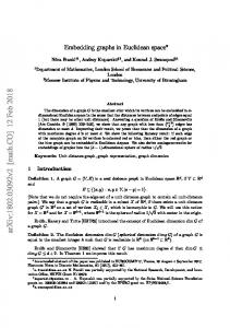
3. Scale-free Distribution of Nodes Although uniform distribution of nodes is assumed in most papers, it is not clear whether such distribution properly model the real word. People usually gather in groups and there are areas with high population density as well as areas which are sparsely populated. Thus, real network may not be represented by uniform distribution of nodes. In [9],[5] the distribution of population in cities is described. It is shown that urban population follows the power law N (w) ∼ w−γ , where N (w) is the number of cities with the population w. However the spatial distribution of population density is not considered. We analyzed the distribution of population density in a given area. We discovered that the density of population follows the power law. There is a small percent of the area with extremely high population and at the some time there is a large fraction of the area with relatively low population density. This idea may be observed in any scale: the world, country, province, city and finally even inside a building. The population density data are freely available on-line [1]. The area of continents is divided into small squares (size of about 20 km2 , for example there are 7833700 squares for Asia). The squares do not have equal size. The data contains for each square its area and population density. For our analysis we use data from the year 1995. 3.1 Population Density Distribution We analyze the probability P (d) that a given area has population density d. Two methods for measuring such distribution exists [5]: (I) direct measurement of probability density and (II) measurement of the cumulative distribution. Method (I) is performed by dividing the density scale into ranges and counting the percent of areas with densities within this range. In method (II) one selects a few density levels and for each level the area exceeding this population density is calculated. We selected the method (I). For densities smaller than 100 persons per km2 we use the ranges of 1, and above this density we use the range of 30 persons per km2 . Fig. 1 contains the probability P (d) measured for different continents. This probability follows the power-law with exponent γ about -2 for d > 100. For smaller d’s there is a cut off which courses that probability that area has population density d is smaller then predicted by the power-law.

100

100

Africa South America Asia

10

10

10-2

10-2

10-3

10-3

10-4

10-4

10-5

10-5

10-6

Europe North America Oceania

-1

Area

Area

-1

1

10

100

1000

10-6

1

10

Population Density

Figure 1. Probability P (d) measured for different continents. persons/km2 .

k 0 1 4 7 10 24

Continents North South Europe America America 1,000 1,000 1,000 0,896 0,944 0,969 0,726 0,773 0,811 0,609 0,517 0,677 0,517 0,491 0,515 0,318 0,289 0,300

100

1000

Population Density

σ = 0, 01 puni = 0 1,000 1,000 0,999 0,999 0,997 0,942

Population density is in

Model σ = 0, 01 σ = 0, 01 puni = 0, 3 puni = 0, 5 1,000 1,000 0,634 0,387 0,563 0,195 0,550 0,153 0,541 0,131 0,470 0,077

σ = 0, 01 puni = 1 1,000 0,335 0,111 0,068 0,047 0,023

Table 1. The density correlation for real data and some model parameters.

3.2 Correlation of Area Density and Neighborhood The second parameter we consider is the correlation between the density of area and average density of its neighborhood. Let Dr (x) be density in square x of size r. We also consider Dr,k (x) as an average density in squares with distance smaller than k to square x, where k is a parameter and r is a dimension of a square. Then we measure the correlation between Dr (x) and Dk (x) for a few values of k. As could be easily predicted this correlation is very high. This simply means that the neighborhood of the area having large density probably has a big population density, too. Table 1 presents the correlations obtained for Europe and North America and calculated for the model presented in the next section. Let us notice the analogies between this correlation parameter and clustering coefficient in scale free graphs.

4. Node’s Distribution Model To model the dynamics of population distribution as well as to obtain a good generator of such distributions we propose the following algorithm. We add nodes in the unit square [0, 1] × [0, 1]. Each nodes has coordinates (x, y), x ∈ (0, 1), y ∈ (0, 1). The model has two parameters punif orm , σ. We start with one node in the center of the square.

1: 2: 3: 4: 5: 6: 7: 8: 9:

V = {(0.5, 0.5)} for i ← 1, n − 1 do if u(0,1) < punif orm then add a new point to V with uniform coordinates probability distribution else randomly select an existing point with coordinates (x, y) ∈ V add new point to V with coordinates (x + N (0, σ), y + N (0, σ)) end if end for

Figure 2. The node’s coordinates generating algorithm. N (0, σ) denotes random variable with normal distribution with mean value 0 and variance σ. u(0,1) denotes uniformly distributed random variable in (0, 1).

The new node is added with probability punif orm uniformly in the square. Otherwise (with probability 1-punif orm ) an existing node is selected and a new one is added in its neighborhood defined by normal distribution with mean value 0 and variance σ. Figure 2 summarized the proposed algorithm.

Figure 3. Obtained data for n = 2000 nodes, n0 = 1. Left-top picture puniform =1, right-top picture puniform = 0.1,σ = 0.06, left-bottom picture puniform = 0.1,σ = 0.03, right-bottom picture puniform = 0.1,σ = 0.01.

Although it doesn’t look like at first sight, it is in fact a kind of preferential attachment

100

puni=0.01 puni=0.1 puni=0.3 puni=1

10-1

Area

10-2

10-3

10-4

10-5

10-6

1

10

100

1000

Number of points in cell

Figure 4. Probability P (d) measured for different model parameters. 4 × 106 nodes. We use 400000 squares in computations.

[3]. However, the probability of adding the node does not depends on the node degree. Instead it depends on the population(node) density in a given area. The area with more nodes, has bigger probability to be selected to get a new node. Fig. 4 presents P (d) for a few model parameters: punif orm = 1 simply denotes classical uniform distribution of nodes. As we change punif orm from 0 to 1 we move from scale free distribution towards uniform distribution of nodes. Similar properties are observed in classical scale free networks as we change from random to scale free graph. Fig. 3 presents examples of distributions of nodes for different model parameters.

5. The Complexity of TSP TSP belongs to N P-complete problems. Although N P-complete problems are believed to require exponential time to solve in the worst case, the typical-case behavior is usually difficult to characterize. For example, it was discovered [14] that N P-complete problems can exhibit phase transition phenomena, analogous to those in physical systems, with the hardest problems occurring at the phase boundary. In TSP, we consider a decision problem, namely if the path of length d exists. With randomly generated problems there is often a shape transition between two regions as the control parameter d is varied. In the constrained region, a very large number of solutions exist and it is relatively easily to find one. In the tightly constrained region, it is usually comparatively easy to show that no solution exists. Problems from the phase transition in between are typically hard since they cannot easily be proved soluble or insoluble. In our work we try to extent this approach. Instead of the decision problem we consider the optimization one and instead of path length d we use the model parameters punif orm and σ and try to identify the hardest problems for optimization. We used the Chained Lin-Kernigham algorithm with the implementation from the Concorde system [2]. This is a local-search heuristic. We compared the quality of obtained solutions with the lower bound computed by Concorde system. We checked instances with 5000 cities. For a set of model parameters we computed the average solution

0.35

σ=0.01 σ=0.025 σ=0.05 σ=0.075 σ=0.1

Percent Excess over Lower Bound

0.3

0.25

0.2

0.15

0.001

0.01

0.1

1

puni

Figure 5. Average difference between Lin-Kerningham solution and lower bound for TSP measured for different punif orm and σ parameters. 5000 cities. Difference between lower bound and heuristic solution in percents.

for 10 problem instances. Due to the fact that the Chained Lin-Kernigham algorithm is a stochastic method, for each problem we performed 10 independent runs. It turns out that local search procedure is very effective in solving the problem of such size. The difference is always below 1%. Although we were unable to find any phase transition we observed that the model parameters change the characteristic of the problem. The highest observed difference between the lower bound and heuristic solution was for punif orm = 0.1 and σ = 0.01 (Fig. 5) These are the most clustered problems. If we use bigger σ we obtain distributions which are similar to the uniform distribution od nodes. That’s why the chart for σ = 0.1 is flat.

6. Coloring of Unit Disk Graphs In this paper we also consider coloring of the unit disk graphs. To show the impact of our model on coloring of unit disk graphs we investigated several different coloring problems: • G(V, E) is a standard unit disk graph. Nodes coordinates are generated according to our model. Then the nodes with Euclidean distance smaller than r are connected. • G2 the square of unit disk graph i.e, the graph is build from G by adding edges connecting nodes at graph distance of 2. • G2 − G is the graph G2 without the edges of graph G Let us notice that graphs G2 are used to model wireless networks with primary and secondary conflicts. Graphs G2 − G are used to model networks with secondary conflicts only [11] [13]. Optimal coloring of these graphs determines the network resources needed for the conflict-free transmission (TDMA cycles length, CDMA codes or FDMA frequencies). We investigated four types of graph coloring algorithms: • Random greedy coloring with random ordering of vertices. • LF greedy coloring with ordering of vertices according to their degree. • DSATUR greedy coloring with dynamic vertices ordering according to saturation degree [7]. • branch and bound algorithm [7]. We use implementation described in [12].

200

12 G Rand G LF G DSATUR G branch and bound G2 Rand G2 LF G2 DSATUR G2 branch and bound

180

11

10

140

9

120

8

colors

colors

160

100

7

80

6

60

5

40

4

20

G2-G Rand G2-G LF G2-G dsatur G2-G branch and bound

3 0.1

0.2

0.3

0.4

0.5

0.6 puniform

0.7

0.8

0.9

1

0.1

0.2

0.3

0.4

0.5

0.6

0.7

0.8

0.9

1

puniform

Figure 6. The number of colors for G, G2 and G2 − G for different graph coloring algorithms and model parameters.

We checked networks with 250 nodes, r = 0.25, σ = 0.01. Parameter punif orm varies from 0.1 to 1 (i.e. from scale free distribution of nodes to standard uniform distribution). Fig. 6 presents the obtained results. Unfortunately not all graphs may be solved in reasonable time using branch and bound algorithm. Thus we stopped the algorithm after 109 backtracks and the best obtained result so far was used. As we may observe the hardest problems arise in the least realistic case of punif orm = 1. For punif orm = 1, G and G2 give almost 5 times smaller numbers of colors (network resources) for the uniform case than in more realistic case of punif orm = 0.1. On the other hand G2 − G graphs give larger number of colors for the uniform case, however the difference between the best heuristic (fast solution) and branch and bound algorithm became the largest (even 30 %). This kind of graphs seems to be the hardest for coloring.

7. Summary In the paper we analyzed the distribution of population density in Euclidean graphs. We showed that although these graphs are not scale-free, if we analyze the node’s degrees, the spatial distribution of nodes density follows the power law distribution. We presented a simple and efficient method of generating such distributions. Our model can be used in many areas of computer science dealing with Euclidean graphs. We analyzed the impact of such model on two different problems TSP and coloring of conflict graphs in wireless networks. We showed that these graphs behaves differently than standard unit disk graphs with uniform distribution. The TSP problem is the most difficult if many clusters appear. On the other hand coloring of conflicts graphs is harder with the uniform distributed nodes. We also observed huge difference between the number of colors (network resources) needed in scale free and uniform distribution of nodes. Future work is to find similar properties for other problems, for example minimal connected dominating set used in wireless networks routing. The known bounds for chromatic number of unit disk graphs may also be extended. Let us notice that in this work we consider only static graphs. In wireless networks nodes may move. Good mobility models and distributed algorithms based on our model of distribution of nodes are also possible.

Bibliography [1] Gridded population of the world (gpw) data set. Columbia University; International Food Policy Research Institute (IFPRI); and World Resources Institute (WRI). Available at http://sedac.ciesin.columbia.edu/plue/gpw, 1995. [2] Concorde tsp solver. Available at http://www.tsp.gatech.edu/concorde.htmlAvailable, 2000. [3] Reka Albert and Albert-Laszlo Barabasi. Statistical mechanics of complex networks. Review of Modern Physics, pages 47–97, January 2002. [4] Albert-Laszlo Barabasi and Zoltan N. Oltvai. Network biology: Understanding the cell’s functional organization. Nature, pages 101–113, February 2004. [5] Aharon Blank and Sorin Solomon. Power laws and cities population. http://arxiv.org/html/cond-mat/0003240, 2000. [6] J.M Braun M.L., Buhmann. The noisy euclidean traveling salesman problem and learning. Advances in Neural Information Processing Systems, 2002. [7] D. Brelaz. New methods to color vertices of a graph. Communications of the ACM, 22:251–256, 1979. [8] Brent N. Clark, Charles J. Colbourn, and David S. Johnson. Unit disk graphs. Discrete Math., 86(1-3):165–177, 1990. [9] G.Zipf. Human behavior and the principles of last effort. 1949. [10] D. Johnson and M. A. McGeoch. The Traveling Salesman Problem and its Variations, chapter Experimental analysis of heuristics for the STSP. Kluwer Academic Publishers, 2002. [11] E.L. Lloyd. Broadcast scheduling for tdma in wireless multihop networks. Handbook of Wireless Networks and Mobile Computing, pages 347–370, 2002. [12] A. Mehrotra and M. A. Trick. A column generation approach to graph coloring. Technical report, Carnegie Mellon Univercity, 1995. [13] A. A.Bertossi R. Battoti and M. A. Bonuccelli. Assigning codes in wireless networks: Bounds and scaling properties. Wireless Networks, pages Vol. 5, 195–209, 1999. [14] S.Krirkpatick-B. Selman R. Monasson, R. Zecchina and L. Troyansky. Determining computational complexity from characteristic ’phase transition’. Nature, 400:133– 137, 1999. [15] Albert-Laszlo Barabasi Reka Albert, Hawoong Jeong. Diameter of the world-wide web. Nature, page 130, September 1999. [16] Jano I. van Hemert and Neil B. Urquhart. Phase transition properties of clustered traveling salesman problem instances generated with evolutionary computation. In Parallel Problem Solvers from Nature VIII, pages 150–159, 2004. [17] Xiao Fan Wang and Guanrong Chen. Complex networks: Small-word, scale-free and beyond. IEEE Circuits and Systems Magazine, pages 6–20, First quarter 2003.