SCALING FOR A ONE-DIMENSIONAL DIRECTED POLYMER WITH

arXiv:0911.2446v2 [math.PR] 13 Jan 2010

SCALING FOR A ONE-DIMENSIONAL DIRECTED POLYMER WITH BOUNDARY CONDITIONS ¨ AINEN ¨ TIMO SEPPAL Abstract. We study a 1 + 1-dimensional directed polymer in a random environment on the integer lattice with log-gamma distributed weights and both endpoints of the path fixed. Among directed polymers this model is special in the same way as the last-passage percolation model with exponential or geometric weights is special among growth models, namely, both permit explicit calculations. With appropriate boundary conditions the polymer with log-gamma weights satisfies an analogue of Burke’s theorem for queues. Building on this we prove that the fluctuation exponents for the free energy and the polymer path have their conjectured values. For the polymer without boundary conditions and with either fixed or free endpoint we get the expected upper bounds on the exponents.

1. Introduction The directed polymer in a random environment represents a polymer (a long chain of molecules) by a random walk path that interacts with a random environment. Let x = (xk )k≥0 denote a nearest-neighbor path in Zd started at the origin: xk ∈ Zd , x0 = 0, and |xk − xk−1 | = 1. The environment ω = (ω(s, u) : s ∈ N, u ∈ Zd ) puts a real-valued weight ω(s, u) at space-time point (u, s) ∈ Zd × N. For a path segment x0,n = P(x0 , . . . , xn ), Hn (x0,n ) is the total weight collected by the walk up to time n: Hn (x0,n ) = ns=1 ω(s, xs ). The quenched polymer distribution on paths, in environment ω and at inverse temperature β > 0, is the probability measure defined by 1 (1.1) Qωn (dx ) = ω exp{βHn (x0,n )} Zn P with normalization factor (partition function) Znω = x0,n eβHn (x0,n ) . The environment ω is taken as random with probability distribution P, typically such that the weights {ω(s, u)} are i.i.d. random variables. At β = 0 the model is standard simple random walk. The general objective is to understand how the model behaves as β > 0 and the dimension d varies. A key question is whether the diffusive behavior of the walk is affected. “Diffusive behavior” refers to the fluctuation behavior of standard random walk, characterized by n−1 E(x2n ) → c and convergence of diffusively rescaled walks n−1/2 x⌊nt⌋ to Brownian motion. Date: January 13, 2010. 2000 Mathematics Subject Classification. 60K35, 60K37, 82B41, 82D60. Key words and phrases. scaling exponent, directed polymer, random environment, superdiffusivity, Burke’s theorem, partition function. T. Sepp¨ al¨ ainen was partially supported by National Science Foundation grant DMS-0701091 and by the Wisconsin Alumni Research Foundation. 1

¨ AINEN ¨ T. SEPPAL

2

The directed polymer model was introduced in the statistical physics literature by Huse and Henley in 1985 [14]. The first rigorous mathematical work was by Imbrie and Spencer [15] in 1988. They proved with an elaborate expansion that in dimensions d ≥ 3 and with small enough β, the walk is diffusive in the sense that, for a.e. environment ω, ω n−1 E Q (|xn |2 ) → c. Bolthausen [7] strengthened the result to a central limit theorem for the endpoint of the walk, still d ≥ 3, small β and for a.e. ω, through the observation that Wn = Zn /E(Zn ) is a martingale. Since then martingale techniques have been a standard fixture in much of the work on directed polymers. The limit W∞ = lim Wn is either almost surely 0 or almost surely > 0. The case W∞ = 0 has been termed strong disorder and W∞ > 0 weak disorder. There is a critical value βc such that weak disorder holds for β < βc and strong for β > βc . It is known that βc = 0 for d ∈ {1, 2} and 0 < βc ≤ ∞ for d ≥ 3. In d ≥ 3 and weak disorder the walk converges to a Brownian motion, and the limiting diffusion matrix is the same as for standard random walk [12]. There is a further refinement of strong disorder into strong and very strong disorder. Sharp recent results appear in [20]. One way to phrase questions about the polymer model is to ask about two scaling exponents, ζ and χ, defined somewhat informally as follows: (1.2)

fluctuations of the path x0,n are of order nζ

and (1.3)

fluctuations of log Zn are of order nχ .

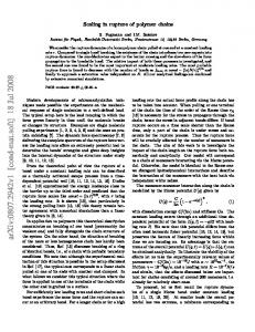
Let us restrict ourselves to the case d = 1 for the remainder of the paper. By the results mentioned above the model is in strong disorder for all β > 0. It is expected that the 1-dimensional exponents are χ = 1/3 and ζ = 2/3 [19]. Precise values have not been obtained in the past, but during the last decade nontrivial rigorous bounds have appeared in the literature for some models with Gaussian ingredients. For a Gaussian random walk in a Gaussian potential Petermann [26] proved the lower bound ζ ≥ 3/5 and Mejane [23] provided the upper bound ζ ≤ 3/4. Petermann’s proof was adapted to a certain continuous setting in [6]. For an undirected Brownian motion in a Poissonian potential W¨ uthrich obtained 3/5 ≤ ζ ≤ 3/4 and χ ≥ 1/8 [30, 31]. For a directed Brownian motion in a Poissonian potential Comets and Yoshida derived ζ ≤ 3/4 and χ ≥ 1/8 [11]. Piza [27] showed generally that the fluctuations of log Zn diverge at least logarithmically, and bounds on exponents under curvature assumptions on the limiting free energy. Related results for first passage percolation appeared in [21, 24]. For the rest of the discussion we turn the picture 45 degrees clockwise so that the model lives in the nonnegative quadrant Z2+ of the plane, instead of the space-time wedge {(u, s) ∈ Z×N : |u| ≤ s}. The weights are i.i.d. variables {ω(i, j) : i, j ≥ 0}. The polymer x becomes a nearest-neighbor up-right path (see Figure 1). We also fix both endpoints of the path. So, given the endpoint (m, n), the partition function is (1.4)

ω Zm,n =

X

x0,m+n

n m+n o X exp β ω(xk ) k=1

SCALING FOR A POLYMER

y

6

•

5

6

•

4

6

• -• -• -•

3

6

•

2

6

•

1 0

3

6

• -• -• 0

1

2

3

4

5

- x

Figure 1. An up-right path from (0, 0) to (5, 5) in Z2+ . where the sum is over paths x0,m+n that satisfy x0 = (0, 0), xm+n = (m, n) and xk − xk−1 = (1, 0) or (0, 1). The polymer measure of such a path is (1.5)

Qωm,n (x0,m+n ) =

1 ω Zm,n

o n m+n X ω(xk ) . exp β k=1

If we take the “zero temperature limit” β ր ∞ in (1.5) then the measure Qωm,n concenP trates on the path x0,m+n that maximizes the sum m+n k=1 ω(xk ). Thus the polymer model has become a last-passage percolation model, also called the corner growth model. The quantity that corresponds to log Zm,n is the passage time (1.6)

Gm,n = max

x0,m+n

m+n X

ω(xk ).

k=1

For certain last-passage growth models, notably for (1.6) with exponential or geometric weights ω(i, j), not only have the predicted exponents been confirmed but also limiting Tracy-Widom fluctuations for Gm,n have been proved [3, 4, 10, 13, 16, 17]. The recent article [5] verifies a complete picture proposed in [28] that characterizes the scaling limits of Gm,n with exponential weights as a function of the parameters of the boundary weights and the ratio m/n. In the present paper we study the polymer model (1.4)–(1.5) with fixed endpoints, with fixed β = 1, and for a particular choice of weight distribution. Namely, the weights {ω(i, j)} are independent random variables with log-gamma distributions. Precise definitions follow in the next section. This particular polymer model turns out to be amenable to explicit computation, similarly to the case of exponential or geometric weights among the corner growth models (1.6). We introduce a polymer model with boundary conditions that possesses a two-dimensional stationarity property. By boundary conditions we mean that the weights on the boundaries of Z2+ are distributionally different from the weights in the interior, or bulk. For the model with boundary conditions we prove that the fluctuation exponents take exactly their conjectured values χ = 1/3 and ζ = 2/3 when the endpoint (m, n) is taken to infinity along a

4

¨ AINEN ¨ T. SEPPAL

characterictic direction. This characteristic direction is a function of the parameters of the weight distributions. In other directions log Zm,n satisfies a central limit theorem in the model with boundary conditions. As a corollary we get the correct upper bounds for the exponents in the model without boundary and with either fixed or free endpoint, but still with i.i.d. log-gamma weights {ω(i, j)}. In addition to the β ր ∞ limit, there is another formal connection between the polymer model and the corner growth model. Namely, the definitions of Zm,n and Gm,n imply the equations (1.7)

Zm,n = eβω(m,n) (Zm−1,n + Zm,n−1 )

and (1.8)

Gm,n = ω(m, n) + max(Gm−1,n , Gm,n−1 ).

These equations can be paraphrased by saying that Gm,n obeys max-plus algebra, while Zm,n obeys the familiar algebra of addition and multiplication. This observation informs the approach of the paper. It is not that we can convert results for G into results for Z. Rather, after the proofs have been found, one can detect a kinship with the arguments of [4], but transformed from (max, +) to (+ , · ). The ideas in [4] were originally adapted from the seminal paper [10]. The purpose was to give an alternative proof of the scaling exponents of the corner growth model, without the asymptotic analysis of Fredholm determinants utilized in [16]. Frequently used notation. N = {1, 2, 3, . . . } and Z+ = {0, 1, 2, . . . }. Rectangles on the planar integer lattice are denoted by Λm,n = {0, . . . , m} × {0, . . . , n} and more generally Λ(k,ℓ),(m,n) = {k, . . . , m} × {ℓ, . . . , n}. P is the probability distribution on the random environments or weights ω, and under P the expectation of a random variable X is E(X) and variance Var(X). Overline means centering: X = X −EX. Qω is the quenched polymer measure in a rectangle. The annealed measure is P (·) = EQω (·) with expectation E(·). P is used for a generic probability measure that is not part of the polymer model. Paths can be written xk,ℓ = (xk , xk+1 , . . . , xℓ ) but also x when k, ℓ are understood. Acknowledgement. The author thanks M´arton Bal´azs for pointing out that the gamma distribution solves the equations of Lemma 3.2 and Persi Diaconis for literature suggestions. 2. The model and results We begin with the definition of the polymer model with boundaries and then state the results. As stated in the introduction, relative to the standard description of the polymer model we turn the picture 45 degrees clockwise so that the polymer lives in the nonnegative quadrant Z2+ of the planar lattice. The inverse temperature parameter β = 1 throughout. We replace the exponentiated weights with multiplicative weights Yi,j = eω(i,j) , (i, j) ∈ Z2+ . Then the partition function for paths whose endpoint is constrained to lie at (m, n) is given by (2.1)

Zm,n =

X

m+n Y

x ∈Πm,n k=1

Yxk

SCALING FOR A POLYMER

5

where Πm,n denotes the collection of up-right paths x = (xk )0≤k≤m+n inside the rectangle Λm,n = {0, . . . , m} × {0, . . . , n} that go from (0, 0) to (m, n): x0 = (0, 0), xm+n = (m, n) and xk − xk−1 = (1, 0) or (0, 1). We adopt the convention that Zm,n does not include the weight at the origin, and if a value is needed then set Z0,0 = Y0,0 = 1. The symbol ω will denote the entire random environment: ω = (Yi,j : (i, j) ∈ Z2+ ). When necessary the ω , with a similar convention for other dependence of Zm,n on ω will be expressed by Zm,n ω-dependent quantities. We assign distinct weight distributions on the boundaries (N × {0}) ∪ ({0} × N) and in the bulk N2 . To highlight this the symbols U and V will denote weights on the horizontal and vertical boundaries: (2.2)

Ui,0 = Yi,0

and V0,j = Y0,j

for i, j ∈ N.

However, in formulas such as (2.1) it is obviously convenient to use a single symbol Yi,j for all the weights. Our results rest on the assumption that the weights are reciprocals of gamma variables. R∞ Let us recall some basics. The gamma function is Γ(s) = 0 xs−1 e−x dx. We shall need it only for positive real s. The Gamma(θ, r) distribution has density Γ(θ)−1 r θ xθ−1 e−rx on R+ , mean θ/r and variance θ/r 2 . The logarithm log Γ(s) is convex and infinitely differentiable on (0, ∞). The derivatives are the polygamma functions Ψn (s) = (dn+1 /dsn+1 ) log Γ(s), n ∈ Z+ [1, Section 6.4]. For n ≥ 1, Ψn is nonzero and has sign (−1)n−1 throughout (0, ∞) [29, Thm. 7.71]. Throughout the paper we make use of the digamma and trigamma functions Ψ0 and Ψ1 , on account of the connections (2.3)

Ψ0 (θ) = E(log A)

and Ψ1 (θ) = Var(log A) for

A ∼ Gamma(θ, 1).

Here is the assumption on the distributions. Let 0 < θ < µ < ∞. (2.4)

Weights {Ui,0 , V0,j , Yi,j : i, j ∈ N} are independent with distributions

−1 −1 −1 Ui,0 ∼ Gamma(θ, 1), V0,j ∼ Gamma(µ − θ, 1), and Yi,j ∼ Gamma(µ, 1).

We fixed the scale parameter r = 1 in the gamma distributions above for the sake of convenience. We could equally well fix it to any value and our results would not change, as long as all three gamma distributions above have the same scale parameter. A key technical result will be that under (2.4) each ratio Um,n = Zm,n /Zm−1,n and Vm,n = Zm,n /Zm,n−1 has the same marginal distribution as U and V in (2.4). This is a Burke’s Theorem of sorts, and appears as Theorem 3.3 below. From this we can compute the mean exactly: for m, n ≥ 0,   (2.5) E log Zm,n = mE(log U ) + nE(log V ) = −mΨ0 (θ) − nΨ0 (µ − θ). Together with the choice of the parameters θ, µ goes a choice of “characteristic direction” (Ψ1 (µ − θ), Ψ1 (θ)) for the polymer. Let N denote the scaling parameter we take to ∞. We assume that the coordinates (m, n) of the endpoint of the polymer satisfy (2.6)

| m − N Ψ1 (µ − θ) | ≤ γN 2/3

and

| n − N Ψ1 (θ) | ≤ γN 2/3

for some fixed constant γ. Now we can state the variance bounds for the free energy.

¨ AINEN ¨ T. SEPPAL

6

Theorem 2.1. Assume (2.4) and let (m, n) be as in (2.6). Then there exist constants 0 < C1 , C2 < ∞ such that, for N ≥ 1, C1 N 2/3 ≤ Var(log Zm,n ) ≤ C2 N 2/3 .

The constants C1 , C2 in the theorem depend on 0 < θ < µ and on γ of (2.6), and they can be taken the same for (θ, µ, γ) that vary in a compact set. This holds for all the constants in the theorems of this section: they depend on the parameters of the assumptions, but for parameter values in a compact set the constants themselves can be fixed. The upper bound on the variance is good enough for Borel-Cantelli to give the strong law of large numbers: with (m, n) as in (2.6), (2.7)

lim N −1 log Zm,n = −Ψ0 (θ)Ψ1 (µ − θ) − Ψ0 (µ − θ)Ψ1 (θ) P-a.s.

N →∞

As a further corollary we deduce that if the direction of the polymer deviates from the characteristic one by a larger power of N than allowed by (2.6), then log Z satisfies a central limit theorem. For the sake of concreteness we treat the case where the horizontal direction is too large. Corollary 2.2. Assume (2.4). Suppose m, n → ∞. Define parameter N by n = Ψ1 (θ)N , and assume that
N −α m − Ψ1 (µ − θ)N → c1 > 0 as N → ∞ for some α > 2/3. Then as N → ∞, n
o N −α/2 log Zm,n − E log Zm,n

converges in distribution to a centered normal distribution with variance c1 Ψ1 (θ). The quenched polymer measure Qωm,n is defined on paths x ∈ Πm,n by (2.8)

Qωm,n (x )

=

1 Zm,n

m+n Y

Yxk

k=1

remembering convention (2.2). Integrating out the random environment ω gives the annealed measure Z Pm,n (x ) = Qωm,n (x ) P(dω).

When the rectangle Λm,n is understood, we drop the subscripts and write P = EQω . Notation will be further simplified by writing Q for Qω . We describe the fluctuations of the path x under P . The next result shows that N 2/3 is the exact order of magnitude of the fluctuations of the path. Let v0 (j) and v1 (j) denote the left- and rightmost points of the path on the horizontal line with ordinate j: (2.9)

v0 (j) = min{i ∈ {0, . . . , m} : ∃k : xk = (i, j)}

and (2.10)

v1 (j) = max{i ∈ {0, . . . , m} : ∃k : xk = (i, j)}.

SCALING FOR A POLYMER

7

Theorem 2.3. Assume (2.4) and let (m, n) be as in (2.6). Let 0 ≤ τ < 1. Then there exist constants C1 , C2 < ∞ such that for N ≥ 1 and b ≥ C1 ,  (2.11) P v0 (⌊τ n⌋) < τ m − bN 2/3 or v1 (⌊τ n⌋) > τ m + bN 2/3 ≤ C2 b−3 .

Same bound holds for the vertical counterparts of v0 and v1 . Let 0 < τ < 1. Then given ε > 0, there exists δ > 0 such that (2.12)

lim P { ∃k such that | xk − (τ m, τ n)| ≤ δN 2/3 } ≤ ε.

N →∞

We do not have a quenched result this sharp. From Lemma 4.3 and the proof of Theorem 2.3 in Section 6 one can extract estimates on the P-tails of the quenched probabilities of the events in (2.11) and (2.12). We turn to results for the model without boundaries, by restricting ourselves to the positive quadrant N2 . Define the partition function of a general rectangle {k, . . . , m} × {ℓ, . . . , n} by (2.13)

Z(k,ℓ),(m,n) =

X

x ∈Π(k,ℓ),(m,n)

m−k+n−ℓ Y

Yxi

i=1

m−k+n−ℓ where Π(k,ℓ),(m,n) is the collection of up-right paths x = (xi )i=0 from x0 = (k, ℓ) to xm−k+n−ℓ = (m, n). Admissible steps are always xi+1 − xi = e1 = (1, 0) or xi+1 − xi = e2 = (0, 1). We have chosen not to include the weight of the southwest corner (k, ℓ). The earlier definition (2.1) is the special case Zm,n = Z(0,0),(m,n) . Also we stipulate that when the rectangle reduces to a point, Z(k,ℓ),(k,ℓ) = 1. In particular, Z(1,1),(m,n) gives us partition functions that only involve the bulk weights {Yi,j : i, j ∈ N}. The assumption on their distribution is as before, with a fixed parameter 0 < µ < ∞:

(2.14)

−1 ∼ Gamma(µ, 1). {Yi,j : i, j ∈ N} are i.i.d. with common distribution Yi,j

We define the limiting free energy. The identity (see e.g. [2, (2.11)] or [1, Section 6.4]) Ψ1 (x) =

∞ X k=0

1 (x + k)2

shows that Ψ1 (0+) = ∞. Thus, given 0 < s, t < ∞, there is a unique θ = θs,t ∈ (0, µ) such that s Ψ1 (µ − θ) = . (2.15) Ψ1 (θ) t Define (2.16)


fs,t(µ) = − sΨ0 (θs,t ) + tΨ0 (µ − θs,t) .

It can be verified that for a fixed 0 < µ < ∞, fs,t (µ) is a continuous function of (s, t) ∈ R2+ with boundary values f0,t (µ) = ft,0 (µ) = −tΨ0 (µ).

¨ AINEN ¨ T. SEPPAL

8

Here is the result for the free energy of the polymer without boundary but still with fixed endpoint. Assume the endpoint (m, n) satisfies (2.17)

|m − N s| ≤ γN 2/3

and

|n − N t| ≤ γN 2/3

for a constant γ. The constants in this theorem and the next depend on (s, t, µ, γ). Theorem 2.4. Assume (2.14) and let 0 < s, t < ∞. We have the law of large numbers (2.18)

lim N −1 log Z(1,1),(⌊N s⌋,⌊N t⌋) = fs,t(µ)

P-a.s.

N →∞

Assume (m, n) satisfies (2.17). There exist finite constants N0 and C0 such that, for b ≥ 1 and N ≥ N0 ,   (2.19) P | log Z(1,1),(m,n) − N fs,t(µ)| ≥ bN 1/3 ≤ C0 b−3/2 . In particular, we get the moment bound   log Z(1,1),(⌊N s⌋,⌊N t⌋) − N fs,t (µ) p ≤ C(s, t, µ, γ, p) < ∞ (2.20) E N 1/3

for N ≥ N0 (s, t, µ, γ) and 1 ≤ p < 3/2. The theorem is proved by relating Z(1,1),(m,n) to a polymer with a boundary. Equation (2.15) picks the correct boundary parameter θ. Presently we do not have a matching lower bound for (2.19). In a general rectangle the quenched polymer distribution of a path x ∈ Π(k,ℓ),(m,n) is (2.21)

Q(k,ℓ),(m,n) (x ) =

1 Z(k,ℓ),(m,n)

m−k+n−ℓ Y

Yxi .

i=1

As before the annealed distribution is P(k,ℓ),(m,n) (·) = EQ(k,ℓ),(m,n) (·). The upper fluctuation bounds for the path in the model with boundaries can be extended to the model without boundaries. Theorem 2.5. Assume (2.14), fix 0 < s, t < ∞, and assume (2.17). Let 0 ≤ τ < 1. Then there exist finite constants C, C0 and N0 such that for N ≥ N0 and b ≥ C0 ,  P(1,1),(⌊N s⌋,⌊N t⌋) v0 (⌊τ N t⌋) < τ N s − bN 2/3 (2.22) or v1 (⌊τ N t⌋) > τ N s + bN 2/3 ≤ Cb−3 .

Same bound holds for the vertical counterparts of v0 and v1 .

Next we drop the restriction on the endpoint, and extend the upper bounds to the polymer with unrestricted endpoint and no boundaries. Given the value of the parameter N ∈ N, the set of admissible paths is ∪1≤k≤N −1 Π(1,1),(k,N −k) , namely the set of all up-right paths x = (xk )0≤k≤N −2 that start at x0 = (1, 1) and whose endpoint xN −2 lies on the line x + y = N . The quenched polymer probability of such a path is Qtot N (x ) =

N −2 1 Y Yxk tot ZN k=1

SCALING FOR A POLYMER

9

with the “total” partition function tot ZN =

N −1 X

Z(1,1),(k,N −k) .

k=1

PNtot (·)

EQtot N (·).

The annealed measure is = We collect all the results in one theorem, proved in Section 8. In particular, (2.25) below shows that the fluctuations of the endpoint of the path are of order at most N 2/3 . Statement (8.20) in the proof gives bounds on the quenched probability of a deviation. Theorem 2.6. Fix 0 < µ < ∞ and assume weight distribution (2.14). We have the law of large numbers (2.23)

tot lim N −1 log ZN = f1/2,1/2 (µ) = −Ψ0 (µ/2)

P-a.s.

N →∞

Let C(µ) be a constant that depends on µ alone. For b ≥ 1 there exists N0 (µ, b) < ∞ such that   tot (2.24) sup P | log ZN − N f1/2,1/2 (µ)| ≥ bN 1/3 ≤ C(µ)b−3/2 N ≥N0 (µ,b)

and

(2.25)

sup N ≥N0 (µ,b)

 PNtot xN −2 − ( N2 , N2 ) ≥ bN 2/3 ≤ C(µ)b−3 .

The last case to address is the polymer with boundaries but free endpoint. This case is perhaps of less interest than the others for the free energy scales diffusively, but we record it for the sake of completeness. Fix 0 < θ < µ and let assumption (2.4) on the weight distributions be in force. The fixed-endpoint partition function Zm,n = Z(0,0),(m,n) is the one defined in (2.1). Define the partition function of all paths from (0, 0) to the line x + y = N by N X tot ZN (θ, µ) = Zℓ,N −ℓ . ℓ=0

Define a limiting free energy


g(θ, µ) = max −sΨ0 (θ) − (1 − s)Ψ0 (µ − θ) = 0≤s≤1

Set also

(

−Ψ0 (θ) θ ≤ µ/2 −Ψ0 (µ − θ) θ ≥ µ/2.

( Ψ1 (θ) θ ≤ µ/2 σ 2 (θ, µ) = Ψ1 (µ − θ) θ ≥ µ/2,

and define random variables ζ(θ, µ) as follows: for θ 6= µ/2, ζ(θ, µ) has centered normal distribution with variance σ 2 (θ, µ), while p
′ (2.26) ζ(µ/2, µ) = 2Ψ1 (µ/2) M1/2 ∨ M1/2

where Mt = sup0≤s≤t B(s) is the running maximum of a standard Brownian motion and Mt′ is an independent copy of it.

¨ AINEN ¨ T. SEPPAL

10

Theorem 2.7. Let 0 < θ < µ and assume (2.4). We have the law of large numbers tot lim N −1 log ZN (θ, µ) = g(θ, µ)

(2.27)

P-a.s.

N →∞

and the distributional limit (2.28)


d tot N −1/2 log ZN (θ, µ) − N g(µ/2, µ) −→ ζ(θ, µ).

When θ 6= µ/2 the axis with the larger −Ψ0 value completely dominates, while if θ = µ/2 all directions have the same limiting free energy. This accounts for the results in the theorem. Organization of the paper. Before we begin the proofs of the main theorems, Section 3 collects basic properties of the model, including the Burke-type property. The upper and lower bounds of Theorem 2.1 are proved in Sections 4 and 5. Corollary 2.2 is proved at the end of Section 4. The bounds for the fixed-endpoint path with boundaries are proved in Section 6, and the results for the fixed-endpoint polymer model without boundaries in Section 7. The results for the polymer with free endpoint are proved in Section 8. 3. Basic properties of the polymer model with boundaries This section sets the stage for the proofs with some preliminaries. The main results of this section are the Burke property in Theorem 3.3 and identities that tie together the variance of the free energy and the exit points from the axes in Theorem 3.7. Occasionally we will use notation for the partition function that includes the weight at the starting point, which we write as (3.1)



Z(i,j),(k,ℓ) =

X

x ∈Π(i,j),(k,ℓ)

k−i+ℓ−j Y

Yxr = Yi,j Z(i,j),(k,ℓ) .

r=0

Let the initial weights {Ui,0 , V0,j , Yi,j : i, j ∈ N} be given. Starting from the lower left corner of N2 , define inductively for (i, j) ∈ N2   Vi−1,j  Ui,j−1  , Vi,j = Yi,j 1 + Ui,j = Yi,j 1 + Vi−1,j Ui,j−1 (3.2)  1 1 −1 + and Xi−1,j−1 = . Ui,j−1 Vi−1,j

The partition function satisfies (3.3)

Zm,n = Ym,n Zm−1,n + Zm,n−1

and one checks inductively that (3.4)

Um,n =

Zm,n Zm−1,n

and




for (m, n) ∈ N2

Vm,n =

Zm,n Zm,n−1

 for (m, n) ∈ Z2+ r {(0, 0)}. Equations (3.3) and (3.4) are also valid for Zm,n because the weight at the origin cancels from the equations.

SCALING FOR A POLYMER

11

It is also natural to associate the U - and V -variables to undirected edges of the lattice Z2+ . If f = {x − e1 , x} is a horizontal edge then Tf = Ux , while if f = {x − e2 , x} then Tf = Vx . The following monotonicity property can be proved inductively: Lemma 3.1. Consider two sets of positive initial values {Ui,0 , V0,j , Yi,j : i, j ∈ N} and ei,0 , Ve0,j , Yei,j : i, j ∈ N} that satisfy Ui,0 ≥ U ei,0 , V0,j ≤ Ve0,j , and Yi,j = Yei,j . From these {U ei,j , Vei,j : (i, j) ∈ N2 } by equation define inductively the values {Ui,j , Vi,j : (i, j) ∈ N2 } and {U ei,j and Vi,j ≤ Vei,j for all (i, j) ∈ N2 . (3.2). Then Ui,j ≥ U

3.1. Propagation of boundary conditions. The next lemma gives a reversibility property that we can regard as an analogue of reversibility properties of M/M/1 queues and their last-passage versions. (A basic reference for queues is [18]. Related work appears in [4, 9, 10, 25].) Lemma 3.2. Let U , V and Y be independent positive random variables. Define (3.5)

U ′ = Y (1 + U V −1 ),

V ′ = Y (1 + V U −1 )

and

Y ′ = (U −1 + V −1 )−1 .

Then the triple (U ′ , V ′ , Y ′ ) has the same distribution as (U, V, Y ) iff there exist positive parameters 0 < θ < µ and r such that (3.6)

U −1 ∼ Gamma(θ, r), V −1 ∼ Gamma(µ − θ, r), and Y −1 ∼ Gamma(µ, r).

Proof. Assuming (3.6), define independent gamma variables A = U −1 , B = V −1 and Z = Y −1 . Then set ZA ZB A′ = , B′ = , and Z ′ = A + B. A+B A+B d

We need to show that (A′ , B ′ , Z ′ ) = (A, B, Z). Direct calculation with Laplace transforms is convenient. Alternatively, one can reason with basic properties of gamma distributions as follows. The pair (A/(A+B), B/(A+B)) has distributions Beta(θ, µ−θ) and Beta(µ−θ, θ), and is independent of the Gamma(µ, r)-distributed sum A + B = Z ′ . Hence A′ and B ′ are a pair of independent variables with distributions Gamma(θ, r) and Gamma(µ − θ, r), and by construction also independent of Z ′ . d Assuming (A′ , B ′ , Z ′ ) = (A, B, Z), A′ /B ′ = A/B is independent of Z ′ = A + B. By Theorem 1 of [22] A and B are independent gamma variables with the same scale parameter d

r. Then Z = Z ′ = A + B determines the distribution of Z.



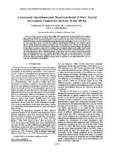
From this lemma we get a Burke-type theorem. Let z = (zk )k∈Z be a nearest-neighbor down-right path in Z2+ , that is, zk ∈ Z2+ and zk − zk−1 = e1 or −e2 . Denote the undirected edges of the path by fk = {zk−1 , zk }, and let ( Uz k if fk is a horizontal edge Tfk = Vzk−1 if fk is a vertical edge.

¨ AINEN ¨ T. SEPPAL

12

••• ••• ••• ••• ••• ••• ••• •••

an edge fk = {zk−1 , zk } of the down-right path

•

an interior point

Figure 2. Illustration of a down-right path (zk ) and its set I of interior points. Let the (lower left) interior of the path be the vertex set I = {(i, j) ∈ Z2+ : ∃m ∈ N : (i + m, j + m) ∈ {zk }} (see Figure 2). I is finite if the path z coincides with the axes for all but finitely many edges. Recall the definition of Xi,j from (3.2). Theorem 3.3. Assume (2.4). For any down-right path (zk )k∈Z in Z2+ , the variables {Tfk , Xz : k ∈ Z, z ∈ I} are mutually independent with marginal distributions (3.7)

U −1 ∼ Gamma(θ, 1), V −1 ∼ Gamma(µ − θ, 1), and X −1 ∼ Gamma(µ, 1).

Proof. This is proved first by induction for down-right paths with finite interior I. If z coincides with the x- and y-axes then I is empty, and the statement follows from assumption (2.4). The inductive step consists of adding a “growth corner” to I and an application of Lemma 3.2. Namely, suppose z goes through the three points (i − 1, j), (i − 1, j − 1) and (i, j − 1). Flip the corner over to create a new path z′ that goes through (i − 1, j), (i, j) and (i, j − 1). The new interior is I ′ = I ∪ {(i − 1, j − 1)}. Apply Lemma 3.2 with U = Ui,j−1 , V = Vi−1,j , Y = Yi,j , U ′ = Ui,j , V ′ = Vi,j , and Y ′ = Xi−1,j−1

to see that the conclusion continues to hold for z′ and I ′ . To prove the theorem for an arbitrary down-right path it suffices to consider a finite portion of z and I inside some large square B = {0, . . . , M }2 . Apply the first part of the proof to the modified path that coincides with z inside B but otherwise follows the coordinate axes and connects up with z on the north and east boundaries of B.  To understand the sense in which Theorem 3.3 is a “Burke property”, note its similarity with Lemma 4.2 in [4] whose connection with M/M/1 queues in series is immediate through the last-passage representation. 3.2. Reversal. In a fixed rectangle Λ = {0, . . . , m}×{0, . . . , n} define the reversed partition function Zm,n ∗ for (i, j) ∈ Λ. (3.8) Zi,j = Zm−i,n−j Note that for the partition function of the entire rectangle, ∗ Zm,n = Zm,n .

SCALING FOR A POLYMER

13

Recalling (3.2) make these further definitions: ∗ Ui,j = Um−i+1,n−j

(3.9)

∗ Vi,j ∗ Yi,j

= Vm−i,n−j+1 = Xm−i,n−j

for (i, j) ∈ {1, . . . , m} × {0, . . . , n},

for (i, j) ∈ {0, . . . , m} × {1, . . . , n},

for (i, j) ∈ {1, . . . , m} × {1, . . . , n}.

∗∗ = Z The mapping ∗ is an involution, that is, inside the rectangle Λ, Zi,j i,j and similarly for U , V and Y .

Proposition 3.4. Assume distributions (2.4). Then inside the rectangle Λ the system ∗ , U ∗ , V ∗ , Y ∗ } replicates the properties of the original system {Z , U , V , Y }. Namely, {Zi,j i,j i,j i,j i,j i,j i,j i,j we have these facts: ∗ , V ∗ , Y ∗ : 1 ≤ i ≤ m, 1 ≤ j ≤ n} are independent with distributions (a) {Ui,0 0,j i,j (3.10)

∗ −1 ∗ −1 (Ui,0 ) ∼ Gamma(θ, 1), (V0,j ) ∼ Gamma(µ − θ, 1), ∗ −1 and (Yi,j ) ∼ Gamma(µ, 1).


∗ ∗ = 1, Z ∗ = Y ∗ Z ∗ (b) These identities hold: Z0,0 i−1,j + Zi,j−1 , i,j i,j

∗ ∗ Zi,j Zi,j ∗ , V = , i,j ∗ ∗ Zi−1,j Zi,j−1 ∗ ∗     Ui,j−1 Vi−1,j ∗ ∗ ∗ 1+ ∗ 1+ ∗ = Yi,j , and Vi,j = Yi,j . Vi−1,j Ui,j−1

∗ Ui,j = ∗ Ui,j

Proof. Part (a) is a consequence of Theorem 3.3. Part (b) follows from definitions (3.8) and (3.9) of the reverse variables and properties (3.2), (3.3) and (3.4) of the original system.  Define a dual measure on paths x0,m+n ∈ Πm,n by (3.11)

Q

∗,ω

(x0,m+n ) =

1 Zm,n

m+n−1 Y

Xxk

k=0

with the conventions Xi,n = Ui+1,n for 0 ≤ i < m and Xm,j = Vm,j+1 for 0 ≤ j < n. This convention is needed because inside the fixed rectangle Λ, (3.2) defines the X-weights only away from the north and east boundaries. The boundary weights are of the U - and V -type. Define a reversed environment ω ∗ as a function of ω in Λ by ∗ ∗ ∗ ω ∗ = (Ui,0 , V0,j , Yi,j : (i, j) ∈ {1, . . . , m} × {1, . . . , n}). d

∗ = U∗ Part (a) of Proposition 3.4 says that ω ∗ = ω. As before, utilize also the definitions Yi,0 i,0 ∗ ∗ and Y0,j = V0,j . Write

x∗k = (m, n) − xm+n−k

for the reversed path. For an event A ⊆ Πm,n on paths let A∗ = {x0,m+n : x∗0,m+n ∈ A}. Lemma 3.5. Q∗,ω (A) and Qω (A∗ ) have the same distribution under P.

¨ AINEN ¨ T. SEPPAL

14

Proof. By the definitions, (3.12)

Q∗,ω (A) =

X

1 Zm,n

x0,m+n ∈A

m+n−1 Y k=0

Xxk =

1

X

m+n Y

∗ Zm,n x0,m+n ∈A j=1

Yx∗∗j = Qω (A∗ ). ∗

d

By Proposition 3.4, Qω (A∗ ) = Qω (A∗ ). ∗



Remark 3.6. Q∗,ω (A) and Qω (A) do not in general have the same distribution because their boundary weights are different. Here is a Markovian representation for the dual measure: Q∗,ω (x0,m+n ) =

(3.13)

m+n−1 Y k=0

Xxk Zxk = Zxk+1

m+n−1 Y

πx∗k ,xk+1

k=0

so at points x away from the north and east boundaries the kernel is ∗ πx,x+e =

(3.14)

Z −1 Xx Zx = −1 x+e −1 , Zx+e Zx+e1 + Zx+e2

e ∈ {e1 , e2 }.

On the north and east boundaries the kernel is degenerate because there is only one admissible step. 3.3. Variance and exit point. Let (3.15)

ξx = max{k ≥ 0 : xi = (i, 0) for 0 ≤ i ≤ k}

and (3.16)

ξy = max{k ≥ 0 : xj = (0, j) for 0 ≤ j ≤ k}

denote the exit points of a path from the x- and y-axes. For any given path exactly one of ξx and ξy is zero. In terms of (2.10), ξx = v1 (0). For θ, x > 0 define the function Z x
(3.17) L(θ, x) = Ψ0 (θ) − log y x−θ y θ−1 ex−y dy. 0

The observation

L(θ, x) = − Γ(θ)x−θ ex Cov[ log A, 1{A ≤ x} ] for A ∼ Gamma(θ, 1) shows that L(θ, x) > 0. Furthermore, EL(θ, A) = Ψ1 (θ). Theorem 3.7. Assume (2.4). Then for m, n ∈ Z+ we have these identities:  X ξx   −1 L(θ, Yi,0 ) (3.18) Var log Zm,n = nΨ1 (µ − θ) − mΨ1 (θ) + 2 Em,n i=1

and

(3.19)





Var log Zm,n = −nΨ1 (µ − θ) + mΨ1 (θ) + 2 Em,n

When ξx = 0 the sum

Pξx

i=1

X ξy j=1

L(µ



−1 − θ, Y0,j )

is interpreted as 0, and similarly for ξy = 0.

.

SCALING FOR A POLYMER

15

Proof. We prove (3.18). Identity (3.19) then follows by a reflection across the diagonal. Let us abbreviate temporarily, according to the compass directions of the rectangle Λm,n , SN = log Zm,n − log Z0,n , Then (3.20)

SS = log Zm,0 ,

SE = log Zm,n − log Zm,0 ,

SW = log Z0,n .

  Var log Zm,n = Var(SW + SN ) = Var(SW ) + Var(SN ) + 2Cov(SW , SN ) = Var(SW ) + Var(SN ) + 2Cov(SS + SE − SN , SN )

= Var(SW ) − Var(SN ) + 2Cov(SS , SN ).

The last equality came from the independence of SE and SN from Theorem 3.3. By assumption (2.4) Var(SW ) = nΨ1 (µ − θ), and by Theorem 3.3 Var(SN ) = mΨ1 (θ). To prove (3.18) it remains to work on Cov(SS , SN ). In the remaining part of the proof we wish to differentiate with respect to the parameter θ of the weights Yi,0 on the x-axis (term SS ) without involving the other weights. Hence now think of a system with three independent parameters θ, ρ and µ and with weight distributions (for i, j ∈ N) −1 −1 −1 Yi,0 ∼ Gamma(θ, 1), Y0,j ∼ Gamma(ρ, 1), and Yi,j ∼ Gamma(µ, 1).

We first show that (3.21)

Cov(SS , SN ) = −

∂ E(SN ). ∂θ

The variable SS is a sum SS =

m X

log Ui,0 .

i=1

The joint density of the vector of summands (log U1,0 , . . . , log Um,0 ) is m m   X X e−yi yi − gθ (y1 , . . . , ym ) = Γ(θ)−m exp −θ i=1

i=1

on Rm . This comes from the product of Gamma(θ, 1) distributions. The density of SS is Z   m−1 X e−yi − e−s+y1 +···+ym−1 dy1,m−1 . fθ (s) = Γ(θ)−m e−θs exp − Rm−1

i=1

We also see that, given SS , the joint distribution of (log U1,0 , . . . , log Um,0 ) does not depend on θ. Consequently in the calculation below the conditional expectation does not depend on θ. Z Z ∂ ∂fθ (s) ∂ E(SN | SS = s) E(SN ) = E(SN | SS = s)fθ (s) ds = ds ∂θ ∂θ R ∂θ R Z  Γ′ (θ)  fθ (s) ds E(SN | SS = s) −s − m = (3.22) Γ(θ) R = −E(SN SS ) + E(SN )mE(log U ) = −E(SN SS ) + E(SN )E(SS ) = −Cov(SN , SS ).

¨ AINEN ¨ T. SEPPAL

16

To justify taking ∂/∂θ inside the integral we check that for all 0 < θ0 < θ1 , Z ∂fθ (s) ds < ∞. E( |SN | | SS = s) sup (3.23) ∂θ R θ∈[θ0 ,θ1 ] Since

∂fθ (s)
≤ C(1 + |s|) fθ (s) + fθ (s) sup 0 1 ∂θ

θ∈[θ0 ,θ1 ]

it suffices to get a bound for a fixed θ > 0: Z   E( |SN | | SS = s)(1 + |s|)fθ (s) ds = E |SN |(1 + |SS |) R

≤ kSN kL2 (P) k1 + SS kL2 (P) < ∞

because SN and SS are sums of i.i.d. random variables with all moments. Dominated convergence and this integrability bound (3.23) also give the continuity of θ 7→ Cov(SN , SS ). The next step is to calculate (∂/∂θ)E(SN ) by a coupling. Sometimes we add a subor superscript θ to expectations and covariances to emphasize their dependence on the parameter θ of the distribution of the initial weights on the x-axis. We also introduce a direct functional dependence on θ in Zm,n by realizing the weights Ui,0 as functions of uniform random variables. Let Z x θ−1 −y y e (3.24) Fθ (x) = dy, x ≥ 0, Γ(θ) 0 be the c.d.f. of the Gamma(θ, 1) distribution and Hθ its inverse function, defined on (0, 1), that satisfies η = Fθ (Hθ (η)) for 0 < η < 1. Then if η is a Uniform(0, 1) random variable, U −1 = Hθ (η) is a Gamma(θ, 1) random variable. Let η1,m = (η1 , . . . , ηm ) be a vector of Uniform(0, 1) random variables. We redefine Zm,n as a function of the random variables {η1,m ; Yi,j : (i, j) ∈ Z+ × N} without changing its distribution: (3.25)

Zm,n (θ) =

ξx X Y

x ∈Πm,n i=1

Hθ (ηi )−1 ·

m+n Y

Yxk .

k=ξx +1

Next we look for the derivative: 1 ∂ log Zm,n (θ) = ∂θ Zm,n (θ) ×

 ξx X  X ∂Hθ (ηi ) −1 Hθ (ηi ) − ∂θ

x ∈Πm,n

ξx Y i=1

i=1

Hθ (ηi )−1 ·

m+n Y

Yxk .

k=ξx +1

Differentiate implicitly η = F (θ, H(θ, η)) to find (3.26)

(∂F /∂θ)(θ, H(θ, η)) ∂H(θ, η) =− . ∂θ (∂F /∂x)(θ, H(θ, η))

SCALING FOR A POLYMER

17

(We write F (θ, x) = Fθ (x) and H(θ, η) = Hθ (η) when subscripts are not convenient.) If we define (3.27)

1 ∂F (θ, x)/∂θ · , x ∂F (θ, x)/∂x

L(θ, x) = −

θ, x > 0,

we can write (3.28)

1 ∂ log Zm,n (θ) = ∂θ Zm,n (θ)

Y ξx ξx m+n Y X  X L(θ, Hθ (ηi )) Hθ (ηi )−1 · Yxk . −

x ∈Πm,n

i=1

i=1

k=ξx +1

Direct calculation showsRthat (3.27) agrees with the earlier definition (3.17) of L. ∞ Since Ψ0 (θ) = Γ(θ)−1 0 (log y)y θ−1 e−y dy, we also have (3.29)

L(θ, x) =

Z

∞

x


−Ψ0 (θ) + log y x−θ y θ−1 ex−y dy.

For x ≤ 1 drop e−y and compute the integrals in (3.17), while for x ≥ 1 apply H¨older’s inequality judiciously to (3.29). This shows (3.30)

( C(θ)(1 − log x) for 0 < x ≤ 1

0 < L(θ, x) ≤

C(θ)x−1/4

for x ≥ 1.

In particular, L(θ, Hθ (η)) with η ∼ Uniform(0, 1) has an exponential moment: for small enough t > 0, (3.31)

  E etL(θ,Hθ (η)) =

Z

∞

etL(θ,x)

0

xθ−1 e−x dx < ∞. Γ(θ)

e denote expectation over the variables {Yi,j }(i,j)∈Z ×N (that is, excluding the weights Let E + on the x-axis). From (3.22) we get −

(3.32)

Z

θ1

Covθ (SN , SS ) dθ = Eθ1 (SN ) − Eθ0 (SN ) θ0 Z
e dη1,m log Zm,n (θ1 ) − log Zm,n (θ0 ) =E

e =E

=

Z

Z

(0,1)m

(0,1)m

θ1

θ0

dη1,m

e dθ E

Z

Z

(0,1)m

θ1

θ0

∂ log Zm,n (θ) dθ ∂θ

dη1,m

∂ log Zm,n (θ). ∂θ

The last equality above came from Tonelli’s theorem, justified by (3.28) which shows that (∂/∂θ) log Zm,n (θ) is always negative.

¨ AINEN ¨ T. SEPPAL

18

−1 , From (3.28) , upon replacing H(θ, ηi ) with Yi,0  m+n ξx Y X  X ∂ 1 −1 Yxk L(θ, Yi,0 ) − log Zm,n (θ) = ∂θ Zm,n (θ) i=1 x ∈Πm,n k=1 (3.33)  X ξx −1 Qω L(θ, Yi,0 ) . = − E m,n i=1

Consequently from (3.32) Z Z θ1 Covθ (SN , SS ) dθ = θ0

θ1

ω

Eθ E Qm,n

θ0

X ξx i=1

θ

 −1 ) dθ. L(θ, Yi,0

Earlier we justified the continuity of Cov (SN , SS ) as a function of θ > 0. Same is true for the integrand on the right. Hence we get  X ξx −1 θ θ (3.34) Cov (SN , SS ) = Em,n L(θ, Yi,0 ) . i=1

Putting this back into (3.20) completes the proof.



4. Upper bound for the model with boundaries In this section we prove the upper bound of Theorem 2.1. Assumption (2.4) is in force, with 0 < θ < µ fixed. While keeping µ fixed we shall also consider an alternative value λ ∈ (0, µ) and then assumption (2.4) is in force but with λ replacing θ. Since µ remains fixed we omit dependence on µ from all notation. At times dependence on λ and θ has to be made explicit, as for example in the next lemma where Varλ denotes variance computed under assumption (2.4) with λ replacing θ. Lemma 4.1. Consider 0 < δ0 < θ < µ fixed. Then there exists a constant C < ∞ such that for all λ ∈ [δ0 , θ],     (4.1) Varλ log Zm,n ≤ Varθ log Zm,n + C(m + n)(θ − λ). A single constant C works for all δ0 < θ < µ that vary in a compact set.

Proof. Identity (3.19) will be convenient for λ < θ:     Varλ log Zm,n − Varθ log Zm,n

(4.2)

(4.3)

= −nΨ1 (µ − λ) + mΨ1 (λ) + nΨ1 (µ − θ) − mΨ1 (θ) λ

+ 2E E

Qω m,n

X ξy j=1

L(µ −



−1 λ, Y0,j )

θ

− 2E E

Qω m,n

Ψ1 is continuously differentiable and so line (4.2) ≤ C(m + n)(θ − λ).

X ξy j=1

L(µ −



−1 θ, Y0,j )

.

We work on line (4.3). As in the proof of Theorem 3.7 we replace the weights on the xand y-axes with functions of uniform random variables. We need explicitly only the ones

SCALING FOR A POLYMER

19

e for the expectation over the uniform variables on the y-axis, denote these by ηj . Write E and the bulk weights {Yi,j : i, j ≥ 1}. This expectation no longer depends on λ or θ. The quenched measure Qω does carry dependence on these parameters, and we express that by a superscript θ or λ. line (4.3) without the factor 2   X X ξy ξy Qθ,ω Qλ,ω m,n m,n e e L(µ − θ, Hµ−θ (ηj )) L(µ − λ, Hµ−λ (ηj )) − EE = EE j=1

j=1

λ,ω

e Qm,n (4.4) = EE (4.5)

X ξy j=1

  X ξy λ,ω Q e m,n L(µ − λ, Hµ−λ (ηj )) − EE L(µ − θ, Hµ−θ (ηj )) j=1

λ,ω

e Qm,n + EE

X ξy j=1

  X ξy Qθ,ω m,n e L(µ − θ, Hµ−θ (ηj )) − EE L(µ − θ, Hµ−θ (ηj )) . j=1

We first show that line (4.5) is ≤ 0, by showing that, as the parameter ρ in Qω,ρ m,n increases, the random variable ξy increases stochastically. Write Bj = Hµ−ρ (ηj ) for the Gamma(µ − ρ, 1) variable that gives the weight Y0,j = Bj−1 in the definition of Qω,ρ m,n . For a given µ, Bj decreases as ρ increases. Thus it suffices to show that, for 1 ≤ k, ℓ ≤ n, (∂/∂Bℓ )Qω {ξy ≥ k} ≤ 0.

(4.6)

Qξy Q Write W = j=1 Bj−1 · m+n k=ξy +1 Yxk for the total weight of a path x (the numerator of the quenched polymer probability of the path).   ∂ 1 X ∂ ω 1{ξy ≥ k}W Q {ξy ≥ k} = ∂Bℓ ∂Bℓ Zm,n x  1 X 1{ξy ≥ k}1{ξy ≥ ℓ}(−Bℓ−1 )W = Zm,n x   X  1 X − 2 1{ξy ≥ k}W · 1{ξy ≥ ℓ}(−Bℓ−1 )W Zm,n x x    Qω −1 1{ξy ≥ k}, 1{ξy ≥ ℓ} < 0. = −Bℓ Cov

Thus we can bound line (4.5) above by 0. On line (4.4) inside the brackets only ξy is random under Qω,λ m,n . We replace ξy with its upper bound n and then we are left with integrating over uniform variables ηj . X  ξy Qλ,ω m,n e | line (4.4) | ≤ EE L(µ − λ, Hµ−λ (ηj )) − L(µ − θ, Hµ−θ (ηj )) ≤n

(4.7)

=n

Z

Z

j=1

0

0

1

L(µ − λ, Hµ−λ (η)) − L(µ − θ, Hµ−θ (η)) dη d L(ρ, Hρ (η)) dρ dη dρ

1 Z µ−λ µ−θ

¨ AINEN ¨ T. SEPPAL

20

From (3.26) and (3.27), ∂L ∂L ∂Hρ (η) d L(ρ, Hρ (η)) = + dρ ∂ρ ∂x ∂ρ  ∂L(ρ, x) ∂L(ρ, x)  . + xL(ρ, x) = ∂ρ ∂x x=Hρ (η) Utilizing (3.30) and explicit computations leads to bounds ( ∂L(ρ, x) ∂L(ρ, x) C(ρ)(1 + (log x)2 ) for 0 < x ≤ 1 (4.8) + xL(ρ, x) ≤ ∂ρ ∂x C(ρ)x1/2 for x ≥ 1.

With ρ restricted to a compact subinterval of (0, ∞), these bounds are valid for a fixed constant C. Continue from (4.7), letting Bρ denote a Gamma(ρ, 1) random variable: Z µ−λ Z 1 d line (4.4) ≤ n dρ L(ρ, Hρ (η)) dη dρ µ−θ 0 Z µ−λ   E 1 + (log Bρ )2 + Bρ1/2 dρ ≤ Cn µ−θ

≤ Cn(θ − λ).

To summarize, we have shown that line (4.3) ≤ Cn(θ − λ) and thereby completed the proof of the lemma.  The preliminaries are ready and we turn to the upper bound. Let the scaling parameter N ≥ 1 be real valued. We assume that the dimensions (m, n) ∈ N2 of the rectangle satisfy (4.9)

| m − N Ψ1 (µ − θ) | ≤ κN

and

| n − N Ψ1 (θ) | ≤ κN

for a sequence κN ≤ CN 2/3 with a fixed constant C < ∞. For a walk x such that ξx > 0, weights at distinct parameter values are related by W (θ) =

ξx Y i=1

Hθ (ηi )−1 ·

m+n Y

k=ξx +1

Yxk = W (λ) ·

For λ < θ, Hλ (η) ≤ Hθ (η) and consequently (4.10)

Qθ,ω {ξx ≥ u} =

ξx Y Hλ (ηi ) i=1

Hθ (ηi )

.

⌊u⌋

1 X Z(λ) Y Hλ (ηi ) · . 1{ξx ≥ u}W (θ) ≤ Z(θ) x Z(θ) Hθ (ηi ) i=1



Qω {ξ

We bound the P-tail of x ≥ u} separately for two ranges of a positive real u. Let c, δ > 0 be constants. Their values will be determined in the course of the proof. For future use of the estimates developed here it is to be noted that c and δ, and the other constants introduced in this upper bound proof, are functions of (µ, θ) and nothing else, and furthermore, fixed values of the constants work for 0 < θ < µ in a compact set. Case 1. (1 ∨ cκN ) ≤ u ≤ δN .

Pick an auxiliary parameter value (4.11)

λ=θ−

bu . N

SCALING FOR A POLYMER

21

We can assume b > 0 and δ > 0 small enough so that bδ < θ/2 and then λ ∈ (θ/2, θ). Let (4.12)

α = exp[u(Ψ0 (λ) − Ψ0 (θ)) + δu2 /N ].

Consider 0 < s < δ. First a split into two probabilities.  Y ⌊u⌋   Hλ (ηi ) 2 (4.13) ≥α P Qω {ξx ≥ u} ≥ e−su /N ≤ P Hθ (ηi ) i=1   Z(λ) 2 +P ≥ α−1 e−su /N . (4.14) Z(θ)

Recall that E(log Hθ (η)) = Ψ0 (θ) and that overline denotes a centered random variable. Then for the second probability on line (4.13), Y   X ⌊u⌋ ⌊u⌋
Hλ (ηi ) 2 P log Hλ (ηi ) − log Hθ (ηi ) ≥ δu /N ≥α =P Hθ (ηi ) i=1 (4.15) i=1   N2 N2 ≤ 2 3 Var log Hλ (η) − log Hθ (η) ≤ C 3 . δ u u Rewrite the probability from line (4.14) as       (4.16) P log Z(λ) − log Z(θ) ≥ −E log Z(λ) + E log Z(θ) − log α − su2 /N .

Recall the mean from (2.5). Rewrite the right-hand side of the inequality inside the probability above as follows:     − E log Z(λ) + E log Z(θ) − log α − su2 /N

= nΨ0 (µ − λ) + mΨ0 (λ) − nΨ0 (µ − θ) + mΨ0 (θ) − log α − su2 /N

≥ u − N Ψ1 (µ − θ) Ψ0 (θ) − Ψ0 (λ)
− N Ψ1 (θ) Ψ0 (µ − θ) − Ψ0 (µ − λ) − (δ + s)u2 /N (4.17)

− κN |Ψ0 (λ) − Ψ0 (θ)| − κN |Ψ0 (µ − λ) − Ψ0 (µ − θ)|
≥ uΨ1 (θ)(θ − λ) + 12 N Ψ1 (µ − θ)Ψ′1 (θ) + Ψ1 (θ)Ψ′1 (µ − θ) (θ − λ)2
− (δ + s)u2 /N − C1 (θ, µ) u(θ − λ)2 + N (θ − λ)3 − C1 (θ, µ)κN (θ − λ)


u2 bu − C1 (θ, µ)κN ≥ bΨ1 (θ) − C2 (θ, µ)b2 − 2δ − C1 (θ, µ)δ(b2 + b3 ) N N 2 c1 u (4.19) ≥ . N Inequality (4.17) with a constant C1 (θ, µ) > 0 came from the expansions (4.18)

Ψ0 (θ) − Ψ0 (λ) = Ψ1 (θ)(θ − λ) − 12 Ψ′1 (θ)(θ − λ)2 + 16 Ψ′′1 (ρ0 )(θ − λ)3 and Ψ0 (µ − θ) − Ψ0 (µ − λ) = −Ψ1 (µ − θ)(θ − λ) − 12 Ψ′1 (µ − θ)(θ − λ)2 − 61 Ψ′′1 (ρ1 )(θ − λ)3 ,

¨ AINEN ¨ T. SEPPAL

22

for some ρ0 , ρ1 ∈ (λ, θ). For inequality (4.18) we defined


C2 (θ, µ) = − 12 Ψ1 (µ − θ)Ψ′1 (θ) + Ψ1 (θ)Ψ′1 (µ − θ) > 0,

substituted in λ = θ − bu/N from (4.11), and recalled that s < δ and u ≤ δN . To get (4.19) we fixed b > 0 small enough, then δ > 0 small enough, defined a new constant c1 > 0, and restricted u to satisfy (4.20)

u ≥ cκN

for another constant c. We can also restrict to u ≥ 1 if the condition above does not enforce it. Substitute line (4.19) on the right-hand side inside probability (4.16). This probability came from line (4.14). Apply Chebyshev, then (4.1), and finally (3.18):   line (4.14) ≤ P log Z(λ) − log Z(θ) ≥ c1 u2 /N (4.21)   CN 2 Var log Z(λ) − log Z(θ) u4     CN 2  ≤ Var log Z(λ) + Var log Z(θ) u4    CN 2  ≤ Var log Z(θ) + N (θ − λ) u4  X ξx CN 2 CN 2 −1 ≤ L(θ, Y ) + E . i,0 u4 u3 ≤

(4.22)

i=1

Collecting (4.13)–(4.14), (4.15) and (4.22) gives this intermediate result: for 0 < s < δ, N ≥ 1, and 1 ∨ cκN ≤ u ≤ δN ,  X ξx  ω  CN 2 CN 2 −1 −su2 /N L(θ, Y ) + E . P Q {ξx ≥ u} ≥ e ≤ i,0 u4 u3

(4.23)

i=1

Lemma 4.2. There exists a constant 0 < C < ∞ such that  X ξx
−1 L(θ, Yi,0 ) ≤ C E(ξx ) + 1 . (4.24) E i=1

−1 Proof. Write again Ai = Yi,0 for the Gamma(θ, 1) variables. Abbreviate Li = L(θ, Ai ), Pk ¯ ¯ Li = Li − ELi and Sk = i=1 Li .

E

X ξx i=1



Li = E(L1 )E(ξx ) + E

X ξx i=1

 m X   ¯ Li = E(L1 )E(ξx ) + E Qω {ξx = k}Sk k=1

m X   
E 1 Sk ≥ k Sk ≤ CE(ξx ) + C. ≤ E(L1 ) + 1 E(ξx ) + k=1

SCALING FOR A POLYMER

23

¯ i } are i.i.d. mean zero with all moments (recall The last bound comes from the fact that {L (3.31)):

   ¯ 2 ) 1/2 P{Sk ≥ k} 1/2 E 1 Sk ≥ k Sk ≤ kE(L 1/2  ≤ Ck −3/2 ≤ Ck 1/2 k−8 E(Sk8 )

and these are summable.



Since u ≥ 1, we can combine (4.23) and (4.24) to give   CN 2 CN 2 2 P Qω {ξx ≥ u} ≥ e−su /N ≤ E(ξx ) + 3 4 u u

(4.25)

still for 0 < s < δ and (1 ∨ cκN ) ≤ u ≤ δN . Case 2. (1 ∨ cκN ∨ δN ) ≤ u < ∞.

The constant δ > 0 is now fixed small enough by Case 1. Take new constants ν > 0 and δ1 > 0 and set λ=θ−ν and (4.26)

α = exp[u(Ψ0 (λ) − Ψ0 (θ)) + δ1 u].

Consider 0 < s < δ1 . First use again (4.10) to split the probability:   P Qω {ξx ≥ u} ≥ e−su ≤ P ≤ P (4.27)

X ⌊u⌋ i=1

Y ⌊u⌋ i=1

   Z(λ) Hλ (ηi ) −1 −su ≥α +P ≥α e Hθ (ηi ) Z(θ)

log Hλ (ηi ) − log Hθ (ηi )




≥ δ1 u



      + P log Z(λ) − log Z(θ) ≥ −E log Z(λ) + E log Z(θ) − log α − su .

Logarithms of gamma variables have an exponential moment: E[et| log Hθ (η)| ] < ∞

if t < θ.

Hence standard large deviations apply, and for some constant c4 > 0, (4.28)

P

X ⌊u⌋ i=1

log Hλ (ηi ) − log Hθ (ηi )




 ≥ δ1 u ≤ e−c4 u .

¨ AINEN ¨ T. SEPPAL

24

Following the pattern that led to (4.19), the right-hand side inside probability (4.27) is bounded as follows:     − E log Z(λ) + E log Z(θ) − log α − su
≥ uΨ1 (θ)(θ − λ) − N C2 (θ)(θ − λ)2 − (δ1 + s)u − C1 (θ) u(θ − λ)2 + N (θ − λ)3 h

− C1 (θ)κN (θ − λ)

≥ u Ψ1 (θ)ν − ≥ c5 u

i C2 (θ)ν 2 − 2δ1 − C1 (θ)(ν 2 + ν 3 /δ) − C1 (θ)κN ν δ

for a constant c5 > 0, when we fix ν and δ1 small enough and again also enforce (4.20) u ≥ cκN for a large enough c. By standard large deviations, since log Z(λ) and log Z(θ) can be expressed as sums of i.i.d. random variables with an exponential moment, and for u ≥ δN ,   (4.29) probability (4.27) ≤ P log Z(λ) − log Z(θ) ≥ c5 u ≤ e−c6 u . Combining (4.28) and (4.29) gives the bound   (4.30) P Qω {ξx ≥ u} ≥ e−su ≤ 2e−c7 u

for 0 < s < δ1 and u ≥ δN . Integrate and use (4.30): Z ∞ Z 1 Z ∞   dt P Qω (ξx ≥ u) ≥ t du P (ξx ≥ u) du = 0 δN δN Z ∞ Z ∞   (4.31) ds ue−su P Qω (ξx ≥ u) ≥ e−su du = ≤

0 δN −1 −c7 δN 2c7 e

+ δ1−1 e−δ1 δN ≤ C.

Now we combine the two cases to finish the proof of the upper bound. Let r ≥ 1 be large enough so that cκN ≤ rN 2/3 for all N for the constant c that appeared in (4.20). Z ∞ Z δN 2/3 P (ξx ≥ u) du P (ξx ≥ u) du + E(ξx ) ≤ rN + rN 2/3

≤ C + rN 2/3 + ≤ C + rN 2/3 +

Z

δN

du

rN 2/3 Z δN rN 2/3

du

Z

Z

δN

1

0 δ 0

  P Qω (ξx ≥ u) ≥ t dt

  u2 −su2 /N 2 P Qω {ξx ≥ u} ≥ e−su /N e ds N

[substitute in (4.25) and integrate away the s-variable] Z ∞  2 N N2  ≤ C + rN 2/3 + C E(ξ ) + du x u4 u3 rN 2/3

CN 2/3 C E(ξ ) + . x 3r 3 2r 2 If r is fixed large enough relative to C, we obtain, with a new constant C = C + rN 2/3 +

(4.32)

E(ξx ) ≤ CN 2/3 .

SCALING FOR A POLYMER

25

This is valid for all N ≥ 1. The constant C depends on (µ, θ) and the other constants δ, δ1 , b introduced along the way. A single constant works for 0 < θ < µ that vary in a compact set. Combining (3.18), (4.24) and (4.32) gives the upper variance bound for the free energy: Var[log Zm,n ] ≤ CN 2/3 .

(4.33)

Combining (4.25) and (4.30) with (4.32) gives this lemma: Lemma 4.3. Assume weight distributions (2.4) and rectangle dimensions (4.9). Then there are finite positive constants δ, δ1 , c, c1 and C such that for N ≥ 1 and (1 ∨ cκN ) ≤ u ≤ δN ,  8/3   ω  N N2 −δu2 /N (4.34) P Q {ξx ≥ u} ≥ e ≤C + 3 u4 u

while for N ≥ 1 and u ≥ (1 ∨ cκN ∨ δN ),   (4.35) P Qω {ξx ≥ u} ≥ e−δ1 u ≤ e−c1 u .

Same bounds hold for ξy . The same constants work for 0 < θ < µ that vary in a compact set. Integration gives these annealed bounds: Corollary 4.4. There are constants 0 < δ, c, c1 , C < ∞ such that for N ≥ 1,    N2 C N 8/3 + , (1 ∨ cκN ) ≤ u ≤ δN u4 u3 (4.36) P {ξx ≥ u} ≤ 2e−c1 u , u ≥ (1 ∨ cκ ∨ δN ). N

Same bounds hold for ξy .

From the upper variance bound (4.33) and Theorem 3.3 we can easily deduce the central limit theorem for off-characteristic rectangles. Proof of Corollary 2.2. Set m1 = Q ⌊Ψ1 (µ − θ)N ⌋. Recall that overline means centering at the mean. Since Zm,n = Zm1 ,n · m i=m1 +1 Ui,n , N −α/2 log Zm,n = N −α/2 log Zm1 ,n + N −α/2

m X

log Ui,n .

i=m1 +1

Since (m1 , n) is of characteristic shape, (4.33) implies that the first term on the right is stochastically O(N 1/3−α/2 ). Since α > 2/3 this term converges to zero in probability. The second term is a sum of approximately c1 N α i.i.d. terms and hence satisfies a CLT.  5. Lower bound for the model with boundaries In this section we finish the proof of Theorem 2.1 by providing the lower bound. For subsets A ⊆ Π(i,j),(k,ℓ) of paths, let us introduce the notation (5.1)

Z(i,j),(k,ℓ) (A) =

X

x ∈A

k−i+ℓ−j Y

Yxr

r=1

for a restricted partition function. Then the quenched polymer probability can be written Qm,n (A) = Zm,n (A)/Zm,n .

¨ AINEN ¨ T. SEPPAL

26

Lemma 5.1. For m ≥ 2 and n ≥ 1 we have this comparison of partition functions: Z(1,1),(m,n) Zm,n (ξx > 0) Zm,n (ξy > 0) ≤ ≤ . (5.2) Zm−1,n (ξy > 0) Z(1,1),(m−1,n) Zm−1,n (ξx > 0) Proof. Ignore the original boundaries given by the coordinate axes. Consider these partition functions on the positive quadrant N2 with boundary {(i, 1) : i ∈ N} ∪ {(1, j) : j ∈ N}. The boundary values for Z(1,1),(m,n) are {Yi,1 : i ≥ 2} ∪ {Y1,j : j ≥ 2}. From the definition of Zm,n (ξy > 0)   Z1,2 (ξy > 0) V0,2 Z1,1 (ξy > 0) = V0,1 Y1,1 and V1,2 = = Y1,2 1 + . Z1,1 (ξy > 0) Y1,1

For j ≥ 3 apply (3.2) inductively to compute the vertical boundary values V1,j = Y1,j (1 + −1 U1,j−1 V0,j ). V1,j ≥ Y1,j for all j ≥ 2. The horizontal boundary values for Zm,n (ξy > 0) are simply Ui,1 = Yi,1 for i ≥ 2. Lemma 3.1 gives Z(1,1),(m,n) Z(1,1),(m,n) Zm,n (ξy > 0) Zm,n (ξy > 0) ≤ ≥ and . Zm−1,n (ξy > 0) Z(1,1),(m−1,n) Zm,n−1 (ξy > 0) Z(1,1),(m,n−1) The second inequality of (5.2) comes by transposing the second inequality above.



Relative to a fixed rectangle Λm,n = {0, . . . , m} × {0, . . . , n}, define distances of entrance points on the north and east boundaries from the corner (m, n) as duals of the exit points (3.15)–(3.16): (5.3) and (5.4)

ξx∗ = max{k ≥ 0 : xm+n−i = (m − i, n) for 0 ≤ i ≤ k} ξy∗ = max{k ≥ 0 : xm+n−j = (m, n − j) for 0 ≤ j ≤ k}.

The next observation will not be used in the sequel, but it is curious to note the following effect of the boundary conditions: the chance that the last step of the polymer path is along the x-axis does not depend on the endpoint (m, n), but the chance that the first step is along the x-axis increases strictly with m. Proposition 5.2. For all m, n ≥ 1 these hold:

A A+B where A ∼ Gamma(θ, 1) and B ∼ Gamma(µ − θ, 1) are independent. On the other hand, (5.6)

d

Qωm,n {ξx∗ > 0} =

(5.5)

d

Qωm,n {ξx > 0} = Qωm+1,n {ξx > 1} < Qωm+1,n {ξx > 0}.

Proof. By the definitions,

Qωm,n {ξx∗ > 0} =

−1 Um,n Zm−1,n Um,n = −1 −1 . Zm,n Um,n + Vm,n

The distributional claim (5.5) follows from the Burke property Theorem 3.3. For the distributional claim in (5.6) observe first directly from definition (3.11) that ∗,ω ∗ ∗ Q∗,ω m,n {ξx > 0} = Qm+1,n {ξx > 1}. Note that in this equality we have dual measures defined in distinct rectangles Λm,n and Λm+1,n . Then appeal to Lemma 3.5. The last inequality in  (5.6) is immediate.

SCALING FOR A POLYMER

27

Recall the notations v0 (j) and v1 (j) defined in (2.9)–(2.10), and introduce their vertical counterparts: (5.7) and (5.8)

w0 (i) = min{j ∈ Z+ : ∃k : xk = (i, j)} w1 (i) = max{j ∈ Z+ : ∃k : xk = (i, j)}

Implication v0 (j) > k ⇒ w0 (k) < j holds, and transposition (that is, reflection across the diagonal) interchanges v0 and w0 . Similar properties are valid for v1 and w1 . Proposition 5.3. Assume weight distributions (2.4) and rectangle dimensions (2.6). Then lim lim P {1 ≤ ξx ≤ δN 2/3 } = 0.

δց0 N →∞

Same result holds for ξy . Proof. We prove the result for ξx , and transposition gives it for ξy . Take δ > 0 small and abbreviate u = ⌊δN 2/3 ⌋. By Fatou’s lemma, it is enough to show that for all 0 < h < 1,   (5.9) lim lim P Q(0 < ξx ≤ u) > h = 0. δց0 N →∞

Fix a small η > 0. By writing Q(0 < ξx ≤ u) = Q(ξx > 0) 1+

1 Q(ξx >u) Q(0 h ≤ P >h Q(ξx > 0)   1−h Q(ξx > u) < =P Q(0 < ξx ≤ u) h  Z (ξ > u) · Z   m,n x 1−h (1,1),(m,n) < =P  Zm,n (0 < ξx ≤ u) · Z(1,1),(m,n) h   Zm,n (ξx > u) ηN 1/3 ≤P (5.11) . +P  Z(1,1),(m,n) 1−h We show separately that for small δ, η can be chosen so that probabilities (5.10) and (5.11) are asymptotically small. Step 1: Control of probability (5.10). First decompose according to the value of ξx :  Z m Y k X Zm,n (ξx > u) (k,1),(m,n) Ui,0 ·  = .  Z(1,1),(m,n) Z(1,1),(m,n) k=u+1

i=1

¨ AINEN ¨ T. SEPPAL

28

Construct a new system ω e in the rectangle Λm,n . Fix a parameter a > 0 that we will take large in the end. The interior weights of ω e are Yei,j = Ym−i+1,n−j+1 for (i, j) ∈ ω e ,V ω e {1, . . . , m} × {1, . . . , n}. The boundary weights {Ui,0 0,j } obey the standard setting (2.4) with a new parameter λ = θ − aN −1/3 (but µ stays fixed), and they are independent of the old weights ω. Define new dimensions for a rectangle by
(m, ¯ n ¯ ) = m + ⌊N Ψ1 (µ − λ)⌋ − ⌊N Ψ1 (µ − θ)⌋ , n + ⌊N Ψ1 (λ)⌋ − ⌊N Ψ1 (θ)⌋ .

We have the bounds

n ¯ − n = ⌊N Ψ1 (λ)⌋ − ⌊N Ψ1 (θ)⌋ ≥ a|Ψ′1 (θ)|N 2/3 − 1 ≥ c1 aN 2/3 for a constant c1 = c1 (θ), and u ¯=m−m ¯ = ⌊N Ψ1 (µ − θ)⌋ − ⌊N Ψ1 (µ − λ)⌋ ≥ a|Ψ′1 (µ − λ)|N 2/3 − 1 ≥ bN 2/3 for another constant b. By taking a large enough we can guarantee that b > δ. (It is helpful to remember here that Ψ′1 < 0 and Ψ′′1 > 0.) By (5.2) and (3.4),  Z(k,1),(m,n)  Z(1,1),(m,n)

=

=

, ω e Z(1,1),(m−k+1,n) , ω e Z(1,1),(m,n)

≥

ω e e (ξx > 0)Zm−k+1,n Qωm−k+1,n e (ξ > 0)Z ω e Qωm,n x m,n

After these transformations,  m Y k X (5.10) ≤ P U1,0 k=u+1

i=2

ω e Zm−k+1,n (ξx > 0) ω e (ξ > 0) Zm,n x

≥

e (ξx Qωm−k+1,n

−1  k−1 Y ω e Um−i+1,n . > 0) i=1

Ui,0 ω e Um−i+2,n



e Qωm−k+1,n (ξx

ηN 1/3

> 0) < e



.

Inside this probability {Ui,0 } are independent of ω e . Next apply the distribution-preserving ∗ reversal ω e 7→ ω e and recall (3.12), to turn the probability above into    m Y k X Ui,0 ∗,e ω ∗ ηN 1/3 Qm−k+1,n (ξx > 0) < e . P U1,0 ω e∗ U m−i+2,n k=u+1 i=2 ∗,e ω ω ∗ ∗ By the definition (3.11) of the dual measure, Q∗,e m−k+1,n (ξx > 0) = Qm,n (ξx ≥ k). Restrict the sum in the probability to k ≤ u ¯, and we get the bound    k u ¯ Y X Ui,0 ηN 1/3 ∗,e ω ∗ m,n x 2 . We claim that

ω ω ∗ ∗ Q∗,e ¯} = Q∗,e ¯ − n}. m,¯ ¯ n {ξy > n m,n {ξx ≤ u

(5.14)

Equality (5.14) comes from a computation utilizing the Markov property (3.13) of the dual measure: n−1 X ω ω ∗ Q∗,e = (m ¯ − 1, ℓ), xm+ℓ = (m, ¯ ℓ)} Q∗,e {ξ ≤ u ¯ } = ¯ ¯ m,n {xm+ℓ−1 m,n x ℓ=0

=

n−1 X

X

ℓ=0 x ∈Πm−1,ℓ ¯

 m+ℓ−1 ¯Y

Xxωek

k=0



1 ω e Zm,ℓ ¯

ω ∗ = Q∗,e ¯ − n}. m,¯ ¯ n {ξy > n

=

n−1 X

X

ℓ=0 x ∈Πm−1,ℓ ¯

 m+ℓ−1 ¯Y k=0

Xxωek

 n¯Y −1 j=ℓ

ω e Xm,j ¯



1 ω e Zm,¯ ¯ n

ω e =Vω e The second-last equality above relied on the convention Xm,j for the dual variables ¯ m,j+1 ¯ Now appeal to Lemma 4.3, for N ≥ 1 defined in the rectangle Λm,¯ . This checks (5.14). ¯ n 2 N 1/3 −δ(c a) 1 ≤ 1/2: and large enough a to ensure e i h ∗,e ω ∗ 2/3 (5.12) ≤ P Qm,¯ } ≥ 21 ¯ n {ξy > c1 aN h i e 2/3 (5.15) = P Qωm,¯ } ≥ 12 ¯ n {ξy > c1 aN

≤ C(θ)a−3 .

−1 −1 ∼ ei = (U ωe ∗ ∼ Gamma(θ, 1) and A To treat probability (5.13), let Ai = Ui+1,0 m−i+1,n ) Gamma(λ, 1) so that we can write  X u ¯−1 Y k e  Ai ηN 1/3 (5.13) = P A0 ≤ 2e Ai k=u i=1   k nX o ei − log Ai ) ≤ 2eηN 1/3 A0 . ≤ P sup exp (log A u≤k 0.) Define a continuous path {SN (t) : t ∈ R+ } by SN (kN −2/3 ) = N −1/3

k X ei − log Ai − E log A ei + E log Ai ), (log A i=1

and by linear interpolation. Then rewrite the probability from above: h i
(5.13) ≤ P sup SN (t) − ta1 ≤ η + N −1/3 log 2A0 . δ≤t≤b

k ∈ Z+ ,

¨ AINEN ¨ T. SEPPAL

30

As N → ∞, SN converges to a Brownian motion B and so h i
lim (5.13) ≤ P sup B(t) − ta1 ≤ η ց 0 (5.16) N →∞

as δ, η ց 0.

δ≤t≤b

Combining (5.15) and (5.16) shows that, given ε > 0, we can first pick a large enough to have limN →∞ (5.12) ≤ ε/2. Fixing a fixes a1 , and then we fix η and δ small enough to have limN →∞ (5.13) ≤ ε/2. This is possible because sup0 0. (i) Let 0 < ε < 1. There exists a constant C(θ) < ∞ such that, if √ (5.17) b ≥ C(θ)ε−1/2 (a + a ), then 

Zm,n (0 < ξx ≤ aN 2/3 ) 1/3 lim P ≥ cebN  N →∞ Z(1,1),(m,n)

(5.18)



≤ ε.

(ii) There exist finite constants N0 (θ, c) and C(θ) such that, for N ≥ N0 (θ, c) and b ≥ 1, √   Zm,n (0 < ξx ≤ bN 2/3 ) bN 1/3 ≥ ce ≤ C(θ)b−3/2 . (5.19) P  Z(1,1),(m,n) Proof. Let u = ⌊aN 2/3 ⌋. First decompose.

 Z u  k Zm,n (0 < ξx ≤ u) X Y (k,1),(m,n) Ui,0 = .   Z(1,1),(m,n) Z(1,1),(m,n) k=1

i=1

Construct a new environment ω e in the rectangle Λm,n . The interior weights of ω e are Yei,j = ω e ω e Ym−i+1,n−j+1 . The boundary weights {Ui,0 , V0,j } obey a new parameter λ = θ + rN −1/3 with r > 0. They are independent of the old weights ω. By (5.2) and (3.4),  Z(k,1),(m,n)  Z(1,1),(m,n)

=

=

, ω e Z(1,1),(m−k+1,n) , ω e Z(1,1),(m,n)

≤

ω e e {ξy > 0} Zm−k+1,n Qωm−k+1,n e {ξ > 0} Z ω e Qωm,n y m,n

ω e (ξy > 0) Zm−k+1,n ω e (ξ > 0) Zm,n y

≤

1 e {ξ > 0} Qωm,n y

 k−1 Y i=1

ω e Um−i+1,n

−1

.

SCALING FOR A POLYMER

31

−1 −1 ∼ Gamma(λ, 1). ei = (U ωe Write Ai = Ui+1,0 ∼ Gamma(θ, 1) and A m−i+1,n )

probability in (5.18) ≤ P



  u Y k X U1,0 Ui,0 bN 1/3 > ce e {ξ > 0} Qωm,n U ωe y i=2 m−i+2,n k=1

 e ≤ P Qωm,n {ξy > 0} < 12   u  k−1 X YA ei  −1 1 bN 1/3 + P A0 . > 2 ce Ai 

(5.20) (5.21)

k=1

i=1

To treat the probability in (5.20), define a new scaling parameter M = N Ψ1 (θ)/Ψ1 (λ) and new dimensions
(m, ¯ n ¯ ) = m + ⌊M Ψ1 (µ − λ)⌋ − ⌊N Ψ1 (µ − θ)⌋ , n . The deviation from characteristic shape is the same:

(m, ¯ n ¯ ) − ⌊M Ψ1 (µ − λ)⌋, ⌊M Ψ1 (λ)⌋ = (m, n) − ⌊N Ψ1 (µ − θ)⌋, ⌊N Ψ1 (θ)⌋ .

There exists a constant c2 = c2 (θ) > 0 such that

m ¯ − m = ⌊M Ψ1 (µ − λ)⌋ − ⌊N Ψ1 (µ − θ)⌋ ≥ c2 rM 2/3 . Consider the complement {ξx > 0} of the inside event in (5.20). Apply ω e 7→ ω e ∗ , and use the = Λm,¯ definition (3.11) of the dual measure to go from Λm,n to the larger rectangle Λm,n ¯ ¯ n ∗,e ω ∗,e ω e ω ∗ ∗ ∗ 2/3 Qωm,n {ξx > 0} = Q∗,e ¯ − m} = Qm,¯ }. ¯ {ξx > m ¯ n {ξx > c2 rM m,n {ξx > 0} = Qm,n ∗

By Lemma 3.5 and Lemma 4.3, provided that (5.22)

2 M 1/3

e−δ(c2 r)

≤

1 2

⇐⇒ N 1/3 r 2 ≥ c3 (θ) log 2,

we have (5.23)

 e   ∗,eω ∗ 2/3 (5.20) = P Qωm,n {ξx > 0} > 21 = P Qm,¯ }> ¯ n {ξx > c2 rM   ωe 2/3 = P Qm,¯ } > 12 ≤ r −3 . ¯ n {ξx > c2 rM

1 2



For probability (5.21) we rewrite the event in terms of mean zero i.i.d’s. Compute the mean: ei − log Ai ) = Ψ0 (λ) − Ψ0 (θ) ≤ r1 N −1/3 E(log A

for a positive constant r1 ≈ Ψ1 (θ)r. Let Sk =

k X ei − log Ai − E log A ei + E log Ai ). (log A i=1

¨ AINEN ¨ T. SEPPAL

32

By Kolmogorov’s inequality, h (5.21) ≤ P sup Sk ≥ bN 1/3 − r1 aN 1/3 + log

cA0 i 2aN 2/3 0≤k≤u h cb1 i + P(A0 < b1 ) ≤ P sup Sk ≥ bN 1/3 − r1 aN 1/3 + log 2aN 2/3 0≤k≤u Z b1 θ−1 −x x e E(Su2 ) + ≤ dx
2 cb Γ(θ) 0 bN 1/3 − r1 aN 1/3 + log 2aN12/3 ≤

Ca

b − r1 a +

N −1/3 log


2 cb1 2aN 2/3

+ Cbθ1 ,

assuming that the quantity inside the parenthesis in the denominator is positive. Collecting the bounds from (5.23) and above we have, provided (5.22) holds,   Zm,n (0 < ξx ≤ aN 2/3 ) bN 1/3 P ≥ ce  Z(1,1),(m,n) (5.24)

≤

C Ca + −1/3 r3 b − r1 a + N log


2 cb1 2aN 2/3

+ Cbθ1 .

For statement (i) of the lemma choose r = (3Cε)−1/3 and b1 = (ε/(3C))1/θ for a large enough constant C. Then by assumption (5.17),   Zm,n (0 < ξx ≤ aN 2/3 ) 2ε Ca bN 1/3 ≥ ce + 2 ≤ ε. ≤ lim P  N →∞ Z(1,1),(m,n) 3 b √ √ For statement (ii) take a = b, r = b/(4Ψ1 (θ)), and b1 = b−3/(2θ) . Then, since b ≥ 1, for N ≥ N0 (θ, c) the long denominator on line (5.24) is ≥ (b/2)2 and the entire bound becomes √   Zm,n (0 < ξx ≤ bN 2/3 ) bN 1/3 (5.25) P ≥ ce ≤ Cb−3/2 .  Z(1,1),(m,n) With this choice of r, (5.22) also holds for N ≥ N0 (θ, c). This concludes the proof of Lemma 5.4.  Now apply part (i) of Lemma 5.4 with a = δ and b = η to show  1/3  Zm,n (0 < ξx ≤ δN 2/3 ) heηN > ≤ ε. lim P  N →∞ Z(1,1),(m,n) 1−h Step 1 already fixed b = η > 0 small. Given ε > 0, we can then take a = δ small enough to satisfy (5.17). Shrinking δ does not harm the conclusion from Step 1 because the bound in (5.16) becomes stronger. This concludes Step 2. To summarize, we have shown that if δ is small enough, then   lim P Q(0 < ξx ≤ δN 2/3 ) > h ≤ 2ε. N →∞

This proves (5.9) and thereby Proposition 5.3.



SCALING FOR A POLYMER

33

From Proposition 5.3 we extract the lower bound on the variance of log Zm,n . Corollary 5.5. Assume weight distributions (2.4) and rectangle dimensions (2.6). Then there exists a constant c such that for large enough N , Varθ [log Zm,n ] ≥ cN 2/3 . Proof. Adding equations (3.18) and (3.19) gives   X X ξy ξx   −1 −1 Var log Zm,n = Em,n L(θ, Yi,0 ) + Em,n L(µ − θ, Y0,j ) . i=1

j=1

Fix δ > 0 so that

P {0 < ξx < δN 2/3 } + P {0 < ξy < δN 2/3 } < 1/2

for large N . Then for a particular N either P {ξx ≥ δN 2/3 } ≥ 1/4 or P {ξy ≥ δN 2/3 } ≥ 1/4. −1 Suppose it is ξx . (Same argument for the other case.) Abbreviate Li = L(θ, Yi,0 ) and pick a > 0 small enough so that for some constant b > 0, P

2/3  ⌊δN X⌋

Li < aN

2/3

i=1



≤ e−bN

2/3

for N ≥ 1.

This is possible because {Li } are strictly positive, i.i.d. random variables. It suffices now to prove that for large N , X  ξx a Li ≥ N 2/3 . E 8 i=1

This follows now readily: E

X ξx

Li

i=1





⌊δN 2/3 ⌋

≥ E 1{ξx ≥ δN

 2/3 ≥ aN · P ξx ≥ δN 2/3 ,


2/3

}

⌊δN 2/3 ⌋

X i=1

X i=1

Li ≥ aN

a 2/3 N . 8 The corollary above concludes the proof of Theorem 2.1. ≥ aN 2/3

1 4

− e−bN

2/3

Li

 2/3



≥



6. Fluctuations of the path in the model with boundaries Fix two rectangles Λ(k,ℓ),(m,n) ⊆ Λ(k0 ,ℓ0 ),(m,n) , with 0 ≤ k0 ≤ k ≤ m and 0 ≤ ℓ0 ≤ ℓ ≤ n. As before define the partition function Z(k0 ,ℓ0 ),(m,n) and quenched polymer measure Q(k0 ,ℓ0 ),(m,n) in the larger rectangle. In the smaller rectangle Λ(k,ℓ),(m,n) impose boundary conditions on the south and west boundaries, given by the quantities {Ui,ℓ , Vk,j : i ∈ {k + 1, . . . , m}, j ∈ {ℓ + 1, . . . , n}} computed in the larger rectangle as in (3.4): (6.1)

Ui,ℓ =

Z(k0 ,ℓ0 ),(i,ℓ) Z(k0 ,ℓ0 ),(i−1,ℓ)

and Vk,j =

Z(k0 ,ℓ0 ),(k,j) . Z(k0 ,ℓ0 ),(k,j−1)

¨ AINEN ¨ T. SEPPAL

34 (k,ℓ)

(k,ℓ)

Let Zm,n and Qm,n denote the partition function and quenched polymer measure in Λ(k,ℓ),(m,n) under these boundary conditions. Then   t n  Y s m  Y X X   (k,ℓ) Vk,j Z(k+1,t),(m,n) Ui,ℓ Z(s,ℓ+1),(m,n) + Zm,n = s=k+1

(6.2)

=

t=ℓ+1

i=k+1

j=ℓ+1

Z(k0 ,ℓ0 ),(m,n) . Z(k0 ,ℓ0 ),(k,ℓ)

For a path x ∈ Π(k,ℓ),(m,n) with x1 = (k + 1, ℓ), in other words x takes off horizontally, (k,ℓ)

Q(k,ℓ) m,n (x )

=

1 (k,ℓ)

Zm,n

ξY x i=1

Uk+i,ℓ ·

m−k+n−ℓ Y

Yxi .

(k,ℓ) i=ξx +1

(k,ℓ)

We wrote ξx for the distance x travels on the x-axis from the perspective of the new origin (k, ℓ): for x ∈ Π(k,ℓ),(m,n) ξx(k,ℓ) = max{r ≥ 0 : xi = (k + i, ℓ) for 0 ≤ i ≤ r}.

(6.3)

(k,ℓ)

(k,ℓ)

Consider the distribution of ξx under Qm,n : adding up all the possible path segments from (k + r, ℓ + 1) to (m, n) and utilizing (6.1) and (6.2) gives  k+r  Y 1 (k,ℓ) (k,ℓ)  Qm,n {ξx = r} = (k,ℓ) Ui,ℓ Z(k+r, ℓ+1),(m,n) Zm,n i=k+1 (6.4)

=

 Z(k0 ,ℓ0 ),(k+r,ℓ) Z(k+r, ℓ+1),(m,n)

Z(k0 ,ℓ0 ),(m,n)

= Q(k0 ,ℓ0 ),(m,n) {x goes through (k + r, ℓ) and (k + r, ℓ + 1)} = Q(k0 ,ℓ0 ),(m,n) {v1 (ℓ) = k + r}. (k,ℓ)

(k,ℓ)

Thus ξx under Qm,n has the same distribution as v1 (ℓ) − k under Q(k0 ,ℓ0 ),(m,n) . We can now give the proof of Theorem 2.3. Proof of Theorem 2.3. If τ = 0 then the results are already contained in Corollary 4.4 and Proposition 5.3. Let us assume 0 < τ < 1. Set u = ⌊bN 2/3 ⌋. Take (k0 , ℓ0 ) = (0, 0) and (k, ℓ) = (⌊τ m⌋, ⌊τ n⌋) above. The system in the smaller rectangle Λ(k,ℓ),(m,n) is a system with boundary distributions (2.4) and dimensions (m − k, n − ℓ) that satisfy (2.6) for a new scaling parameter (1 − τ )N . By (6.4), (6.5)

(k,ℓ) Qm,n {v1 (⌊τ n⌋) ≥ ⌊τ m⌋ + u} = Q(k,ℓ) ≥ u} m,n {ξx d

= Qm−k,n−ℓ {ξx ≥ u}. Hence bounds (4.34) and (4.35) of Lemma 4.3 are valid as they stand for the quenched probability above. The part of (2.11) that pertains to v1 (⌊τ n⌋) now follows from Corollary 4.4.

SCALING FOR A POLYMER

35

To get control of the left tail of v0 , first note the implication Qm,n {v0 (⌊τ n⌋) < ⌊τ m⌋ − u} ≤ Qm,n {w1 (⌊τ m⌋ − u) ≥ ⌊τ n⌋}. Let k = ⌊τ m⌋ − u and ℓ = ⌊τ n⌋ − ⌊nu/m⌋. Then up to integer-part corrections, k/ℓ = m/n. For a constant C(θ) > 0, ⌊τ n⌋ ≥ ℓ+C(θ)bN 2/3 . By (6.4), applied to the vertical counterpart w1 of v1 , d

(k,ℓ) Qm,n {w1 (⌊τ m⌋ − u) ≥ ⌊τ n⌋} = Q(k,ℓ) ≥ b1 N 2/3 } = Qm−k,n−ℓ {ξy ≥ C(θ)bN 2/3 }. m,n {ξy

The part of (2.11) that pertains to v0 (⌊τ n⌋) now follows from Corollary 4.4, applied to ξy . Last we prove (2.12). By a calculation similar to (6.4), the event of passing through a given edge at least one of whose endpoints lies in the interior of Λ(k,ℓ),(m,n) has the (k,ℓ)

same probability under Qm,n and under Qm,n . Put (k, ℓ) = (⌊τ m⌋ − 2⌊δN 2/3 ⌋, ⌊τ n⌋ − 2⌊cδN 2/3 ⌋) where the constant c is picked so that c > m/n for large enough N . If the path x comes within distance δN 2/3 of (τ m, τ n), then it necessarily enters the rectangle Λ(k+1,ℓ+1),(k+4⌊δN 2/3 ⌋, ℓ+4⌊cδN 2/3 ⌋) through the south or the west side. This event of entering decomposes into a disjoint union according to the unique edge that is used to enter the (k,ℓ) rectangle, and consequently the probabilities under Qm,n and Qm,n are again the same. (k,ℓ) (k,ℓ) From the perspective of the polymer model Qm,n , this event implies that either 0 < ξx ≤ (k,ℓ) ≤ 4cδN 2/3 . The following bound arises: 4δN 2/3 or 0 < ξy Qm,n { ∃k such that | xk − (τ m, τ n)| ≤ δN 2/3 }  (k,ℓ) ≤ Q(k,ℓ) ≤ 4δN 2/3 or 0 < ξy(k,ℓ) ≤ 4cδN 2/3 m,n 0 < ξx  d = Qm−k,n−ℓ 0 < ξx ≤ 4δN 2/3 or 0 < ξy ≤ 4cδN 2/3 .

Proposition 5.3 now gives (2.12).



7. Polymer with fixed endpoint but without boundaries Throughout this section, for given 0 < s, t < ∞, let θ = θs,t as determined by (2.15) and (m, n) satisfy (2.17). Up to corrections from integer parts, (2.5) and definition (2.16) give N fs,t (µ) = E log Z⌊N s⌋,⌊N t⌋ . Define the scaling parameter M by (7.1)

M=

Ns Nt = . Ψ1 (µ − θ) Ψ1 (θ)

Then (N s, N t) = (M Ψ1 (µ − θ), M Ψ1 (θ)) is the characteristic direction for parameters M and θ. Lemma 7.1. Let P satisfy assumption (2.4) and (m, n) satisfy (2.17). There exist finite constants N0 , C, C0 such that, for b ≥ C0 and N ≥ N0 ,    P | log Zm,n − log Z(1,1),(m,n) | ≥ bN 1/3 ≤ Cb−3/2 .

¨ AINEN ¨ T. SEPPAL

36

Proof. Separating the paths that go through the point (1, 1) gives (7.2) Consequently  P

 Zm,n = (U1,0 + V0,1 )Z(1,1),(m,n) + Zm,n (ξx > 1) + Zm,n (ξy > 1).

Zm,n  Z(1,1),(m,n)

≤ e−bN

1/3



≤ P(U1,0 + V0,1 ≤ e−bN

1/3

) ≤ C(θ)e−bN

1/3

.

√
1/6 2/3 For the other direction abbreviate u = b Ψ1 (θ)/t M .   Zm,n 1/3 P ≥ ebN  Z(1,1),(m,n)   Zm,n ({0 < ξx ≤ u} ∪ {0 < ξy ≤ u}) bN 1/3 =P ≥e  Z(1,1),(m,n) Qm,n ({0 < ξx ≤ u} ∪ {0 < ξy ≤ u})     Zm,n (0 < ξx ≤ u) Zm,n (0 < ξy ≤ u) 1 bN 1/3 1 bN 1/3 ≥ 4e ≥ 4e ≤P (7.3) +P   Z(1,1),(m,n) Z(1,1),(m,n)   (7.4) + P Qm,n ({0 < ξx ≤ u} ∪ {0 < ξy ≤ u}) ≤ 12 . By part (ii) of Lemma 5.4, line (7.3) is bounded by Cb−3/2 . By Lemma 4.3     line (7.4) ≤ P Qm,n {ξx > u} > 41 + P Qm,n {ξy > u} > 41 ≤ Cb−3/2 1/3

1/3

≤ 1/4 and u ≥ cκM . M is now the scaling parameter and provided e−δb(Ψ1 (θ)/t) M comparison of (4.9) and (2.17) shows κM = γN 2/3 . The requirements are satisfied with N ≥ N0 and b ≥ C0 . To summarize, we have for b ≥ C0 and N ≥ N0 , and for a finite constant C,   Zm,n bN 1/3 (7.5) P ≥e ≤ Cb−3/2  Z(1,1),(m,n) This furnishes the remaining part of the conclusion.



Proof of Theorem 2.4. By Chebyshev, variance bound (4.33) and Lemma 7.1, and with a  little correction to take care of the difference between Z(1,1),(m,n) and Z(1,1),(m,n) ,   P | log Z(1,1),(m,n) − N fs,t (µ)| ≥ bN 1/3 ≤ P( | log Y1,1 | ≥ 41 bN 1/3 )    + P | log Z(1,1),(m,n) − log Zm,n | ≥ 21 bN 1/3   + P | log Zm,n − N fs,t(µ)| ≥ 41 bN 1/3 1

≤ Ce− 4 bN

1/3

+ Cb−3/2 + Cb−2 ≤ Cb−3/2 .

This bound implies convergence in probability in (2.18). One can apply the subadditive ergodic theorem to upgrade the statement to a.s. convergence. We omit the details. 

SCALING FOR A POLYMER

37

Proof of Theorem 2.5. Let (k, ℓ) = (⌊τ m⌋, ⌊τ n⌋) and u = bN 2/3 = b(Ψ1 (θ)/t)2/3 M 2/3 . Decompose the event {v1 (ℓ) ≥ k + u} according to the vertical edge {(i, ℓ), (i, ℓ + 1)}, k + u ≤ i ≤ m, taken by the path, and utilize (7.2): Q(1,1),(m,n) {v1 (ℓ) ≥ k + u} = ≤

X

i:k+u≤i≤m

 Zi,ℓ Z(i,ℓ+1),(m,n) 

i:k+u≤i≤m

  Z(1,1),(i,ℓ) Z(i,ℓ+1),(m,n)

X

(U1,0 + V0,1 )Z(1,1),(m,n)

=

 Z(1,1),(m,n)

Qm,n {v1 (ℓ) ≥ k + u} Zm,n ·  . U1,0 + V0,1 Z(1,1),(m,n) d

As explained in the paragraph of (6.5) above, Qm,n {v1 (ℓ) ≥ k + u} = Qm−k,n−ℓ {ξx ≥ u}. Let b−3 < h < 1. From above, remembering (7.1),   P Q(1,1),(m,n) {v1 (ℓ) ≥ k + u} > h ≤ P(U1,0 + V0,1 ≤ b−3 )   δb2 Ψ (θ)N 1/3   Zm,n 1 + P ≥ exp  Z(1,1),(m,n) 2(1 − τ )t h
i + P Qm−k,n−ℓ {ξx ≥ u} > hb−3 exp − 21 δu2 /(1 − τ )M ≤ Cb−3 .

The justification for the last inequality is as follows. With a new scaling parameter (1−τ )M , bound (4.34) applies to the last probability above and bounds it by Cb−3 for all h > b−3 and b ≥ 1, provided N ≥ N0 . Apply (7.5) to the second last probability, valid if b ≥ C0 and N ≥ N0 . We obtain Z 1   −3 P Q(1,1),(m,n) {v1 (ℓ) ≥ k + u} > h dh P(1,1),(m,n) {v1 (ℓ) ≥ k + u} ≤ b + b−3

≤ Cb

−3

.

The corresponding bound from below on v0 (ℓ) comes by reversal. If Yei,j = Ym−i+1,n−j+1 e for (i, j) ∈ Λ(1,1),(m,n) , then Qω(1,1),(m,n) (x ) = Qω(1,1),(m,n) (e x ) where x ej = (m + 1, n + 1) − xm+n−2−j for 0 ≤ j ≤ m + n − 2. This mapping of paths has the property v0 (ℓ, x ) − k = m + 1 − k − v1 (n + 1 − ℓ, x e ), and it converts an upper bound on v1 into a lower bound on v0 .  8. Polymer with free endpoint

In this final section we prove Theorems 2.6 and 2.7, beginning with the three parts of Theorem 2.6. Proof of limit (2.23). The claimed limit is the maximum over directions in the first quadrant: −Ψ0 (µ/2) = f1/2,1/2 (µ) ≥ fs,1−s (µ) for 0 ≤ s ≤ 1.

tot ≥ Z tot One bound for the limit comes from ZN (1,1),(⌊N/2⌋,N −⌊N/2⌋) . To bound log ZN from above, fix K ∈ N and let δ = 1/K. For 1 ≤ k ≤ K set (sk , tk ) = (kδ, (K − k + 1)δ).

¨ AINEN ¨ T. SEPPAL

38

Partition the indices m ∈ {1, . . . , N − 1} into sets

Ik = {m ∈ {1, . . . , N − 1} : (m, N − m) ∈ Λ⌊N sk ⌋,⌊N tk ⌋ }.

The {Ik } cover the entire set of m’s because N (k −1)δ ≤ m ≤ N kδ implies m ∈ Ik . Overlap among the Ik ’s is not harmful. tot ZN ≤

≤

K X X

Z(1,1),(m,N −m)

k=1 m∈Ik

n

min

1≤k≤K, m∈Ik

Z(m,N −m),(⌊N sk ⌋,⌊N tk ⌋) Z(m,N −m),(⌊N sk ⌋,⌊N tk ⌋)

Z(m,N −m),(⌊N sk ⌋,⌊N tk ⌋)

K o−1 X

Z(1,1),(⌊N sk ⌋,⌊N tk ⌋) .

k=1

For each m ∈ Ik fix a specific path

(m) x

∈ Π(m,N −m),(⌊N sk ⌋,⌊N tk ⌋) . Since ⌊N sk ⌋+⌊N tk ⌋−N

Y

Z(m,N −m),(⌊N sk ⌋,⌊N tk ⌋) ≥

(8.1)

max

1≤k≤K, m∈Ik

i

i=1

we get the bound tot N −1 log ZN ≤

Yx(m) ,

N −1

X

−1 log Y −1 log K (m) + N xi

i

+ max N −1 log Z(1,1),(⌊N sk ⌋,⌊N tk ⌋) .

The sum δ = K −1

P

1≤k≤K

−1 i log Yx(m) i

has ⌊N sk ⌋+⌊N tk ⌋−N ≤ N δ i.i.d. terms. Given ε > 0, we can choose P small enough to guarantee that P{ i log Y −1 (m) ≥ N ε} decays exponentially with xi

N . Thus P-a.s. the entire first term after the inequality in (8.1) is ≤ ε for large N . In the limit we get, utilizing law of large numbers (2.18), tot lim N −1 log ZN ≤ ε + max fsk ,tk (µ) ≤ ε + sup fs,1−s+δ (µ).

N →∞

1≤k≤K

0≤s≤1

Let δ ց 0 utilizing the continuity of fs,t(µ) in (s, t), and then let ε ց 0. This gives tot ≤ −Ψ (µ/2) and completes the proof of the limit (2.23). lim N −1 log ZN  0 Proof of bound (2.24). Let (8.2)

(m, n) = (N − ⌊N/2⌋, ⌊N/2⌋).

An upper bound on the left tail in (2.24) comes immediately from (2.19):   tot P log ZN ≤ N f1/2,1/2 (µ) − bN 1/3 ≤ P log Z(1,1),(m,n) ≤ N f1/2,1/2 (µ) − bN 1/3 ≤ Cb−3/2 .

To get a bound on the right tail, start with tot ZN =

(8.3)



N −1 X

Z(1,1),(ℓ,N −ℓ)

ℓ=1

Z(1,1),(m+k,n−k) ≤ N Z(1,1),(m,n) · max 0≤k 0)

=

Zm+k, n−k (ξx > 0) Zm+k, n−k 1 ≤ · Zm,n (ξx > 0) Qm,n (ξx > 0) Zm,n

=

k Y Um+j,n−j 1 · . Qm,n (ξx > 0) Vm+j−1,n−j+1 j=1

The last equality used (3.4). In the calculation above we switched from partition functions Z(1,1),(i,j) that use only bulk weights to partition functions Zi,j = Z(0,0),(i,j) that use both bulk and boundary weights, distributed as in assumption (2.4). The parameter θ is at our disposal. We take θ = µ/2 + rN −1/3 with r > 0 and link r to b in the next lemma. The choice θ > µ/2 makes the U/V ratios small which is good for bounding (8.5). However, this choice also makes Qm,n (ξx > 0) small which works against us. To bound Qm,n (ξx > 0) from below we switch from θ = µ/2 + rN −1/3 to λ = µ/2 − rN −1/3 and pay for this by bounding the Radon-Nikodym derivative. Under parameter λ the event {ξx > 0} is favored at the expense of {ξy > 0}, and we can get a lower bound. Utilizing (8.6), the probability in (8.5) is bounded as follows: n o  Z(1,1),(m+k,n−k) 1/3 P log max (8.7) ≥ 13 bN 1/3 ≤ P Qm,n (ξx > 0) ≤ e−bN /6 1≤k≤n Z(1,1),(m,n) (8.8)

+ P

n

max

1≤k≤n

k X j=1

o
log Um+j,n−j − log Vm+j−1,n−j+1 ≥ bN 1/3 /6

We treat first the right-hand side probability on line (8.7).

¨ AINEN ¨ T. SEPPAL

40

Lemma 8.1. Let 0 < µ < ∞ be fixed, r > 0, b ≥ 1, θ = µ/2 + rN −1/3 , weight distributions as in (2.4) and (m, n) as in (8.2). Then there exist finite constants κ(µ), C(µ) and N0 (µ, b) such that the following holds: if r = κ(µ)b1/2 and N ≥ N0 (µ, b) then  1/3 P Qm,n (ξx > 0) ≤ e−bN /6 ≤ C(µ)b−3/2 .

(8.9)

Proof. Let Ui,0 , V0,j be the boundary weights with parameter θ = µ/2 + rN −1/3 as specified ei,0 , Ve0,j denote boundary weights with parameter λ = µ/2−rN −1/3 in place of in (2.4). Let U θ. We ensure µ/4 ≤ λ < θ ≤ 3µ/4 by considering only N ≥ N1 (µ, r) for N1 (µ, r) = (4r/µ)3 . −1 All along bulk weights have distribution Yi,j ∼ Gamma(µ, 1). The coupling of the boundary ei,0 , Ve0,j } is such that Ui,0 ≤ U ei,0 . Tildes mark quantities that weights {Ui,0 , V0,j } with {U 2/3 ei,0 , Ve0,j . Let u = ⌊tN ⌋ with t determined later. Recall that Ψ0 is strictly increasing use U and Ψ1 strictly decreasing. Qm,n (ξx > 0) ≥ Qm,n (0 < ξx ≤ u) = =

1 Zem,n

u Y k X k=1

i=1

ei,0 · U

1 Zm,n

u Y k X k=1

k Y Ui,0 i=1

ei,0 U



i=1

 Ui,0 Z(k,1),(m,n)

 Z(k,1),(m,n) ·

Y e u Ui,0 Z m,n e m,n (0 < ξx ≤ u) . ≥Q e Z m,n U i,0 i=1

(8.10)



Zem,n Zm,n

We derive tail bounds for each of the three factors on line (8.10), working our way from right to left. C(µ) denotes a constant that depends on µ and can change from one line to the next, while Ci (µ) denote constants specific to the cases. Since θ > λ sit symmetrically around µ/2 and m ≥ n,

E(log Zem,n ) − E(log Zm,n ) = m −Ψ0 (λ) + Ψ0 (θ) + n −Ψ0 (µ − λ) + Ψ0 (µ − θ) ≥ 0

and in fact vanishes for even N . By Chebyshev and the variance bound of Theorem 2.1, i h h Ze i 1/3 m,n ≤ e−bN /18 = P log Zem,n − log Zm,n ≤ −bN 1/3 /18 Zm,n
182 em,n ) + Var(log Zm,n ) ≤ C(µ)(1 + r)b−2 . ≤ 2/3 2 Var(log Z N b

P (8.11)

To understand the last inequality above for the first variance, let first a scaling parameter M be determined by n = M Ψ1 (λ). Set m ¯ = ⌊M Ψ1 (µ − λ)⌋ which satisfies m − C1 (µ)rN 2/3 ≤

SCALING FOR A POLYMER

41

m ¯ < m. Since (m, ¯ n) is the characteristic direction for λ, m   X ei,n log U Var(log Zem,n ) = Var log Zem,n + ¯ i=m+1 ¯

m   X
e ≤ 2Var log Zem,n + 2Var log U ¯ i,n i=m+1 ¯

≤ C(µ)(M

2/3

+ m − m) ¯ ≤ C(µ)(1 + r)N 2/3 .

We used above the variance bound of Theorem 2.1 together with the feature that fixed constants work for parameters varying in a compact set. This is now valid because we have constrained λ and θ to lie in [µ/4, 3µ/4]. Similar argument works for the second variance in (8.11). Next, e1,0 ) = −Ψ0 (θ) + Ψ0 (λ) ≥ −C2 (µ)rN −1/3 . E(log U1,0 − log U By Chebyshev, provided we ensure b > 36C2 (µ)rt, u u i hX hY Ui,0 −bN 1/3 /18 ei,0 ) ≤ − =P (log Ui,0 − log U ≤e P ei,0 U (8.12) i=1 i=1 ≤ C(µ)tb−2 .

1 18 b

i
− C2 (µ)rt N 1/3

For the probability on line (8.10) write (8.13)

em,n {0 < ξx ≤ tN 2/3 } = 1 − Q e m,n {ξx > tN 2/3 } − Q e m,n {ξy > 0}. Q

To both probabilities on the right we apply Lemma 4.3 after adjusting the parameters. Let M and m ¯ be as above so that (m, ¯ n) is the characteristic direction for λ. Reasoning as for the distributional equality in (5.6) and picking t ≥ 2C1 (µ)r, d e 2/3 2/3 e m,n {ξx > tN 2/3 } = e m,n Q Qm,n − (m − m)} ¯ ≤Q /2}. ¯ {ξx > tN ¯ {ξx > tN

Consequently by (4.34)   2 4/3 2/3 e m,n P Q /2} ≥ e−δt N /(4M ) ≤ C(µ)t−3 . ¯ {ξx > tN

For the last probability on line (8.13) we get the same kind of bound by defining K through m = KΨ1 (µ − λ), and n ¯ = ⌊KΨ1 (λ)⌋ ≥ n + C4 (µ)rN 2/3 . Then d e e m,n {ξy > 0} = em,¯n {ξy > C4 (µ)rN 2/3 }, Q Qm,¯n {ξy > n ¯ − n} ≤ Q

and again by (4.34)   em,¯n {ξy > C4 (µ)rN 2/3 } ≥ e−δC4 (µ)2 r2 N 4/3 /K ≤ C(µ)r −3 . P Q

The upshot of this paragraph is that if N ≥ N1 (µ, r) and we pick t = 2C3 (µ)r,   e m,n {0 < ξx ≤ u} ≤ 1 ≤ C(µ)(t−3 + r −3 ) ≤ C(µ)r −3 . (8.14) P Q 2

Put bounds (8.11), (8.12) and (8.14) back into (8.10). Choose t = 2C3 (µ)r as in the last paragraph. We can ensure that b ≥ 36C2 (µ)rt needed for (8.12) by choosing b = κ(µ)−2 r 2

¨ AINEN ¨ T. SEPPAL

42

for a small enough κ(µ). The constraint N ≥ N1 (µ, r) can then be written in the form N ≥ N0 (µ, b). Adding up the bounds gives   1/3 P Qm,n {ξx > 0} ≤ e−bN /6 ≤ C(µ)((1 + r)b−2 + tb−2 + r −3 ) ≤ C(µ)b−3/2 .  We turn to probability (8.8). By the Burke property Theorem 3.3 inside the probability we have a sum of i.i.d. terms with mean (8.15)

E(log Um+1,n−1 − log Vm,n ) = −Ψ0 (θ) + Ψ0 (µ − θ) ≤ −C5 (µ)rN −1/3 .

Consequently, if we let (8.16)

ηj = log Um+j,n−j − log Vm+j−1,n−j+1 + Ψ0 (θ) − Ψ0 (µ − θ),

then (8.17)

k o n X
ηj − C5 (µ)rN −1/3 ≥ bN 1/3 /6 . (8.8) ≤ P max 1≤k≤n

j=1

The variables ηj have all moments. Apply part (a) of Lemma 8.2 below to the probability above with t = N 1/3 , α = C5 (µ)r and β = b/6. With r = κ(µ)b1/2 and p large enough, this gives (8.8) ≤ C(µ)b−3/2 .

(8.18)

Insert bounds (8.9) and (8.18) into (8.7)–(8.8), and this in turn back into (8.5). This  completes the proof of (2.24). Before the third and last part of the proof of Theorem 2.6 we state and prove the random walk lemma used to derive (8.18) above. It includes a part (b) for subsequent use. Lemma 8.2. Let Z, Z1 , Z2 , . . . be i.i.d. random variables that satisfy E(Z) = 0 and E(|Z|p ) < ∞ for some p > 2. Set Sk = Z1 + · · · + Zk . Below C = C(p) is a constant that depends only on p. (a) For all α, β, t > 0, n o 2 p(p−2)
− p − P sup Sk − kαt−1 ≥ βt ≤ CE(|Z|p )α 2(p−1) β 2(p−1) . k≥0

(b) For all α, β, t > 0 and M ∈ N such that 2β ≤ M α, o n
P sup Sk − kαt−1 ≥ −βt ≤ CE(|Z|p )α−p M −(p/2)+1 . k>M t2

Proof. Part (a). Pick an integer m > 0 and split the probability: n o n o
P sup Sk − kαt−1 ≥ βt ≤ P max Sk ≥ βt

(8.19)

k≥0

+

X

j≥m

n P

0